Báo cáo vật lý: "AN OVERVIEW OF BIASED ESTIMATOR" pptx
Bạn đang xem bản rút gọn của tài liệu. Xem và tải ngay bản đầy đủ của tài liệu tại đây (228.77 KB, 18 trang )
Journal of Physical Science, Vol. 18(2), 89–106, 2007 89
AN OVERVIEW OF BIASED ESTIMATORS
Ng Set Foong
1
, Low Heng Chin
2
and Quah Soon Hoe
2
1
Department of Information Technology and Quantitative Sciences,
Universiti Teknologi MARA, Jalan Permatang Pauh,
13500 Permatang Pauh, Pulau Pinang, Malaysia
2
School of Mathematical Sciences, Universiti Sains Malaysia,
11800 USM, Pulau Pinang, Malaysia
*Corresponding author:
/
Abstrak: Penganggar pincang telah dicadangkan sebagai satu cara untuk meningkatkan
kejituan anggaran parameter dalam model regresi apabila kekolinearan wujud dalam
model tersebut. Sebab-sebab untuk menggunakan penganggar pincang telah
dibincangkan dalam kertas kerja ini. Satu senarai penganggar-penganggar pincang juga
dirumuskan dalam kertas kerja ini.
Abstract: Some biased estimators have been suggested as a means of improving the
accuracy of parameter estimates in a regression model when multicollinearity exists. The
rationale for using biased estimators instead of unbiased estimators when
multicollinearity exists is given in this paper. A summary for a list of biased estimators is
also given in this paper.
Keywords: multicollinearity, regression, unbiased estimor
1. INTRODUCTION
When serious multicollinearity is detected in the data, some corrective
actions should be taken in order to reduce its impact. The remedies for the
problem of multicollinearity depend on the objective of the regression analysis.
Multicollinearity causes no serious problem if the objective is to predict.
However, multicollinearity is a problem when our primary interest is in the
estimation of parameters.
1
The variances of parameter estimate, when
multicollinearity exists, can become very large. Hence, the accuracy of the
parameter estimate is reduced.
One obvious solution is to eliminate the regressors that are causing the
multicollinearity. However, selecting regressors to delete for the purpose of
removing or reducing multicollinearity is not a safe strategy. Even with extensive
examination of different subsets of the available regressors, one might still select
a subset of regressors that is far from optimal. This is because a small amount of
An Overview of Biased Estimators 90
sampling variability in the regressors or the dependent variable in a multicollinear
data can result in a different subset being selected.
2
An alternative to regressor deletion is to retain all of the regressors, and
to use a biased estimator instead of a least squares estimator in the regression
analysis. The least squares estimator is an unbiased estimator that is frequently
used in the regression analysis. When the primary interest of the regression
analysis is in the parameter estimation, some biased estimators have been
suggested as a means to improve the accuracy of the parameter estimate in the
model when multicollinearity exists.
The rationale for using biased estimators instead of unbiased estimators
in a regression model when multicollinearity exists is presented in Section 2
while an overview of biased estimators is presented in Section 3. Some hybrids of
the biased estimators are presented in Section 4. A comparison of the biased
estimators is presented in Section 5.
2. THE RATIONALE FOR USING BIASED ESTIMATORS
Suppose there are n observations. A linear regression model with
standardized independent variables,
p
12
, , ,
p
zz z
, and a standardized dependent
variable, , can be written in the matrix form
y
=
+YZγε
(1)
where is an vector of standardized dependent variables, is an
matrix of standardized independent variables, is a
Y
1×n
Z
×np
γ
1
×
p
vector of parameters,
is an vector of errors such that and is an identity matrix
of dimension .
ε
1×n
2
~N( , )
σ
n
ε 0I
n
I
×nn
Let
1
ˆ
()
−
′′
=
γ
ZZ ZY
be the least squares estimator of the parameter . The
least squares estimator, , is an unbiased estimator of because the expected
value of is equal to . Furthermore, it is the best linear unbiased estimator of
the parameter, .
γ
ˆ
γ
γ
ˆ
γ
γ
γ
Instead of using the least squares estimator, biased estimators are
considered in the regression analysis in the presence of multicollinearity. When
the expected value of the estimator is equal to the parameter which is supposed to
Journal of Physical Science, Vol. 18(2), 89–106, 2007 91
be estimated, then the estimator is said to be unbiased; otherwise, it is said to be
biased.
The mean squared error of an estimator is a measure of the goodness of
the estimator. The least squares estimator (which is an unbiased estimator) has no
bias. Thus, its mean squared error is equal to its variance. However, the variance
of the least squares estimator may be very large in the presence of
multicollinearity. Thus, its mean squared error may be unacceptably large, too.
This would reduce the accuracy of parameter estimate in the regression model.
Although the biased estimators have a certain amount of bias, it is possible for
the variance of a biased estimator to be sufficiently smaller than the variance of
the unbiased estimator to compensate for the bias introduced. Therefore, it is
possible to find a biased estimator where its mean squared error is smaller than
the mean squared error of the least squares estimator.
1
Hence, by allowing for
some bias in the biased estimator, its smaller variance would lead to a smaller
spread of the probability distribution of the estimator. Thus, the biased estimator
is closer on average to the parameter being estimated.
1
3. THE BIASED ESTIMATORS
There are several biased estimators that have been proposed as
alternatives to the least squares estimator in the presence of multicollinearity. By
combining these biased estimators, some hybrids of these biased estimators are
formed. Before presenting the details of biased estimators, a linear regression
model which is in canonical form is introduced.
Let be a diagonal matrix whose diagonal elements are
eigenvalues of . The eigenvalues of
λ
×pp
′
ZZ
′
ZZ are denoted by
12
, , ,
λ
λλ
p
. Let the
matrix
12
[ , , , ]=
p
Ttt t
be a
×
pp orthonormal matrix consisting of the
eigenvectors of , where
p
′
ZZ
j
t
,
1, 2, ,
=
j
p
, is the j-th eigenvector of .
Note that matrix and matrix satisfy
′
ZZ
T λ
′
′
=
TZZT λ and
′
′
=
=TT TT I, where
is a identity matrix. By using matrix
λ
and matrix , the linear regression
model,
I
×pp
T
=+Y
Z
γε
, as given by equation (1), can be transformed into a canonical
form
=
+YXβε
(2)
where is an matrix,
=XZT
×np
′
=
β T γ is a
1
×
p
vector of parameters and
.
′
=XX λ
An Overview of Biased Estimators 92
The least squares estimator of the parameter is given by
β
1
ˆ
()
−
′
′
=β XX XY
(3)
The least squares estimator, , is an unbiased estimator of and is often called
the Ordinary Least Squares Estimator (OLSE) of parameter
β
.
ˆ
β
β
In the presence of multicollinearity, biased estimators are proposed as
alternatives to the OLSE (which is an unbiased estimator) in order to increase the
accuracy of the parameter estimate. The details of these biased estimators are
given below. The Principal Component Regression Estimator (PCRE) is one of
the proposed biased estimators. The PCRE is also known as the Generalized
Inverse Estimator.
3–6
Principal component regression approaches the problem of
multicollinearity by dropping the dimension defined by a linear combination of
the independent variables but not by a single independent variable. The idea
behind principal component regression is to eliminate those dimensions that
cause multicollinearity. These dimensions usually correspond to eigenvalues that
are very small. The PCRE of parameter
β
is given by
ˆ
ˆ
′
=
rr
β T γ
r
,
(4)
where
1
ˆ
()
rrr rr
−
′′ ′′
=
γ
T TZZT TZY
is the PCRE of parameter , γ
12
( , , , )
rr
=
Ttt t is
the matrix of the remaining eigenvectors of
′
ZZ after we have deleted of
the columns of and it satisfies
−pr
T
12
= diag( , , , )
λ
λλ
′
′
=
rrr
TZZT λ
p
.
The Shrunken Estimator, or the Stein Estimator, is another biased
estimator. It was proposed by Stein.
7,8
It is further discussed by Sclove (1968)
9
and Mayer and Willke.
10
The Shrunken Estimator is given by
ˆˆ
=
s
s
ββ
(5)
where
01<<
s
.
Trenkler proposed the Iteration Estimator.
11
The Iteration Estimator is
given by
,,
ˆ
δδ
=
mm
β XY
(6)
Journal of Physical Science, Vol. 18(2), 89–106, 2007 93
where the series
,
0
()
δ
δδ
=
′
′
=−
∑
m
i
m
i
XIXX
0, 1, 2,
X
,
=
m
,
max
1
0
δ
λ
<< and
max
λ
refers to the largest eigenvalue.
Trenkler stated that
,
δ
m
X
converges to the Moore-Penrose inverse
of .
1
()
+−
′′
=XXXX
X
11
Due to the fact that the least squares estimator based on minimum
residual sum of squares has a high probability of being unsatisfactory when
multicollinearity exists in the data, Hoerl and Kennard proposed the Ordinary
Ridge Regression Estimator (ORRE) and the Generalized Ridge Regression
Estimator (GRRE).
12,13
The proposed estimation procedure is based on adding
small positive quantities to the diagonal of
′
XX. The GRRE is given by
-1
ˆ
()
′
′
=+
K
β XX K XY (7)
where is a diagonal matrix of biasing factors .
diag( )=
i
kK 0, 1, 2, ,>=
i
ki p
When all diagonal elements of the matrix, , in the GRRE have values that are
equal to , the GRRE can be written as the ORRE. The ORRE Estimator is given
by
K
k
-1
ˆ
()
′
′
=+
k
kβ XX I XY (8)
where .
0>k
Authors proved that the ORRE has a smaller mean squared error
compared to the OLSE.
12
The following existence theorem is stated in their
paper, “There always exists a such that the mean squared error of is less
than the mean squared error of ”. There is also an equivalent existence theorem
for the GRRE.
0>k
ˆ
k
β
ˆ
β
12
The ORRE and the GRRE turn out to be popular biased estimators.
Many studies based on the ORRE and the GRRE have been done since the work
of Hoerl and Kennard.
12,13
Some methods have been proposed for choosing the
value of .
k
14,15
In 1986, Singh et al.
16
proposed the Almost Unbiased Generalized
Ridge Regression Estimator (AUGRRE) by using the jack-knife procedure. This
estimator reduces the bias uniformly for all components of the parameter vector.
The AUGRRE is given as
-2 2
ˆ
(( ) )
′
=− +
*
K
β IXXKKβ (9)
An Overview of Biased Estimators 94
where , . diag( )=
i
kK 0, 1, 2, ,>=
i
ki p
)
In the case where all diagonal elements of the matrix, , in the
AUGRRE have values that are equal to , then we may write the Almost
Unbiased Ridge Regression Estimator (AURRE) as
K
k
17
-2 2
ˆ
(( ) )
∗
′
=− +
k
kkβ IXXI β (10)
where .
0>k
On the other hand, Akdeniz et al.
18
(2004) derived general expressions for
the moments of the Lawless and Wang operational AURRE for individual
regression coefficients.
18,19
There are some other biased estimators developed based on the ORRE,
such as the Modified Ridge Regression Estimator (MRRE) introduced by
Swindel.
20,21
and the Restricted Ridge Regression Estimator (RRRE) proposed by
Sarkar
22,23
The MRRE and the RRRE are given in equations (11) and (12),
respectively.
-1
()(
∗
∗
′′
=+ +
kkb( ,b ) X X I X Y bk
(11)
where is a prior mean and it is assumed that
∗
b
ˆ
∗
≠
b β , .
0>k
*
() [ ( )]
′
=+kk
-1-1*
β
IXX
β
(12)
where , is the restricted least squares
estimator and the set of linear restrictions on the parameters are represented by
0>k
*-1-1-1
ˆ
()[()](
′′′′
=+ −ββXX R R XX R r Rβ
ˆ
)
=
R
β r
.
4. HYBRIDS OF THE BIASED ESTIMATORS
Biased estimators have been proposed as alternatives to the OLSE when
multicollinearity exists in the data. Major types of the proposed biased estimators
are the PCRE, the Shrunken Estimator, the Iteration Estimator, the ORRE and the
GRRE. Some studies have been done on combining the biased estimators. Thus,
some hybrids of these biased estimators have been proposed.
Baye and Parker proposed the
−
rk
Class Estimator which combined the
techniques of the ORRE and the PCRE.
24
They proved that there exists a 0>k
Journal of Physical Science, Vol. 18(2), 89–106, 2007 95
where the mean squared error of the
−
rk
Class Estimator is smaller than the
mean squared error of the PCRE. The
−
rkClass Estimator of parameter is
given by
β
(13)
ˆ
ˆ
() [ ()]
′
=
rrr
kkβ T γ
where
1
ˆ
,0,()( )
−
′
′′
≤> = +
rrrrrr
rpk k k
′
γ
TTZZT I TZY
is the
−
rk
Class Estimator of
parameter , is the remaining eigenvectors of
γ
r
T
′
ZZ after having deleted
of the columns of and satisfying
−pr
T
12
= diag( , , , )
λ
λλ
′
′
=
rrr
TZZT λ
p
ˆ
)
ˆ
)
.
Liu introduced a biased estimator by combining the advantages of the
ORRE and the Shrunken Estimator.
25
This new biased estimator is known as the
Liu Estimator. The Liu Estimator can also be generalized to the Generalized Liu
Estimator (GLE). The Liu Estimator and the GLE are given in equations (14) and
(15), respectively.
(14)
-1
ˆ
()(
′′
=+ +
d
dβ XX I XY β
where .
01<<d
(15)
-1
ˆ
()(
′′
=+ +
D
β XX I XY Dβ
where is a diagonal matrix of the biasing factors, , and ,
.
diag( )=
i
dD
i
d 01<<
i
d
1, 2, ,=ip
When all the diagonal elements of matrix in the GLE have values that
are equal to , the GLE can be written as the Liu Estimator. Liu showed that the
Liu Estimator is preferable to the OLSE in terms of the mean squared error
criterion.
D
d
25
The advantage of the Liu Estimator over the ORRE is that the Liu
Estimator is a linear function of . Hence, it is easy to choose . Recently,
Akdeniz and Ozturk derived the density function of the stochastic shrinkage
parameters of the operational Liu Estimator by assuming normality.
d d
26
Some studies based on the Liu Estimator and the GLE have been done.
Akdeniz and Kaciranlar introduced the Almost Unbiased Generalized Liu
Estimator (AUGLE).
21
This estimator is a bias corrected GLE. When all the
diagonal elements of the matrix in the AUGLE have values that are equal to d,
then the Almost Unbiased Generalized Liu Estimator can be written as the
Almost Unbiased Liu Estimator (AULE).
D
17
The AUGLE and the AULE are given
by equations (16) and (17), respectively.
-2 2
ˆ
[( )( )]
′
=− + −
*
D
β IXXIIDβ (16)
An Overview of Biased Estimators 96
where and , diag( )=
i
dD 01<<
i
d
1, 2, ,
=
ip
.
(17)
-2 2
ˆ
[( )(1)]
′
=− + −
d
d
*
β IXXI β
where .
01<<d
Kaciranlar et al. introduced a new estimator by replacing the OLSE, ,
in the Liu Estimator, by the restricted least squares estimator,
ˆ
β
*
β
.
27
They called it
the Restricted Liu Estimator (RLE) and it is given as
(18)
-1
ˆ
()(
′′
=+ +
rd
d
*
β XX I XX I β)
ˆ
)
where is the restricted least squares
estimator and the set of linear restrictions on the parameters are represented by
-1 -1 -1
ˆ
()[()](
′′′′
=+ −
*
ββXX R R XX R r Rβ
=
R
β r
.
In 2001, Kaciranlar and Sakallioglu
28
proposed the
−
rd
Class Estimator
by combining the Liu Estimator and the PCRE. The
−
rd
Class Estimator is a
general estimator which includes the OLSE, the PCRE and the Liu Estimator as a
special case. Kaciranlar and Sakallioglu have shown that the Class
Estimator is superior to the PCRE in terms of mean squared error.
−rd
28
The
Class Estimator of parameter
β
is given by
−rd
(19)
ˆ
ˆ
() [ ()]
′
=
rrr
ddβ T γ
where
,0 1,≤<<rp d
1
ˆˆ
() ( )( )
−
′
′′′
=++
rrrrrr r
dd
′
r
γ
TTZZT I TZY T
γ
is the Class
Estimator of parameter ,
−rd
γ
1
ˆ
()
−
′
′′
=
rrr rr
′
γ
T TZZT TZY
is the PCRE of parameter ,
is the remaining eigenvectors of
γ
r
T
′
ZZ after having deleted of the
columns of and satisfying
−pr
T
12
= diag( , , , )
λ
λλ
′
′
=
rrr p
TZZT λ
.
Table 1 displays a matrix showing the biased estimators and the hybrids
that have been proposed. The hybrids that have been proposed are the Class
Estimator, the Liu Estimator and the
−rk
−
rd
Class Estimator. The Liu Estimator
combines the advantages of the ORRE and the Shrunken Estimator. The
Class Estimator combined the techniques of the ORRE and the PCRE while the
Class Estimator combined the techniques of the Liu Estimator and the
PCRE. There are some biased estimators developed based on the ORRE, the
GRRE, the Liu Estimator and the GLE. The MRRE, the RRE, the AUGRRE and
the AURRE are the biased estimators developed based on the ORRE and the
−rk
−rd
Journal of Physical Science, Vol. 18(2), 89–106, 2007 97
GRRE while the AUGLE, the AULE and the RLE were developed based on the
Liu Estimator and the GLE. The equations for the biased estimators presented in
Sections 3 and 4 are summarized in Table 2.
Table 1: Matrix of the biased estimators and the hybrids.
PCRE
GRRE,
ORRE
Shrunken
Estimator
Iteration
Estimator
GLE, Liu
Estimator
r-k Class
Estimator
r-d Class
Estimator
PCRE
r-k Class
Estimator
r-d Class
Estimator
GRRE,
ORRE
MRRE,
RRRE,
AUGRRE,
AURRE
Liu
Estimator
Shrunken
Estimator
Iteration
Estimator
GLE, Liu
Estimator
AUGLE,
AULE,
RLE
r-k Class
Estimator
r-d Class
Estimator
5. REVIEW ON THE COMPARISONS BETWEEN THE BIASED
ESTIMATORS
The comparisons among the biased estimators as well as the OLSE are
found in several papers. Most of the comparisons were done in terms of the mean
squared error. An estimator is superior to the another if its mean squared error is
less than the other.
Table 2: Summary of a list of estimators.
No. Estimators* Equation Relevant References
1 OLSE
1
ˆ
()
−
′
′
=β XX XY
Belsley 1991
34
2 PCRE
ˆ
ˆ
′
=
rr
β T γ
r
where
1
ˆ
()
−
′
′′
=
rrr rr
′
γ
T TZZT TZY
, is
the PCRE of parameter ,
is the remaining
eigenvectors of
γ
12
[, , , ]=
r
Ttt t
r
′
ZZ after having
deleted
−
pr of the columns of
T
and satisfying
12
==diag(,, ,)
λ
λλ
′′
rrr p
TZZT λ
Massy 1965;
Marquardt 1970;
Hawkins 1973;
Greenberg 1975
3 Shrunken
Estimator
ˆˆ
=
s
s
ββ
where
01
<
<
s
Stein 1960; cited by
Hocking et al. 1976;
Sclove 1968;
Mayer & Willke 1973
4 Iteration
Estimator
,,
ˆ
δδ
=
mm
β XY
where the series
,
0
()
δ
δδ
=
′
′
=−
∑
m
i
m
i
XIXXX
,
,
0, 1, 2, =m
max
1
0
δ
λ
<< and
max
λ
refers to the largest eigenvalue
Trenkler 1978
5 GRRE
-1
ˆ
()
′
′
=+
K
β XX K XY
where
diag( )
=
i
kK is a diagonal
matrix with biasing factors
0, 1, 2, ,>=
i
ki p
Hoerl & Kennard
1970a,b
6 ORRE
-1
ˆ
()
′
′
=+
k
kβ XX I XY
where
0>k
Hoerl & Kennard
1970a,b
7 AUGRRE
-2 2
ˆ
(( ) )
′
=− +
*
K
β IXXKKβ
where
diag( )
=
i
kK ,
0, 1, 2, ,>=
i
ki p
Singh et al. 1986
8 AURRE
-2 2
ˆ
(( ) )
∗
′
=− +
k
kkβ IXXI β
where
0>k
Akdeniz & Erol 2003
(continue on next page)
Table 2: (continued)
No. Estimators* Equation Relevant References
9 MRRE
-1
()( )
∗
∗
′′
=+ +
kkb( ,b ) X X I X Y bk
where
∗
b
is a prior mean and it is
assumed that
ˆ
∗
≠
b β , 0>k
Swindel 1976; cited
by Akdeniz &
Kaciranlar 1995
10 RRRE
*-
() [ ( )]
′
=+kk
1-1*
β
IXX
β
where ,
is the restricted least squares
estimator and the set of linear
restrictions on the parameters are
represented by
0>k
*-1-1-1
ˆˆ
()[()](
′′′′
=+ −ββXX R R XX R r Rβ
)
=
R
β r
Sarkar, 1992; cited
by Kaciranlar et al.
1998
11
−rk
Class
Estimator
ˆ
ˆ
() [ ()]
′
=
rrr
kkβ T γ
where
,0,
≤
>rpk
1
ˆ
() ( )
−
′
′′
=+
rrrrrr
kk
′
γ
TTZZT I TZY
is
the
−
rk
Class Estimator of
parameter , is the remaining
eigenvectors of
γ
r
T
′
ZZ after having
deleted
−
pr of the columns of
T
and satisfying
12
= diag( , , , )
′′
=
λ
λλ
rrr p
TZZT λ
)
Baye & Parker 1984
12 GLE
-1
ˆˆ
()(
′′
=+ +
D
β XX I XY Dβ
where
diag( )
=
i
dD is a diagonal
matrix of biasing factors and
,
i
d
01<<
i
d
1, 2, ,
=
ip
Liu 1993
13 Liu Estimator
-1
ˆ
()(
′′
=+ +
d
dβ XX I XY β
ˆ
)
where
01
<
<d
Liu 1993
14 AUGLE
-2 2
ˆ
[( )( )]
′
=− + −
*
D
β IXXIIDβ ,
where
diag( )
=
i
dD and 01
<
<
i
d ,
1, 2, ,=ip
Akdeniz &
Kaciranlar 1995
15 AULE
-2 2
ˆ
[( )(1)]
′
=− + −
d
d
*
β IXXI β
where
01
<
<d
Akdeniz & Erol 2003
(continue on next page)
An Overview of Biased Estimators 100
Tabel 2: (continued)
No. Estimators*
Equation Relevant
References
16 RLE
-1
ˆ
()(
′′
=+ +
rd
d
*
β XX I XX I β
)
)
where
is the restricted least squares estimator and
the set of linear restrictions on the
parameters are represented by
-1 -1 -1
ˆˆ
()[()](
′′′′
=+ −
*
ββXX R R XX R r Rβ
=
R
β r
Kaciranlar et al.
1999
17
−rd
Class
Estimator
ˆ
ˆ
() [ ()]
′
=
rrr
ddβ T γ
where
,0 1,
≤
<<rp d
1
ˆˆ
() ( )( )
−
′
′′′
=++
rrrrrr r
dd
′
r
γ
TTZZT I TZY T
γ
is the
−
rd Class Estimator of parameter
,
γ
1
ˆ
()
−
′
′′
=
rrr rr
′
γ
T TZZT TZY
is the PCRE
of parameter , is the remaining
eigenvectors of
γ
r
T
′
ZZ after having deleted
of the columns of and satisfying
−pr
T
12
= diag( , , , )
λ
λλ
′′
=
rrr p
TZZT λ
Kaciranlar &
Sakallioglu
2001
* No. 1 is an unbiased estimator while No.2 – No. 17 are biased estimators
However, Singh et al.
16
compared the GRRE and the AUGRRE in terms
of bias. It is found that there is a reduction in the bias of the AUGRRE when
compared with the bias of the GRRE in terms of absolute value.
Table 3 gives a summary of the comparisons among the biased estimators
and the OLSE (which is an unbiased estimator) while Table 4 gives the relevant
references of the comparisons.
Hoerl and Kennard compared the OLSE, , with the ORRE, , and the
GRRE, .
ˆ
β
ˆ
k
β
ˆ
K
β
12
It is found that there exists a such that the mean squared error
of is less than the mean squared error of . There is also an equivalent
existence theorem for the GRRE.
0>k
ˆ
k
β
ˆ
β
12
Trenkler compared the Iteration Estimator
,
ˆ
δ
m
β
and the OLSE, .
ˆ
β
11,29
It
was found that the mean squared error of
,
ˆ
δ
m
β
is less than the mean squared error
of .
ˆ
β
Journal of Physical Science, Vol. 18(2), 89–106, 2007 101
Table 3: Summary of the comparisons among the estimators.
OLSE
PCRE
Shrunken
Iteration Estimator
GRRE, ORRE
UGRRE, AUREE
MRRE
RRRE
r-k Class Etimator
GLE, Liu Estimator
AUGLE, AULE
RLE
r-d Class Etimator
OLSE
ii, iii i vii x viii ix xiv
PCRE
iii iv, x xiv
Shrunken
Estimator
iii
Iteration
Estimator
iii xiii
GRRE,
ORRE
v,
vii
vi
x xiii, xv
AUGRRE,
AURRE
xv
MRRE
xi
RRRE
r-k Class
Estimator
GLE, Liu
Estimator
ix xii xiv
AUGLE,
AULE
RLE
r-d Class
Estimator
In 1984, Baye and Parker
24
compared the
−
rk
Class Estimator, ,
with the PCRE, . They showed that there exists a such that the mean
squared error of is less than the mean squared error of for .
ˆ
()
r
kγ
ˆ
r
γ
0>k
ˆ
()
r
kγ
ˆ
r
γ
0 <≤rp
An Overview of Biased Estimators 102
Table 4: References for the comparisons among the estimators.
References Comparison between the Estimators
(i) Hoerl & Kennard 1970a (a) OLSE and ORRE
(b) OLSE and GRRE
(ii) Trenkler 1978 (a) Iteration Estimator and OLSE
(iii) Trenkler 1980
(a) Iteration Estimator and OLSE
(b) Iteration Estimator and ORRE
(c) Iteration Estimator and Shrunken
Estimator
(d) Iteration Estimator and PCRE
(iv) Baye & Parker 1984
(a) PCRE and
−
rk
Class Estimator
(v) Singh et al. 1986 (a) GRRE and AUGRRE
(vi) Pliskin 1987 (a) MRRE and ORRE
(vii) Nomura 1988 (a) GRRE and AUGRRE
(b) OLSE and AUGRRE
(viii) Liu 1993 (a) OLSE and Liu Estimator
(ix) Akdeniz & Kaciranlar 1995 (a) GLE and AUGLE
(b) OLSE and AUGLE
(x) Sarkar 1996
(a)
−
rk
Class Estimator and PCRE
(b)
−
rk
Class Estimator and OLSE
(c)
−
rk Class Estimator and ORRE
(xi) Kaciranlar et al. 1998 (a) MRRE and RRRE
(xii) Kaciranlar et al. 1999 (a) RLE and Liu Estimator
(xiii) Sakallioglu et al. 2001 (a) ORRE and Liu Estimator
(b) Iteration Estimator and Liu Estimator
(xiv) Kaciranlar & Sakallioglu
2001
(a)
−
rd Class Estimator and PCRE
(b)
−
rd
Class Estimator and Liu Estimator
(c)
−
rd
Class Estimator and OLSE
(xv) Akdeniz & Erol 2003 (a) GRRE and GLE
(b) AUGRRE and AUGLE
A comparison between the MRRE,
∗
kb( ,b )
, and the ORRE, , was
done by Pliskin.
ˆ
k
β
30
A necessary and sufficient condition for the mean squared
error matrix of minus the mean squared error matrix of
ˆ
k
β
∗
kb( ,b )
to be positive
semidefinite when both estimators are computed using the same value of was
developed. The author suggested that researchers who are inclined to use the
conventional ORRE should consider the MRRE if prior information is available.
k
Journal of Physical Science, Vol. 18(2), 89–106, 2007 103
1
Liu made a comparison between the OLSE, , and the Liu Estimator,
.
ˆ
β
ˆ
d
β
25
He showed that there exists 0
<
<d such that the mean squared error of
is less than mean squared error of .
ˆ
d
β
ˆ
β
A comparison between the
−
rk Class Estimator and the OLSE, the
PCRE, the ORRE was done by Sarkar (1996).
31
Necessary and sufficient
conditions for the superiority of the
−
rk
Class Estimator over each of the other
three estimators using the mean squared error matrix criterion were obtained.
Kaciranlar et al.
23
compared the RRRE and the MRRE. They proved that
the RRRE is superior to the MRRE using the mean squared error matrix criterion
whether the linear restrictions are true or not. Kaciranlar et al.
27
introduced the
RLE and showed that the RLE is superior in the scalar mean squared error sense,
to both the restricted least squares estimator and to the Liu Estimator when the
restrictions are indeed correct. They also derived conditions for the superiority of
the RLE over both the restricted least squares estimator and the Liu Estimator
when the restrictions are not correct.
Kaciranlar and Sakallioglu made a comparison between the Class
Estimator, , with the PCRE, , the Liu Estimator and the OLSE
respectively.
−rd
ˆ
()
r
dγ
ˆ
r
γ
28
They showed that there exist
01
<
<d
such that the mean squared
error of is less than the mean squared error of . The comparisons
between the Class Estimator and the Liu Estimator as well as the
Class Estimator with the OLSE show that which estimator is better depends on
the unknown parameters, the variance of the error term in the linear regression
model and the choice of biased factor, , in the biased estimators.
ˆ
()
r
dγ
ˆ
r
γ
−rd −rd
d
In addition, there are also several comparisons in terms of mean squared
error which produced similar conclusions. Trenkler compared the Iteration
Estimator with the ORRE, the Shrunken Estimator and the PCRE respectively.
29
Nomura compared the AUGRRE with the GRRE and the OLSE respectively.
32
Akdeniz and Kaciranlar made a comparison between the GLE and the AUGLE.
21
They also compared the OLSE and the AUGLE. Recently, Sakallioglu et al.
33
compared the Liu Estimator with the ORRE and the Iteration Estimator
respectively. Akdeniz and Erol made a comparison between the GRRE and the
GLE.
17
They also compared the AUGRRE and the AUGLE. These comparisons
showed that the better estimator depends on the unknown parameters, the
variance of the error term in the linear regression model and the choice of the
biasing factors in biased estimators.
An Overview of Biased Estimators 104
6. CONCLUSION
Multicollinearity is one of the problems that arise in regression analysis.
Thus, multicollinearity diagnostics should be carried out to detect the problem of
multicollinearity in the data. The remedies for the problem of multicollinearity
depend on the objective of the regression analysis. Multicollinearity causes no
serious problems if the objective is prediction. However, multicollinearity is a
problem when the primary interest is in the estimation of the parameters in a
regression model.
In the presence of multicollinearity, the minimum variance of the least
squares estimator may be unacceptably large and hence reduces the accuracy of
the parameter estimates. Some biased estimators have been suggested as a means
to improve the accuracy of the parameter estimate in the model when
multicollinearity exists. There are several biased estimators that have been
proposed, such as the PCRE, the Shrunken Estimator, the Iteration Estimator, the
ORRE and the GRRE. In addition, the MRRE, the RRRE, the AUGRRE and the
AUGRRE are biased estimators developed based on the ORRE and the GRRE.
By combining these biased estimators, some hybrids of these biased
estimators, such as the Class Estimator, the Liu Estimator, the GLE and the
Class Estimator are obtained. Furthermore, the AUGLE, the AUGLE and
the RLE were developed based on the Liu Estimator and the GLE.
−rk
−rd
From most of the comparisons between the biased estimators,
17,21,29,32,33
we find that the better estimator depends on the unknown parameters and the
variance of error term in the linear regression model as well as the choice of the
biased factors in biased estimators. Therefore, there is still room for improvement
where new classes of biased estimators could be developed in order to provide a
better solution.
7. REFERENCES
1. Rawlings, J.O., Pantula, S.G. & Dickey, D.A. (1998). Applied regression
analysis–A research tool. New York: Springer-Verlag.
2. Ryan, T.P. (1997). Modern regression methods. New York: John Wiley
& Sons, Inc.
3. Massy, W.F. (1965). Principal components regression in exploratory
statistical research. Journal of the American Statistical Association, 60,
234–246.
4. Marquardt, D.W. (1970). Generalized inverses, ridge regression, biased
linear estimation and nonlinear estimation. Technometrics, 12, 591–612.
Journal of Physical Science, Vol. 18(2), 89–106, 2007 105
5. Hawkins, D.M. (1973). On the investigation of alternative regressions by
principal component analysis. Applied Statistics, 22, 275–286.
6. Greenberg, E. (1975). Minimum variance properties of principal
component regression. Journal of the American Statistical Association,
70, 194–197.
7. Stein, C.M. (1960). Multiple regression. In I. Ikin (Ed.). Contributions to
probability and statistics: Essays in Honor of Harold Hotelling.
CA: Stanford University Press, 424–443
8. Hocking, R.R., Speed, F.M. & Lynn, M.J. (1976). A class of biased
estimators in linear regression. Technometrics, 18, 425–437.
9. Sclove, S.L. (1968). Improved estimators for coefficients in linear
regression. Journal of the American Statistical Association, 63,
597–606.
10. Mayer, L.S. & Willke, T.A. (1973). On biased estimation in linear
models. Technometrics, 15, 497–508.
11. Trenkler, G. (1978). An iteration estimator for the linear model.
Compstat, 125–131.
12. Hoerl, A.E. & Kennard, R.W. (1970a). Ridge regression: Biased
estimation for non-orthogonal problems. Technometrics, 12, 55–67.
13. Hoerl, A.E. & Kennard, R.W. (1970b). Ridge regression: Applications to
non-orthogonal problems. Technometrics, 12, 69–82.
14. McDonald, G.C. & Galarneau, D.I. (1975). A Monte Carlo evaluation of
some ridge type estimators. Journal of the American Statistical
Association, 70, 407–416.
15. Hemmerle, W.J. & Brantle, T.F. (1978). An explicit and constrained
generalized ridge estimation. Technometrics, 20, 109–120.
16. Singh, B., Chaubey, Y.P. & Dwivedi, T.D. (1986). An almost unbiased
ridge estimator. Sankhya: The Indian Journal of Statistics, 48(B),
342–346.
17. Akdeniz, F. & Erol, H. (2003). Mean squared error matrix comparisons
of some biased estimators in linear regression. Communications in
Statistics-Theory and Methods, 32(12), 2389–2413.
18. Akdeniz, F., Yüksel, G. & Wan, A.T.K. (2004). The moments of the
operational almost unbiased ridge regression estimator. Applied
Mathematics and Computation, 153(3), 673–684.
19. Lawless, J.F. & Wang, P. (1976). A simulation study of ridge and other
regression estimators. Communications in Statistics-Theory and Methods,
A5, 307–323.
20. Swindel, B.F. (1976). Good ridge estimators based on prior information.
Communications in Statistics-Theory and Methods, A5, 1065–1075.
21. Akdeniz, F. & Kaciranlar, S. (1995). On the almost unbiased generalized
Liu estimator and unbiased estimation of the bias and MSE.
Communications in Statistics-Theory and Methods, 24(7), 1789–1797.
An Overview of Biased Estimators 106
22. Sarkar, N. (1992). A new estimator combining the ridge regression and
the restricted least squares methods of estimation. Communications in
Statistics-Theory and Methods, 21(7), 1987–2000.
23. Kaciranlar, S., Sakallioglu, S. & Akdeniz, F. (1998). Mean squared error
comparisons of the modified ridge regression estimator and the restricted
ridge regression estimator. Communications in Statistics, 27(1), 131–138.
24. Baye, M.R. & Parker, D.F. (1984). Combining ridge and principal
component regression: A money demand illustration. Communications in
Statistics-Theory and Methods, 13(2), 197–205.
25. Liu, K. (1993). A new class of biased estimate in linear regression.
Communications in Statistics-Theory and Methods, 22(2), 393–402.
26. Akdeniz, F. & Ozturk, F. (2005). The distribution of stochastic shrinkage
biasing parameters of the Liu type estimator. Applied Mathematics and
Computation, 163, 29–38.
27. Kaciranlar, S., Sakallioglu, S., Akdeniz, F., Styan, G.P.H. & Werner,
H.J. (1999). A new biased estimator in linear regression and a detailed
analysis of the widely-analysed dataset on Portland cement. Sankhya:
The Indian Journal of Statistics, 61(B3), 443–459.
28. Kaciranlar, S. & Sakallioglu, S. (2001). Combining the Liu estimator and
the principal component regression estimator. Communications in
Statistics-Theory and Methods, 30(12), 2699–2705.
29. Trenkler, G. (1980). Generalized mean squared error comparisons of
biased regression estimators. Communications in Statistics-Theory and
Methods, A9(12), 1247–1259.
30. Pliskin, J.L. (1987). A ridge-type estimator and good prior means.
Communications in Statistics-Theory and Methods, 16(12), 3429–3437.
31. Sarkar, N. (1996). Mean square error matrix comparison of some
estimators in linear regressions with multicollinearity. Statistics &
Probability Letters, 30(2), 133–138
32. Nomura, M. (1988). On the almost unbiased ridge regression estimator.
Communications in Statistics-Simulation and Computation, 17, 729–743.
33. Sakallioglu, S., Kaciranlar, S. & Akdeniz, F. (2001). Mean squared error
comparisons of some biased regression estimators. Communications in
Statistics-Theory and Methods, 30(2), 347–361.
34. Belsley, D.A. (1991). Conditioning diagnostics: Collinearity and weak
data in regression. New York: John Wiley & Sons.