Báo cáo toán học: "Combinatorial Interpretations for Rank-Two Cluster Algebras of Affine Type." docx
Bạn đang xem bản rút gọn của tài liệu. Xem và tải ngay bản đầy đủ của tài liệu tại đây (204.23 KB, 23 trang )
Combinatorial Interpretations for Rank-Two Cluster
Algebras of Affine Type
Gregg Musiker
Department of Mathematics
University of California, San Diego
La Jolla, CA 92093-0112
James Propp
Department of Mathematical Sciences
University of Massachusetts Lowell
Lowell, MA 01854
Submitted: Feb 20, 2006; Accepted: Jan 11, 2007; Published: Jan 19, 2007
Mathematics Subject Classification: 05A99, 05C70
Abstract
Fomin and Zelevinsky [6] show that a certain two-parameter family of rational
recurrence relations, here called the (b, c) family, possesses the Laurentness property:
for all b, c, each term of the (b, c) sequence can be expressed as a Laurent polyno-
mial in the two initial terms. In the case where the positive integers b, c satisfy
bc < 4, the recurrence is related to the root systems of finite-dimensional rank 2 Lie
algebras; when bc > 4, the recurrence is related to Kac-Moody rank 2 Lie algebras
of general type [9]. Here we investigate the borderline cases bc = 4, corresponding
to Kac-Moody Lie algebras of affine type. In these cases, we show that the Lau-
rent polynomials arising from the recurence can be viewed as generating functions
that enumerate the perfect matchings of certain graphs. By providing combinato-
rial interpretations of the individual coefficients of these Laurent polynomials, we
establish their positivity.
1 Introduction
In [5, 6], Fomin and Zelevinsky prove that for all positive integers b and c, the sequence
of rational functions x
n
(n ≥ 0) satisfying the “(b, c)-recurrence”
x
n
=
(x
b
n−1
+ 1)/x
n−2
for n odd
(x
c
n−1
+ 1)/x
n−2
for n even
the electronic journal of combinatorics 14 (2007), #R15 1
is a sequence of Laurent polynomial in the variables x
1
and x
2
; that is, for all n ≥ 2, x
n
can be written as a sum of Laurent monomials of the form ax
i
1
x
j
2
, where the coefficient
a is an integer and i and j are (not necessarily positive) integers. In fact, Fomin and
Zelevinsky conjecture that the coefficients are always positive integers.
It is worth mentioning that variants of this recurrence typically lead to rational func-
tions that are not Laurent polynomials. For instance, if one initializes with x
1
, x
2
and
defines rational functions
x
n
=
(x
b
n−1
+ 1)/x
n−2
for n = 2
(x
c
n−1
+ 1)/x
n−2
for n = 3
(x
d
n−1
+ 1)/x
n−2
for n = 4
(x
e
n−1
+ 1)/x
n−2
for n = 5
with b, c, d, e all integers larger than 1, then it appears that x
5
is not a Laurent polynomial
(in x
1
and x
2
) unless b = d and that x
6
is not a Laurent polynomial unless b = d and
c = e. (This has been checked by computer in the cases where b, c, d, e are all between 2
and 5.)
One reason for studying (b, c)-recurrences is their relationship with root systems as-
sociated to rank two Kac-Moody Lie algebras. Furthermore, algebras generated by a
sequence of elements satisfying a (b, c)-recurrence provide examples of rank two cluster
algebras, as defined in [6, 7] by Fomin and Zelevinsky. The property of being a sequence
of Laurent polynomials, Laurentness, is in fact proven for all cluster algebras [6] as well
as a class of examples going beyond cluster algebras [5]. In this context, the positivity of
the coefficients is no mere curiosity, but is related to important (albeit still conjectural)
total-positivity properties of dual canonical bases [13].
The cases bc < 4 correspond to finite-dimensional Lie algebras (that is, semisimple
Lie algebras), and these cases have been treated in great detail by Fomin and Zelevinsky
[6, 12]. For example, the cases (1, 1), (1, 2), and (1, 3) correspond respectively to the
Lie algebras A
2
, B
2
, and G
2
. In these cases, the sequence of Laurent polynomials x
n
is
periodic. More specifically, the sequence repeats with period 5 when (b, c) = (1, 1), with
period 6 when (b, c) = (1, 2) or (2, 1), and with period 8 when (b, c) = (1, 3) or (3, 1). For
each of these cases, one can check that each x
n
has positive integer coefficients.
Very little is known about the cases bc > 4, which should correspond to Kac-Moody
Lie algebras of general type. It can be shown that for these cases, the sequence of Laurent
polynomials x
n
is non-periodic.
This article gives a combinatorial approach to the intermediate cases (2, 2), (1, 4)
and (4, 1), corresponding to Kac-Moody Lie algebras of affine type; specifically algebras
of types A
(1)
1
and A
(2)
2
. Work of Sherman and Zelevinsky [12] has also focused on the
rank two affine case. In fact, they are able to prove positivity of the (2, 2)-, (1, 4)- and
(4, 1)-cases, as well as a complete description of the positive cone. They prove both cases
simultaneously by utilizing a more general recurrence which specializes to either case. By
using Newton polygons, root systems and algebraic methods analogous to those used in
the finite type case [7], they are able to construct the dual canonical bases for these cluster
algebras explicitly.
the electronic journal of combinatorics 14 (2007), #R15 2
Our method is intended as a complement to the purely algebraic method of Sherman
and Zelevinsky [12]. In each of the cases (2, 2), (1, 4) and (4, 1) we show that the positivity
conjecture of Fomin and Zelevinsky is true by providing (and proving) a combinatorial
interpretation of all the coefficients of x
n
. That is, we show that the coefficient of x
i
1
x
j
2
in x
n
is actually the cardinality of a certain set of combinatorial objects, namely, the
set of those perfect matchings of a particular graph that contain a specified number of
“x
1
-edges” and a specified number of “x
2
-edges”. This combinatorial description provides
a different way of understanding the cluster variables, one where the binomial exchange
relations are visible geometrically.
The reader may already have guessed that the cases (1, 4) and (4, 1) are closely related.
One way to think about this relationship is to observe that the formulas
x
n
= (x
b
n−1
+ 1)/x
n−2
for n odd
and
x
n
= (x
c
n−1
+ 1)/x
n−2
for n even
can be re-written as
x
n−2
= (x
b
n−1
+ 1)/x
n
for n odd
and
x
n−2
= (x
c
n−1
+ 1)/x
n
for n even;
these give us a canonical way of recursively defining rational functions x
n
with n < 0, and
indeed, it is not hard to show that
x
(b,c)
−n
(x
1
, x
2
) = x
(c,b)
n+3
(x
2
, x
1
) for n ∈ Z. (1)
So the (4, 1) sequence of Laurent polynomials can be obtained from the (1, 4) sequence of
Laurent polynomials by running the recurrence in reverse and switching the roles of x
1
and x
2
. Henceforth we will not consider the (4, 1) recurrence; instead, we will study the
(1, 4) recurrence and examine x
n
for all integer values of n, the negative together with the
positive.
Our approach to the (1, 4) case will be the same as our approach to the simpler (2, 2)
case: in both cases, we will utilize perfect matchings of graphs as studied in [2, 10, 11, et
al.].
Definition 1. For a graph G = (V, E), which has an assignment of weights w(e) to its
edges e ∈ E, a perfect matching of G is a subset S ⊂ E of the edges of G such that each
vertex v ∈ V belongs to exactly one edge in S. We define the weight of a perfect matching
S to be the product of the weights of its constituent edges,
w(S) =
e∈S
w(e).
the electronic journal of combinatorics 14 (2007), #R15 3
With this definition in mind, the main result of this paper is the construction of a
family of graphs {G
n
} indexed by n ∈ Z \ {1, 2} with weights on their edges such that
the terms of the (2, 2)- (resp. (1, 4)-) recurrence, x
n
, satisfy x
n
= p
n
(x
1
, x
2
)/m
n
(x
1
, x
2
);
where p
n
(x
1
, x
2
) is the polynomial
S⊂E is a perfect matching of G
n
w(S),
and m
n
is the monomial x
c
1
1
x
c
2
2
where c
1
and c
2
characterize the 2-skeleton of G
n
. These
constructions appear as Theorem 1 and Theorem 4 in sections 2 and 3, for the (2, 2)- and
(1, 4)- cases, respectively.
Thus p
n
(x
1
, x
2
) may be considered a two-variable generating function for the perfect
matchings of G
n
, and x
n
(x
1
, x
2
) may be considered a generating function as well, with a
slightly different definition of the weight that includes “global” factors (associated with
the structure of G
n
) as well as “local” factors (associated with the edges of a particular
perfect matching). We note that the families G
n
with n > 0 and G
n
with n < 0 given
in this paper are just one possible pair of families of graphs with the property that the
x
n
(x
1
, x
2
)’s serve as their generating functions.
The plan of this article is as follows. In Section 2, we treat the case (2, 2); it is simpler
than (1, 4), and makes a good warm-up. In Section 3, we treat the case (1, 4) (which
subsumes the case (4, 1), since we allow n to be negative). Section 4 gives comments and
open problems arising from this work.
2 The (2, 2) case
Here we study the sequence of Laurent polynomials x
1
, x
2
, x
3
= (x
2
2
+ 1)/x
1
, etc. If
we let x
1
= x
2
= 1, then the first few terms of sequence {x
n
(1, 1)} for n ≥ 3 are
2, 5, 13, 34, 89, . . . . It is not too hard to guess that this sequence consists of every other
Fibonacci number (and indeed this fact follows readily from Lemma 1 given on the next
page).
For all n ≥ 1, let H
n
be the (edge-weighted) graph shown below for the case n = 6.
x
1 1 1 1 1 1
xxx
21212
x
x
2
x
1
x
2
x
1
x
2
The graph G
5
= H
6
.
That is, H
n
is a 2-by-n grid in which every vertical edge has been assigned weight 1 and
the horizontal edges alternate between weight x
2
and weight x
1
, with the two leftmost
horizontal edges having weight x
2
, the two horizontal edges adjoining them having weight
the electronic journal of combinatorics 14 (2007), #R15 4
x
1
, the two horizontal edges adjoining them having weight x
2
, and so on (ending at the
right with two edges of weight x
2
when n is even and with two edges of weight x
1
when
n is odd). Let G
n
= H
2n−4
(so that for example the above picture shows G
5
), and
let p
n
(x
1
, x
2
) be the sum of the weights of all the perfect matchings of G
n
. Also let
m
n
(x
1
, x
2
) = x
n−2
1
x
n−3
2
for n ≥ 3. We note the following combinatorial interpretation
of this monomial: m
n
(x
1
, x
2
) = x
i
1
x
j
2
where i is the number of square cells of G
n
with
horizontal edges having weight x
2
and j is the number of square cells with horizontal
edges having weight x
1
. Using these definitions we obtain
Theorem 1. For the case (b, c) = (2, 2), the Laurent polynomials x
n
satisfy
x
n
(x
1
, x
2
) = p
n
(x
1
, x
2
)/m
n
(x
1
, x
2
) for n = 1, 2
where p
n
and m
n
are given combinatorially as in the preceding paragraph.
E.g., for n = 3, the graph G
3
= H
2
has two perfect matchings with respective weights
x
2
2
and 1, so x
3
(x
1
, x
2
) = (x
2
2
+ 1)/x
1
. For n = 4, the graph G
4
= H
4
has five perfect
matchings with respective weights x
4
2
, x
2
2
, x
2
2
, 1, and x
2
1
, so p
4
(x
1
, x
2
) = 1 + 2x
2
2
+ x
4
2
+ x
2
1
;
since m
4
(x
1
, x
2
) = x
2
1
x
2
, we have p
4
(x
1
, x
2
)/m
4
(x
1
, x
2
) = (x
4
2
+ 2x
2
2
+ 1 + x
2
1
)/x
2
1
x
2
, as
required.
Proof. We will have proved the claim if we can show that the Laurent polynomials
p
n
(x
1
, x
2
)/m
n
(x
1
, x
2
) satisfy the same quadratic recurrence as the Laurent polynomials
x
n
(x
1
, x
2
); that is,
p
n
(x
1
, x
2
)
m
n
(x
1
, x
2
)
p
n−2
(x
1
, x
2
)
m
n−2
(x
1
, x
2
)
=
p
n−1
(x
1
, x
2
)
m
n−1
(x
1
, x
2
)
2
+ 1. (2)
Proposition 1. The polynomials p
n
(x
1
, x
2
) satisfy the recurrence
p
n
(x
1
, x
2
)p
n−2
(x
1
, x
2
) = (p
n−1
(x
1
, x
2
))
2
+ x
2n−6
1
x
2n−8
2
for n ≥ 5. (3)
Proof. To prove (3) we let q
n
(x
1
, x
2
) be the sum of the weights of the perfect matchings
of the graph H
n
, so that p
n
(x
1
, x
2
) = q
2n−4
(x
1
, x
2
) for n ≥ 3. Each perfect matching of
H
n
is either a perfect matching of H
n−1
with an extra vertical edge at the right (of weight
1) or a perfect matching of H
n−2
with two extra horizontal edges at the right (of weight
x
1
or weight x
2
, according to whether n is odd or even, respectively). We thus have
q
2n
= q
2n−1
+ x
2
2
q
2n−2
(4)
q
2n−1
= q
2n−2
+ x
2
1
q
2n−3
(5)
q
2n−2
= q
2n−3
+ x
2
2
q
2n−4
. (6)
Solving the first and third equations for q
2n−1
and q
2n−3
, respectively, and substituting the
resulting expressions into the second equation, we get (q
2n
−x
2
2
q
2n−2
) = q
2n−2
+x
2
1
(q
2n−2
−
x
2
2
q
2n−4
) or q
2n
= (x
2
1
+ x
2
2
+ 1)q
2n−2
− x
2
1
x
2
2
q
2n−4
, so that we obtain
the electronic journal of combinatorics 14 (2007), #R15 5
Lemma 1.
p
n+1
= (x
2
1
+ x
2
2
+ 1)p
n
− x
2
1
x
2
2
p
n−1
. (7)
It is easy enough to verify that
p
5
p
3
= ((x
2
2
+ 1)
3
+ x
4
1
+ 2x
2
1
(x
2
2
+ 1) · (x
2
2
+ 1) =
(x
2
2
+ 1)
2
+ x
2
1
2
+ x
4
1
x
2
2
= p
2
4
+ x
4
1
x
2
2
so for induction we assume that
p
n−1
p
n−3
= p
2
n−2
+ x
2n−8
1
x
2n−10
2
for n ≥ 5. (8)
Using Lemma 1 and (8) we are able to verify that polynomials p
n
satisfy the quadratic
recurrence relation (3):
p
n
p
n−2
=
(x
2
1
+ x
2
2
+ 1)p
n−1
p
n−2
− x
2
1
x
2
2
p
2
n−2
=
(x
2
1
+ x
2
2
+ 1)p
n−1
p
n−2
− x
2
1
x
2
2
(p
n−1
p
n−3
− x
2n−8
1
x
2n−10
2
) =
p
n−1
((x
2
1
+ x
2
2
+ 1)p
n−2
− x
2
1
x
2
2
p
n−3
) + x
2n−6
1
x
2n−8
2
= p
2
n−1
+ x
2n−6
1
x
2n−8
2
.
Since m
n
(x
1
, x
2
) = x
n−2
1
x
n−3
2
we have that recurrence (2) reduces to recurrence (3) of
Proposition 1. Thus p
n
(x
1
, x
2
)/m
n
(x
1
, x
2
) satisfy the same initial conditions and recursion
as the x
n
’s, and we have proven Theorem 1 .
An explicit formula has recently been found for the x
n
(x
1
, x
2
)’s by Caldero and Zelevin-
sky using the geometry of quiver representations:
Theorem 2. [4, Theorem 4.1], [14, Theorem 2.2]
x
−n
=
x
2n+2
1
+
q+r≤n
n + 1 − r
q
n − q
r
x
2q
1
x
2r
2
x
n
1
x
n+1
2
(9)
x
n+3
=
x
2n+2
2
+
q+r≤n
n − r
q
n + 1 − q
r
x
2q
1
x
2r
2
x
n+1
1
x
n
2
(10)
for all n ≥ 0.
They also present expressions (Equations (5.16) of [4]) for the x
n
’s in terms of Fi-
bonacci polynomials, as defined in [8], which can easily seen to be equivalent to the com-
binatorial interpretation of Theorem 1. Subsequently, Zelevinsky has obtained a short
elementary proof of these two results [14].
the electronic journal of combinatorics 14 (2007), #R15 6
2.1 Direct combinatorial proof of Theorem 2
Here we provide yet a third proof of Theorem 2: instead of using induction as in Zelevin-
sky’s elementary proof, we use a direct bijection. This proof was found after Zelevinsky’s
result came to our attention. First we make precise the connection between the combina-
torial interpretation of [4] and our own.
Lemma 2. The number of ways to choose a perfect matching of H
m
with 2q horizontal
edges labeled x
2
and 2r horizontal edges labeled x
1
is the number of ways to choose a
subset S ⊂ {1, 2, . . . , m − 1} such that S contains q odd elements, r even elements, and
no consecutive elements.
Notice that in the case m = 2n + 2, this number is the coefficient of x
2r−n−1
1
x
2q−n
2
in
x
n+3
(for n ≥ 0), and when m = 2n + 1, this number is the coefficient of x
2r−n
1
x
2q−n
2
in
s
n
, as defined in [4, 12, 14].
Proof. There is a bijection between perfect matchings of H
m
and subsets S ⊂ {1, 2, . . . ,
m − 1}, with no two elements consecutive. We label the top row of edges of H
m
from 1 to
m−1 and map a horizontal edge in the top row to the label of that edge. Since horizontal
edges come in parallel pairs and span precisely two vertices, we have an inverse map as
well.
With this formulation we now prove
Theorem 3. The number of ways to choose a subset S ⊂ {1, 2, . . . , N} such that S
contains q odd elements, r even elements, and no consecutive elements is
n + 1 − r
q
n − q
r
if N = 2n + 1 and
n − r
q
n − q
r
if N = 2n.
Proof. List the parts of S in order of size and reduce the smallest by 0, the next smallest
by 2, the next smallest by 4, and so on (so that the largest number gets reduced by
2(q + r − 1)).
This will yield a multiset consisting of q not necessarily distinct odd numbers between
1 and 2n + 1 − 2(q + r − 1) = 2(n − q − r + 1) + 1 if N = 2n + 1, and between 1 and
2(n − q − r + 1) if N = 2n, as well as r not necessarily distinct even numbers between 1
and 2(n − q − r + 1), regardless of whether N is 2n + 1 or 2n.
Conversely, every such multiset, when you apply the bijection in reverse, you get a set
consisting of q odd numbers and r even numbers in {1, 2, . . . , 2n} (resp. {1, 2, . . . , 2n+1}),
no two of which differ by less than 2.
the electronic journal of combinatorics 14 (2007), #R15 7
The number of such multisets is clearly
n−q−r+1
q
×
n−q−r+1
r
in the first case and
n−q−r+2
q
×
n−q−r+1
r
in the second case (since 2n + 1 is an additional odd number),
where
n
k
=“n multichoose k” =
n+k−1
k
. Since
n−q−r+1
q
×
n−q−r+1
r
=
n−r
q
n−q
r
resp.
n−q−r+2
q
×
n−q−r+1
r
=
n+1−r
q
n−q
r
, the claim follows.
Once we know this interpretation for the coefficients of x
n+3
(s
n
), we obtain a proof
of the formula for the entire sum, i.e. Theorem 2 and Theorem 5.2 of [4] (Theorem 2.2 of
[14]).
It is worth remarking that the extra terms x
2n+2
1
and x
2n+2
2
in Theorem 2 correspond
to the extreme case in which one’s subset of {1, 2, . . . , N} consists of all the odd numbers
in that range.
2.2 Bijective proof of Lemma 1
The recurrence of Lemma 1 can also be proven bijectively by computing in two different
ways the sum of the weights of the perfect matchings of the graph G
n
H
3
(the disjoint
union of G
n
and H
3
, which has all the vertices and edges of graphs G
n
and H
3
and no
identifications). We provide this proof since this method will be used later on in the (1, 4)
case.
On the one hand, the sum of the weights of the perfect matchings of G
n
is the poly-
nomial p
n
and the sum of the weights of the perfect matchings of H
3
is x
2
1
+ x
2
2
+ 1, so
the sum of the weights of the perfect matchings of G
n
H
3
is (x
2
1
+ x
2
2
+ 1)p
n
.
x
1 1 1 1 1 1 1 1 1
xxxx
21212 1 2
x
x
2
x
1
x
2
x
1
x
2
x
1
x
2
x
The sum of the weights of all perfect matchings of G
5
H
3
is (x
2
1
+ x
2
2
+ 1)p
5
.
On the other hand, observe that the graph G
n+1
can be obtained from G
n
H
3
by identifying the rightmost vertical edge of G
n
with the leftmost vertical edge of H
3
.
Furthermore, there is a weight-preserving bijection φ between the set of perfect matchings
of the graph G
n+1
and the set of perfect matchings of G
n
H
3
that do not simultaneously
contain the two rightmost horizontal edges of G
n
and the two leftmost horizontal edges
of H
3
(a set that can also be described as the set of perfect matchings of G
n
H
3
that
contain either the rightmost vertical edge of G
n
or the leftmost vertical edge of H
3
or
both). It is slightly easier to describe the inverse bijection φ
−1
: given a perfect matching
of G
n
H
3
that contains either the rightmost vertical edge of G
n
or the leftmost vertical
edge of H
3
or both, view the matching as a set of edges and push it forward by the gluing
the electronic journal of combinatorics 14 (2007), #R15 8
map from G
n
H
3
to G
n+1
. We obtain a multiset of edges of G
n+1
that contains either 1
or 2 copies of the third vertical edge from the right, and then delete 1 copy of this edge,
obtaining a set of edges that contains either 0 or 1 copies of that edge. It is not hard to
see that this set of edges is a perfect matching of G
n+1
, and that every perfect matching
of G
n+1
arises from this operation in a unique fashion. Furthermore, since the vertical
edge that we have deleted has weight 1, the operation is weight-preserving.
The perfect matchings of G
n
H
3
that are not in the range of the bijection φ are those
that consist of a perfect matching of G
n
that contains the two rightmost horizontal edges
of G
n
and a perfect matching of H
3
that contains the two leftmost horizontal edges of
H
3
. Removing these edges yields a perfect matching of G
n−1
and a perfect matching of
H
1
. Moreover, every pair consisting of a perfect matching of G
n−1
and a perfect matching
of H
1
occurs in this fashion. Since the four removed edges have weights that multiply to
x
2
1
x
2
2
, and H
1
has just a single matching (of weight 1), we see that the perfect matchings
excluded from φ have total weight x
2
1
x
2
2
p
n−1
[3, c.f.].
Remark 1. We can also give a bijective proof of the quadratic recurrence relation (3)
by using a technqiue known as graphical condensation which was developed by Eric Kuo
[10]. He even gives the unweighted version of this example in his write-up.
Remark 2. As we showed via equation (1), there is a reciprocity that allows us to relate
the cluster algebras for the (b, c)- and (c, b)-cases by running the recurrence backwards.
For the (2, 2)-case, b = c so we do not get anything new when we run it backwards; we
only switch the roles of x
1
and x
2
. This reciprocity is a special case of the reciprocity that
occurs not just for 2-by-n grid graphs, but more generally in the problem of enumerating
(not necessarily perfect) matchings of m-by-n grid graphs, as seen in [1] and [11]. For the
(1, 4)-case, we will also encounter a type of reciprocity.
Remark 3. We have seen that the sequence of polynomials q
n
(x
1
, x
2
) satisfies the relation
q
2n−4
q
2n−8
= q
2
2n−6
+ x
2n−6
1
x
2n−8
2
.
It is worth mentioning that the odd-indexed terms of the sequence satisfy an analogous
relation
q
2n−3
q
2n−7
= q
2
2n−5
− x
2n−6
1
x
2n−8
2
.
This relation can be proven via Theorem 2.3 of [10]. In fact the sequence of Laurent
polynomials {q
2n+1
/x
n
1
x
n
2
: n ≥ 0} are the collection of elements of the semicanoncial
basis which are not cluster monomials, i.e. not of the form x
p
n
x
q
n+1
for p, q ≥ 0. These
are denoted as s
n
in [4] and [14] and are defined as S
n
(s
1
) where S
n
(x) is the normalized
Chebyshev polynomial of the second kind, S
n
(x/2), and s
1
= (x
2
1
+ x
2
2
+ 1)/x
1
x
2
. We
are thankful to Andrei Zelevinsky for alerting us to this fact. We describe an analogous
combinatorial interpretation for the s
n
’s in the (1, 4)-case in subsection 3.4.
3 The (1, 4) case
In this case we let
the electronic journal of combinatorics 14 (2007), #R15 9
x
n
=
x
n−1
+ 1
x
n−2
for n odd
=
x
4
n−1
+ 1
x
n−2
for n even
for n ≥ 3. If we let x
1
= x
2
= 1, the first few terms of {x
n
(1, 1)} for n ≥ 3 are:
2, 17, 9, 386, 43, 8857, 206, 203321, 987, 4667522, 4729, . . .
Splitting this sequence into two increasing subsequences, we get for n ≥ 1:
x
2n+1
= a
n
= 2, 9, 43, 206, 987, 4729 (11)
x
2n+2
= b
n
= 17, 386, 8857, 203321, 4667522. (12)
Furthermore, we can run the recurrence backwards and continue the sequence for negative
values of n:
. . . , 386, 9, 17, 2, 1, 1, 2, 3, 41, 14, 937, 67, 21506, 321, 493697, 1538, 11333521, 7369 . . .
whose negative terms split into two increasing subsequences (for n ≥ 1)
x
−2n+2
= c
n
= 2, 41, 937, 21506, 493697, 11333521 (13)
x
−2n+1
= d
n
= 3, 14, 67, 321, 1538, 7369. (14)
As in the (2, 2)-case, it turns out that this sequence {x
n
(1, 1)} (respectively {x
n
}) has
a combinatorial interpretation as the number (sum of the weights) of perfect matchings
in a sequence of graphs. We prove that these graphs, which we again denote as G
n
,
have the x
n
’s as their generating functions in the later subsections. We first give the
unweighted version of these graphs where graph G
n
contains x
n
(1, 1) perfect matchings.
We describe how to assign weights to yield the appropriate Laurent polynomials x
n
in
the next subsection, deferring proof of correctness until the ensuing two subsections. The
proof of two recurrences, in sections 3.2 and 3.3, will conclude the proof of Theorem 4. The
final subsection provides a combinatorial interpretation for elements of the semicanonical
basis that are distinct from cluster monomials.
Definition 2. We will have four types of graphs G
n
, one for each of the above four
sequences (i.e. for a
n
, b
n
, c
n
, and d
n
). Graphs in all four families are built up from
squares (consisting of two horizontal and two vertical edges) and octagons (consisting of
two horizontal, two vertical, and four diagonal edges), along with some extra arcs. We
describe each family of graphs by type.
Firstly, G
3
(a
1
) is a single square, and G
5
(a
2
) is an octagon surrounded by three
squares. While the orientation of this graph will not affect the number of perfect match-
ings, for convenience of describing the rest of the sequence G
2n+3
, we assume the three
the electronic journal of combinatorics 14 (2007), #R15 10
squares of G
5
are attached along the eastern, southern, and western edges of the octagon
and identify G
3
with the eastern square. For n ≥ 3 the graph associated to a
n+1
, G
2n+3
,
can be inductively built from the graph for a
n
, G
2n+1
by attaching a complex consisting
of one octagon with two squares attached at its western edge and northern/southern edge
(depending on parity). We attach this complex to the western edge of G
2n+1
, and ad-
ditionally adjoin one arc between the northeast (resp. southeast) corner of the southern
(resp. northern) square of G
2n+3
\ G
2n+1
and the southeast (resp. northeast) corner of
the northern (resp. southern) square of G
2n+1
\ G
2n−1
.
We can inductively build up the sequence of graphs corresponding to the d
n
’s, G
−2n−1
,
analogously. Here G
−1
, consists of a single octagon with a single square attached along
its northern edge. We attach the same complex (one octagon and two squares) except
this time we orient it so that the squares are along the northern/southern and eastern
edges of the octagon. We then attach the complex so that the eastern square attaches to
G
−2n+1
. Lastly we adjoin one arc between the northwest (resp. southwest) corner of the
southern (resp. northern) square of G
−2n−1
\ G
−2n+1
and the southwest (resp. northwest)
corner of the northern (resp. southern) square of G
−2n+1
\ G
−2n+3
.
The graph corresponding to b
1
, G
4
, is one octagon surrounded by four squares while
the graph corresponding to c
1
, G
0
, consists of a single octagon. As in the case of a
n
or
d
n
, for n ≥ 1, the graphs for b
n+1
(G
2n+4
) and c
n+1
(G
−2n
) are constructed from b
n
and
c
n
(resp.), but this time we add a complex of an octagon, two squares and an arc on both
sides. Note that this gives these graphs symmetry with respect to rotation by 180
◦
.
The graphs G
2n+2
(b
n
) consist of a structure of octagons and squares such that there
are squares on the two ends, four squares around the center octagon, and additional arcs
shifted towards the center (the vertices joined by an arc lie on the vertical edges closest
to the central octagon). On the other hand, the graphs G
−2n+2
(c
n
) have a structure of
octagons and squares such that the central and two end octagons have only two squares
surrounding them, and the additional arcs are shifted towards the outside.
For the reader’s convenience we illustrate these graphs for small n. In our pictures,
the extra arcs are curved, and the other edges are line segments. It should be noted that
all these graphs are planar, even though it is more convenient to draw them in such a way
that the (curved) extra arcs cross the other (straight) edges.
the electronic journal of combinatorics 14 (2007), #R15 11
n x
n
(1, 1) Type Graph G
n
−8 493697 c
5
−7 321 d
4
−6 21506 c
4
−5 67 d
3
−4 937 c
3
−3 14 d
2
−2 41 c
2
−1 3 d
1
0 2 c
1
1 1 x
1
2 1 x
2
the electronic journal of combinatorics 14 (2007), #R15 12
3 2 a
1
4 17 b
1
5 9 a
2
6 386 b
2
7 43 a
3
8 8857 b
3
9 206 a
4
10 203321 b
4
11 987 a
5
12 4667522 b
5
13 4729 a
6
the electronic journal of combinatorics 14 (2007), #R15 13
Remark 4. As described above, the sequence of graphs corresponding to the a
n
’s and the
d
n
’s can both be built up inductively. In fact, if one assumes that the graphs associated
with d
n
are “negative” then one can even construct a
1
from d
1
by “adding” two squares
and an octagon. The negative square and octagon cancels with the positive square and
octagon, leaving only a square for the graph of a
1
. (When we construct the graph asso-
ciated to a
2
from the graph for a
1
, we do not add an arc as in the n ≥ 2 case. Similarly,
we omit an extra arc when we construct the graph for a
1
from the graph for d
1
. We do
not have a “principled” explanation for these exceptions, but we do note that in these
two cases, the graph is sufficiently small that there are no candidate vertices to connect
by such an arc.)
Comparing graphs with equal numbers of octagons, we find a nice reciprocity between
the graph for x
2n+3
and the graph for x
−2n+1
for n ≥ 1. Namely, the two graphs are
isomorphic (up to horizontal and vertical reflection) except for the fact that the graph
G
2n+3
contains two squares on the left and right ends while graph G
−2n+1
lacks these
squares. Notice that graph G
3
lies outside this pattern since it contains no octagons and
instead contains a single square.
Studying the other types of graphs, i.e. those corresponding to b
n
and c
n
, we see that
in each pair of graphs containing the same number of octagons, there is a nice reciprocity
between the two. (Compare the definitions of the graphs associated to the b
n
’s with those
associated to the c
n
’s.) These two reciprocal relationships reduce into one, i.e. G
−n
and
G
n+4
are reciprocal graphs for all integers n ≥ 0. Recall that a reciprocity also exists
(between graphs G
−n
and G
n+3
) for the (2,2) case, so perhaps these reciprocities are signs
of a more general phenomenon.
3.1 Weighted versions of the graphs
We now turn to the analysis of the sequence of Laurent polynomials x
n
(x
1
, x
2
), and give
the graphs G
n
weights on the various edges. In this case, the denominator depends on the
number of faces in the graph, ignoring extra arcs. The exponent of x
1
in the denominator
will equal the number of squares while the exponent of x
2
will equal the number of
octagons. Because of this interpretation, for n = 1 or 2 we will rewrite x
n
as
p
n
(x
1
,x
2
)
x
sq(n)
1
x
oct(n)
2
where sq(n) and oct(n) are both nonnegative integers. By the description of graphs G
n
,
we find
sq(n) =
|n − 1| − 1 for n odd
|2n − 2| − 2 for n even
(15)
oct(n) =
|
n
2
− 1| −
1
2
for n odd
|n − 2| − 1 for n even.
(16)
To construct these weighted graphs, we take the graphs G
n
and assign weights such
that each of the squares has one edge of weight x
2
and three edges of weight 1 while
the octagons have weights alternating between x
1
and 1. As an example, consider the
following close-up of the graph associated to x
10
.
the electronic journal of combinatorics 14 (2007), #R15 14
The graph associated to x
10
.
The vertical and horizontal edges colored in green are given weight x
2
, and the diagonal
edges marked in red are given weight x
1
. All other edges are given weight 1. Notice that
the vertical edges weighted x
2
lie furthest away from the arcs and the horizontal edges
weighted x
2
alternate between top and bottom, starting with bottom on the righthand
side.
Table of x
n
for small n:
n x
n
−3
(x
2
+1)
3
+2x
4
1
+3x
4
1
x
2
+x
8
1
x
3
1
x
2
2
−2
(x
2
+1)
4
+3x
4
1
+8x
4
1
x
2
+6x
4
1
x
2
2
+3x
8
1
+4x
8
1
x
2
+x
12
1
x
4
1
x
3
2
−1
(x
2
+1)+x
4
1
x
1
x
2
0
x
4
1
+1
x
2
1 x
1
2 x
2
3
x
2
+1
x
1
4
(x
2
+1)
4
+x
4
1
x
4
1
x
2
5
(x
2
+1)
3
+x
4
1
x
3
1
x
2
6
(x
2
+1)
8
+3x
4
1
+16x
4
1
x
2
+34x
4
1
x
2
2
+36x
4
1
x
3
2
+19x
4
1
x
4
2
+4x
4
1
x
5
2
+3x
8
1
+8x
8
1
x
2
+6x
8
1
x
2
2
+x
12
1
x
8
1
x
3
2
7
(x
2
+1)
5
+2x
4
1
+5x
4
1
x
2
+3x
4
1
x
2
2
+x
8
1
x
5
1
x
2
2
the electronic journal of combinatorics 14 (2007), #R15 15
We now wish to prove the following.
Theorem 4. For the case (b, c) = (1, 4), the Laurent polynomials x
n
satisfy
x
n
(x
1
, x
2
) = p
n
(x
1
, x
2
)/m
n
(x
1
, x
2
) for n = 1, 2
where p
n
is the weighted sum over all perfect matchings in G
n
given in definition 2, with
weighting as in the preceding paragraph; and m
n
= x
sq(n)
1
x
oct(n)
2
with sq(n) given by (15)
and oct(n) given by (16).
In the above table, we see that Theorem 4 is true for small values of n, thus it suffices
to prove that p
n
(x
1
, x
2
)/x
sq(n)
1
x
oct(n)
2
satisfies the same periodic quadratic recurrences as
Laurent polynomials x
n
. By the definition of m
n
(x
1
, x
2
), it suffices to verify the following
two recurrences:
p
2n+1
p
2n+3
= p
2n+2
+ x
|4n+2|−2
1
x
|2n|−1
2
(17)
p
2n
p
2n+2
= p
4
2n+1
+ x
|8n|−4
1
x
|4n−2|−2
2
. (18)
3.2 Proof of the first recurrence
We use a decomposition of superimposed graphs to prove equality (17). Unlike Kuo’s
technique of graphical condensation, we will not use a central graph containing multi-
matchings, but will instead use superpositions that only overlap on one edge, as in the
bijective proof of Lemma 1. First, let G
2n+1
be defined as in the previous subsection, and
let H
2n+3
(resp. H
2n−1
) be constructed by taking graph G
2n+3
(resp. G
2n−1
), reflecting it
horizontally, and then rotating the leftmost square upwards. For convenience of notation
we will henceforth let M = 2n + 1 so that we can abbreviate these two cases as H
M±2
(Throughout this section we choose the sign of H
M±2
, G
M±2
and G
M±1
by using H
2n+3
,
G
2n+3
, and G
2n+2
if n ≥ 1 and H
2n−1
, G
2n−1
and G
2n
if n ≤ −1.) This reflection and
rotation will not change the number (or sum of the weights) of perfect matchings. Thus
the sum of the weights of perfect matchings in the graph H
M±2
also equals p
M±2
. Also,
we will let K
2
denote the graph consisting of two vertices and a single edge connecting
them.
The graph G
M±1
can be decomposed as the union of the graphs G
M
, H
M±2
and K
2
where G
M
and H
M±2
are joined together on an overlapping edge (the rightmost edge of
G
M
and the leftmost edge of H
M±2
). The graph K
2
is joined to these graphs so that it
connects to the bottom-right (bottom-left) vertex of the rightmost octagon of G
M
and
the top-right (top-left) vertex of the leftmost octagon of H
2n+3
(H
2n−1
). See the picture
below for an example with G
10
. The blue arc in the middle represents K
2
. We will denote
this decomposition as
G
M±1
= G
M
∪ H
M±2
∪ K
2
.
the electronic journal of combinatorics 14 (2007), #R15 16
As in subsection 2.2, we let G H be the graph formed by the disjoint union of graph
G and graph H. A perfect matching of G
M
and a perfect matching of H
M±2
will meet at
the edge of incidence in one of four ways (verticals meeting, horizontals meeting vertical,
verticals meeting diagonals, or horizontals meeting diagonals).
In three of the cases, edges of weight 1 are utilized, and we can bijectively associate
a perfect matching of G
M
H
M±2
to a perfect matching of G
M±1
by removing an
edge of weight 1 on the overlap; though it is impossible to map to a perfect matching
of G
M±1
that uses the edge of K
2
in this way. This bijection is analogous to the one
discussed in subsection 2.2. Thus we have a weight-preserving bijection between {perfect
matchings of G
M±1
− K
2
} and the set {perfect matchings of G
M
H
M±2
} − {pairs
with nontrivial incidence (horizontals meeting diagonals) } where by abuse of notation
we here and henceforth let G − K
2
refer to the subgraph of G with K
2
’s edge deleted
(without deleting any vertices). Thus proving p
2n+1
p
2n+3
− p
2n+2
= p
M
p
M+2
− p
M+1
=
x
|4n+2|−2
1
x
|2n|−1
2
reduces to proving the following claim.
Proposition 2. The sum of the weights of all perfect matchings of G
M±1
that contains K
2
is x
|4n+2|−2
1
x
|2n|−1
2
less than the sum of the weights of all perfect matchings of G
M
H
M±2
that have nontrivial incidence.
Before giving the proof of this Proposition we introduce a new family of graphs that will
allow us to write out several steps of this proof more elegantly. For n ≥ 1, we let
˜
G
2n+1
be the graph obtained from G
2n+1
by deleting the outer square on the extreme right. If
n ≤ −1, we let
˜
G
2n+1
be the graph obtained from G
2n+1
by adjoining an outer square
on the extreme right. For example,
˜
G
9
and
˜
G
−7
are shown below. We let ˜p
2n+1
be the
sum of the weights of perfect matchings in
˜
G
2n+1
. Notice that this construction creates a
reciprocity such that graphs
˜
G
−M
=
˜
G
−2n−1
and
˜
G
M+4
=
˜
G
2n+5
are isomorphic.
~
~
G
G
−7
9
The polynomials p
2n+1
and ˜p
2n+1
are related in a very simple way.
the electronic journal of combinatorics 14 (2007), #R15 17
Lemma 3.
p
2n+1
= (x
2
+ 1)˜p
2n+1
− x
4
1
x
2
˜p
2n−1
for n ≥ 2, (19)
p
2n+1
= (x
4
1
+ x
2
+ 1)˜p
2n+3
− x
4
1
x
2
2
˜p
2n+5
for n ≤ −2. (20)
Proof. The proof of Lemma 3 follows the same logic as the inclusion-exclusion argument
of section 2.2 that proved Lemma 1. In this case, we use the fact that we can construct
G
2n+1
by adjoining the graph G
3
(resp. G
−1
) to
˜
G
2n+1
(resp.
˜
G
2n+3
) on the right for
n ≥ 2 (resp. n ≤ −2). It is clear that p
3
= x
2
+ 1 (resp. p
−1
= x
4
1
+ x
2
+ 1) and the only
perfect matchings we must exclude are those that contain a pair of diagonals meeting a
pair of horizontals. For the n ≤ −2 case, we must also add in those perfect matchings
that use the rightmost arc of G
2n+1
.
Proof. (Prop. 2) By analyzing how the inclusion of certain key edges in a perfect matching
dictates how the rest of the perfect matching must look, we arrive at the expressions
x
4
1
x
2
(x
2
+ 1)p
2n−1
˜p
2n+1
+ x
8
1
x
2
2
˜p
2n−3
˜p
2n+1
for n ≥ 2 (21)
x
4
1
x
2
p
2n+3
˜p
2n+1
+ x
4
1
x
2
2
˜p
2n+5
˜p
2n+1
for n ≤ −2 (22)
for the sum of the weights of all perfect matchings of G
M
H
M±2
with nontrivial incidence
(horizontals meeting diagonals), and expressions
x
4
1
x
2
(x
2
+ 1)˜p
2n−1
p
2n+1
+ x
8
1
x
2
2
˜p
2
2n−1
for n ≥ 2 (23)
x
4
1
x
2
˜p
2n+3
p
2n+1
+ x
4
1
x
2
2
˜p
2
2n+3
for n ≤ −2 (24)
for the sum of the weights of all perfect matchings of G
M±1
using the K
2
’s edge.
To prove Proposition 2, it suffices to prove (21) = (23) + x
4n
1
x
2n−1
2
and (22) = (24) +
x
−4n−4
1
x
−2n−1
2
. To do so, we prove equalities
x
4
1
x
2
(x
2
+ 1)(p
2n−1
˜p
2n+1
− p
2n+1
˜p
2n−1
) = x
4n
1
x
2n−2
2
+ x
4n
1
x
2n−1
2
(25)
x
8
1
x
2
2
(˜p
2
2n−1
− ˜p
2n+1
˜p
2n−3
) = x
4n
1
x
2n−2
2
(26)
for n ≥ 2 and equalities
x
4
1
x
2
(p
2n+3
˜p
2n+1
− p
2n+1
˜p
2n+3
) = x
−4n
1
x
−2n
2
+ x
−4n
1
x
−2n+1
2
(27)
x
4
1
x
2
2
(˜p
2
2n+3
− ˜p
2n+1
˜p
2n+5
) = x
−4n
1
x
−2n
2
(28)
for n ≤ −2 and then subtract (25) − (26) and (27) − (28). After shifting indices and
dividing both sides of equations (25) through (28) to normalize, we obtain that it suffices
to prove
the electronic journal of combinatorics 14 (2007), #R15 18
Lemma 4.
p
2n−1
˜p
2n+1
− p
2n+1
˜p
2n−1
= x
4n−4
1
x
2n−3
2
for n ≥ 2 (29)
= −x
−4n
1
x
−2n+1
2
(x
2
+ 1) for n ≤ −2 (30)
˜p
2
2n+1
− ˜p
2n−1
˜p
2n+3
= x
4n−4
1
x
2n−2
2
for n ≥ 2 (31)
= x
−4n
1
x
−2n
2
for n ≤ −2. (32)
We prove equations (31) and (32) simultaneously since ˜p
2n+1
= ˜p
−2n+3
. We prove
(31) by making superimposed graphs involving
˜
G
2n−1
and
˜
G
2n+3
and comparing it to the
superimposed graph of
˜
G
2n+1
with itself. Perhaps Kuo’s technique could be adapted to
prove (31), but instead we consider a superposition overlapping over one edge, as we did
earlier in this proof. Our superimposed graph thus resembles
˜
G
4n−1
, with a double edge
somewhere in the middle and a missing arc. Analogous to the analysis that allowed us
to reduce from recurrence (17) to Proposition 2, we reduce our attention to the cases
where gluing together
˜
G
2n−1
and
˜
G
2n+3
and decomposing back into two copies of
˜
G
2n+1
would not be allowed (or vice versa). This entails focusing on cases where horizontals
meet diagonals at the double edge, or the arc appearing exclusively in that decomposition
(and not the other) appears in the matching.
After accounting for the possible perfect matchings, we find the following two expres-
sions
˜p
2
2n−1
x
4
1
x
2
(x
2
+ 1) + ˜p
2n−3
˜p
2n+1
x
4
1
x
2
(33)
˜p
2n−3
˜p
2n+1
x
4
1
x
2
(x
2
+ 1) + ˜p
2
2n−1
x
4
1
x
2
(34)
which represent the sum of the weights of nontrivial perfect matchings in the superpo-
sitions of
˜
G
2n+1
and
˜
G
2n+1
(resp.
˜
G
2n−1
and
˜
G
2n+3
). Taking the difference of these two
expressions, we find that
˜p
2
2n+1
− ˜p
2n−1
˜p
2n+3
= x
4
1
x
2
2
(˜p
2
2n−1
− ˜p
2n−3
˜p
2n+1
).
So after a simple check of the base case (˜p
2
5
− ˜p
3
˜p
7
= x
4
1
x
2
2
) we get equation (31) by
induction.
We easily derive (29) from equations (19) and (31):
p
2n−1
˜p
2n+1
− p
2n+1
˜p
2n−1
=
((x
2
+ 1)˜p
2n−1
− x
4
1
x
2
˜p
2n−3
)˜p
2n+1
− ((x
2
+ 1)˜p
2n+1
− x
4
1
x
2
˜p
2n−1
)˜p
2n−1
=
x
4
1
x
2
(˜p
2
2n−1
− ˜p
2n−3
˜p
2n+1
) = x
4n−4
1
x
2n−3
2
.
We can also derive (30) from (32) but we first need to prove the following Lemma:
Lemma 5.
˜p
2n+1
˜p
2n−1
− ˜p
2n−3
˜p
2n+3
= x
4n−8
1
x
2n−4
2
(x
4
1
+ (x
2
+ 1)
2
) for n ≥ 2, (35)
˜p
2n+1
˜p
2n−1
− ˜p
2n−3
˜p
2n+3
= x
−4n
1
x
−2n
2
(x
4
1
+ (x
2
+ 1)
2
) for n ≤ −2. (36)
the electronic journal of combinatorics 14 (2007), #R15 19
Proof. We prove this Lemma by using the the same technique that we used to prove
equation (31). Analogously, they can be proven simultaneously by proving (35) because
of the reciprocity ˜p
2n+1
= ˜p
−2n+3
. In this case, the superimposed graph resembles
˜
G
4n−1
and by considering nontrivial perfect matchings, we obtain that
˜p
2n+1
˜p
2n−1
− ˜p
2n−3
˜p
2n+3
= x
4
1
x
2
2
(˜p
2n−1
˜p
2n−3
− ˜p
2n−5
˜p
2n+1
).
Since
˜p
5
˜p
7
− ˜p
3
˜p
9
= x
4
1
x
2
2
(x
4
1
+ (x
2
+ 1)
2
),
we have the desired result by induction.
We thus can verify (30) algebraically by using (20), (32), and (36). Since the proof
of equations (29) through (32) was sufficient, thus recurrence (17) is proven for n = 0 or
−1.
3.3 Proof of the second recurrence
We now prove the recurrence (18) via the following two observations.
Lemma 6.
p
2n−1
p
2n+3
− p
2
2n+1
= x
4n−4
1
x
2n−3
2
(x
4
1
+ (x
2
+ 1)
2
) for n ≥ 2 (37)
= x
−4n−4
1
x
−2n−1
2
(x
4
1
+ (x
2
+ 1)
2
) for n ≤ −1. (38)
Lemma 7.
p
2n+3
= (x
4
1
+ (x
2
+ 1)
2
)p
2n+1
− x
4
1
x
2
2
p
2n−1
for n ≥ 2, (39)
p
2n−1
= (x
4
1
+ (x
2
+ 1)
2
)p
2n+1
− x
4
1
x
2
2
p
2n+3
for n ≤ −1. (40)
Proof. (Lemma 6) We easily derive (37) from Lemmas 3, 4 and 5 by the following deriva-
tion,
p
2n−1
p
2n+3
− p
2
2n+1
= ((x
2
+ 1)˜p
2n−1
− x
4
1
x
2
˜p
2n−3
)((x
2
+ 1)˜p
2n+3
− x
4
1
x
2
˜p
2n+1
) − ((x
2
+ 1)˜p
2n+1
− x
4
1
x
2
˜p
2n−1
)
2
= (x
2
+ 1)
2
(˜p
2n−1
˜p
2n+3
− ˜p
2
2n+1
) + x
8
1
x
2
2
(˜p
2n−3
˜p
2n+1
− ˜p
2
2n−1
) − x
4
1
x
2
(x
2
+ 1)(˜p
2n−3
˜p
2n+3
− ˜p
2n+1
˜p
2n−1
)
= −(x
2
+ 1)
2
(x
4n−4
1
x
2n−2
2
) − x
8
1
x
2
2
(x
4n−8
1
x
2n−4
2
+ x
4
1
x
2
(x
2
+ 1)(x
4
1
+ (x
2
+ 1)
2
)x
4n−8
1
x
2n−4
2
)
= x
4n−4
1
x
2n−3
2
(x
4
1
+ (x
2
+ 1)
2
).
The proof of (38) is similar and thus Lemma 6 is proved.
Proof. (Lemma 7) Like Lemma 3, Lemma 7 can also be proven using an inclusion-
exclusion argument. This one relies on the fact that G
2n+3
is inductively built from
G
2n+1
by adjoining an octagon, an arc, and two squares. Graph
˜
G
5
G
2n+1
has (x
4
1
+
(x
2
+ 1)
2
)p
2n+1
as the sum of the weight of all its perfect matchings. Most perfect match-
ings of
˜
G
5
G
2n+1
map to a perfect matching of G
2n+3
(resp. G
2n−1
) with the same
the electronic journal of combinatorics 14 (2007), #R15 20
weight. The only perfect matchings that do not participate in the bijection are those that
contain a pair of diagonals meeting a pair of horizontals. The sum of the weights of all
such perfect matchings is x
4
1
x
2
(x
2
+ 1)p
2n−1
(resp. x
4
1
x
2
(x
2
+ 1)p
2n+3
). However, we have
neglected the perfect matchings of G
2n+3
(resp. G
2n−1
) that use the one arc not appearing
in
˜
G
5
G
2n+1
. Correcting for this we add back x
4
1
x
2
p
2n−1
(resp. x
4
1
x
2
p
2n+3
). After these
subtractions and additions we do indeed obtain equation (39) for n ≥ 2 (resp. (40) for
n ≤ −1).
We now are ready to prove (18). Using the first recurrence, (17), we can rewrite the
lefthand side of (18) as
(p
2n−1
p
2n+1
− x
|4n−2|−2
1
x
|2n−2|−1
2
)(p
2n+1
p
2n+3
− x
|4n+2|−2
1
x
|2n|−1
2
)
which reduces to
p
2
2n+1
(p
2n−1
p
2n+3
) − p
2n+1
x
|4n−2|−2
1
x
|2n−2|−1
2
(p
2n+3
+ x
4
1
x
2
2
p
2n−1
) + x
|8n|−4
1
x
|4n−2|−2
2
.
Using Lemma 6 and Lemma 7, this equation simplifies to p
4
2n+1
+ x
|8n|−4
1
x
|4n−2|−2
2
. Thus
the recurrence (18) is proven for n = 0 or 1. We have thus proven Theorem 4 .
3.4 A combinatorial interpretation for the semicanonical basis
It was shown in [12] that a canonical basis for the positive cone consists of cluster monomi-
als, that is monomials of the form x
p
n
x
q
n+1
, as well as one additional sequence of elements,
in the affine ((2, 2) or (1, 4)) case. One can think of this extraneous sequence as corre-
sponding to the imaginary roots of the Kac Moody algebra, which are of the form nδ
where δ = α
1
+ α
2
in the (2, 2) case and 2α
1
+ α
2
in the (1, 4) case.
As described in [12], this sequence completes the canonical basis, and is closely related
to the sequence of s
n
’s which completes the semicanonical basis. The s
n
’s are defined
as the normalized Chebyshev polynomials of the second kind in variable z
1
= s
1
=
(x
4
1
+ (x
2
+ 1)
2
)/x
2
1
x
2
just as they were in the (2, 2)-case [12]. Using this definition, we
obtain a combinatorial interpretation for the s
n
’s in the (1, 4)-case just as we did in the
(2, 2)-case. In both cases, the non-cluster monomial elements of the semicanonical basis
were discovered as an auxiliary sequence in the proof of x
n
’s combinatorial interpretation.
Theorem 5. In the (1, 4)-case, the Laurent polynomials s
n
(x
1
, x
2
), defined as S
n
(z
1
), are
precisely ˜p
2n+3
(x
1
, x
2
)/ ˜m
2n+3
(x
1
, x
2
) where the ˜p
2n+3
’s are defined in section 3.2 (between
Proposition 2 and Lemma 3) and ˜m
2n+3
(x
1
, x
2
) = x
2n
1
x
n
2
.
Therefore the s
n
’s have a combinatorial interpretation in terms of the graphs
˜
G
2n+1
of section 3.2.
Proof. Our method of proof is analogous to our proof of Lemmas 1 and 3. We note that
a perfect matching of
˜
G
2n+3
can be decomposed into a perfect matching of
˜
G
2n+1
and
˜
G
5
(with the graph
˜
G
5
on the righthand side) or will utilize the rightmost arc. However,
the electronic journal of combinatorics 14 (2007), #R15 21
there is not a bijection between perfect matchings avoiding the rightmost arc and perfect
matchings of
˜
G
2n+1
˜
G
5
since we must exclude those matchings of
˜
G
2n+1
˜
G
5
that use the
two rightmost horizontal edges of
˜
G
2n+1
and the two diagonal edges of
˜
G
5
. In conclusion,
we obtain
˜p
2n+3
= ˜p
2n+1
˜p
5
+ x
4
1
x
2
˜p
2n−1
− x
4
1
x
2
(x
2
+ 1)˜p
2n−1
(41)
= ˜p
2n+1
˜p
5
− x
4
1
x
2
2
˜p
2n−1
. (42)
After dividing by ˜m
2n+3
, ˜m
2n+1
, ˜m
2n−1
, and ˜m
5
accordingly, equation (42) reduces to
˜p
2n+3
˜m
2n+3
=
˜p
5
˜m
5
˜p
2n+1
˜m
2n+1
−
˜p
2n−1
˜m
2n−1
(43)
and thus the ˜p
2n+3
/ ˜m
2n+3
’s satisfy the same recurrence as the normalized Chebyshev
polynomials of the second kind [4, Equation (3.2)] or [14, Equation (2)]; and thus the
same recurrence as the s
n
’s.
4 Comments and open problems
In both the (2,2)- and (1,4)- cases, we have now shown that the sequence of Laurent
polynomials {x
n
} defined by the appropriate recurrences have numerators with positive
coefficients. A deeper combinatorial understanding of the (1, 4) case might, in combination
with what is already known about the other cases of (b, c) with bc ≤ 4, give us important
clues into how one might construct suitable graphs G
n
for the cases bc > 4.
Another direction follows from the combinatorial interpretation of semicanonical basis
elements in the (1, 4)-case. This analysis motivates the question of whether or not one
can find a family of graphs such that the sum of the weights of their perfect matchings
are precisely the numerators of the z
n
’s. This would give combinatorial interpretation to
not only the semicanonical basis, but also the canonical basis.
Acknowledgements. We thank Sergey Fomin for many useful conversations, Andrei
Zelevinsky for his numerous suggestions and invaluable advice, and an anonymous referee
for helpful comments. The computer programs graph.tcl (created by Matt Blumb) and
Maple were the source of many experiments that were invaluable for finding the patterns
proved in this research. We would also like to acknowledge the support of the University
of Wisconsin, Harvard University, the NSF, and the NSA for their support of this project
through the VIGRE grant for the REACH program.
References
[1] N. Anzalone, J. Baldwin, I. Bronshtein, T.K. Petersen, A Reciprocity Theorem for
Monomer-Dimer Coverings, arXiv:math.CO/0304359
the electronic journal of combinatorics 14 (2007), #R15 22
[2] N. Elkies, G. Kuperberg, M. Larsen, J. Propp, Alternating-Sign Matrices and Domino
Tilings, Journal of Algebraic Combinatorics 1 (1992), 111-132 and 219-234.
[3] A. Benjamin and J. Quinn Proofs that really count: the art of combinatorial proof,
Mathematical Association of America, 2003.
[4] P. Caldero and A. Zelevinsky, Laurent expansions in cluster algebras via quiver rep-
resentations, Moscow Math. J. (to appear.), arXiv:math.RT/0604054
[5] S. Fomin and A. Zelevinsky, The Laurent Phenomenon, Adv. in Applied Math. 28
(2002), 119-144.
[6] S. Fomin and A. Zelevinsky, Cluster algebras I: Foundations, J. Amer. Math. Soc.
15 (2002), 497-529.
[7] S. Fomin and A. Zelevinsky, Cluster algebras II: Finite type classification, Invent.
Math. 154 (2003), 63-121.
[8] S. Fomin and A. Zelevinsky, Y-systems and generalized associahedra, Ann. in Math.
158 (2003), 977-1018.
[9] V. Kac Infinite dimensional Lie algebras, 3rd edition, Cambridge University Press,
1990.
[10] E. Kuo, Applications of graphical condensation for enumerating matchings and
tilings, Theoretical Computer Science 319/1-3 (2004), 29-57.
[11] J. Propp, A reciprocity theorem for domino tilings, Electron. J. Combin. 8(1) (2001),
R18; math.C0/0104011.
[12] P. Sherman and A. Zelevinsky, Positivity and canonical bases in rank 2 cluster alge-
bras of finite and affine types, Moscow Math. J. 4 (2004), 947-974
[13] A. Zelevinsky, From Littlewood coefficients to cluster algebras in three lectures, Sym-
metric Functions 2001: Surveys of Developments and Perspectives, Proceedings of
the NATO Advanced Study Institute 2001, S.Fomin (Ed.), 253-273; NATO Science
Series II: Mathematics, Physics and Chemistry, Vol. 74. Kluwer Academic Publishers,
Dordrecht, 2002.
[14] A. Zelevinsky, Semicanonical basis generators of the cluster algebra of type A
(1)
1
,
Electron. J. Combin. 14 (2007), N4.
the electronic journal of combinatorics 14 (2007), #R15 23