Báo cáo toán học: " A Two Parameter Chromatic Symmetric Function" potx
Bạn đang xem bản rút gọn của tài liệu. Xem và tải ngay bản đầy đủ của tài liệu tại đây (151.57 KB, 17 trang )
A Two Parameter Chromatic Symmetric Function
Ellison-Anne Williams
Submitted: Jun 17, 2004; Accepted: Jan 29, 2007; Published: Feb 12, 2007
Mathematics Subject Classification: 05C88
Abstract
We introduce and develop a two-parameter chromatic symmetric function for a
simple graph G over the field of rational functions in q and t , Q (q, t). We derive its
expansion in terms of the monomial symmetric functions, m
λ
, and present various
correlation properties which exist between the two-parameter chromatic symmetric
function and its corresponding graph.
Additionally, for the complete graph G of order n, its corresponding two parame-
ter chromatic symmetric function is the Macdonald polynomial Q
(n)
. Using this, we
develop graphical analogues for the expansion formulas of the two-row Macdonald
polynomials and the two-row Jack symmetric functions.
Finally, we introduce the “complement” of this new function and explore some
of its properties.
1. Preliminaries.
We briefly define some of the basic concepts used in the development of our two
parameter chromatic symmetric function. In general, our notation will be consistent with
that of [1].
Let G be a finite, simple graph; G has no multiple edges or loops. Denote the edge
set of G by E(G) and the vertex set of G by V (G). The order of the graph G, denoted
o(G), is the size of its vertex set V (G) and the size of the graph G, denoted s(G), is equal
to the number of edges in E(G). A subgraph of G , G
, is a graph whose vertex set and
edge set are contained in those of G. For a subset V
(G) ⊆ V (G), the subgraph induced
by V
(G) , G
I
, is the subgraph of G which contains all edges in E(G) which connect any
two vertices in V
(G).
For the graph G, denote the edge of E(G) which joins the vertices v
i
, v
j
∈ V (G) by
v
i
v
j
; we say that v
i
and v
j
are the endvertices of the edge v
i
v
j
. A walk in G is a sequence
of vertices and edges, v
1
, v
1
v
2
, . . . , v
l−1
v
l
, v
l
, denoted v
1
. . . v
l
; the length of this walk is l.
A path is a walk with distinct vertices and a trail is a walk with distinct edges. A trail
whose endvertices are equal, v
1
= v
l
, is called a circuit. A walk of length ≥ 3 whose
vertices are all distinct, except for coinciding endvertices, is called a cycle. The graph G
the electronic journal of combinatorics 14 (2007), #R22 1
is said to be connected if for every pair of vertices {v
i
, v
j
} ∈ V (G), there is a path from
v
i
to v
j
. A tree is a connected, acyclic graph.
Let V (G) = {v
1
, . . . , v
n
}. Denote the number of edges emminating from the vertex
v
i
∈ V (G) by d(v
i
), the degree of the vertex v
i
. The degree sequence of G, denoted by
deg(G), is a weakly decreasing sequence (or partition) of nonnegative integers, deg(G) =
(d
1
, . . . , d
n
), such that the length of deg(G) is equal to |V (G)| and (d
1
, . . . , d
n
) represents
the degrees of the vertices of V (G), arranged in decreasing order. Since each edge of G
has two endvertices, it follows that
n
i=1
d
i
= 2s(G); thus, deg(G) 2s(G).
A coloring of the graph G is a function k : V (G) → N. The coloring k is said to be
proper if k(v
i
) = k(v
j
) whenever v
i
v
j
∈ E(G).
Additionally, we will use the following consistent with [2].
(a; q)
0
= 1
(a; q)
n
=
n−1
i=0
(1 − aq
i
)
(a; q)
n
=
(a; q)
∞
(aq
n
; q)
∞
(a
1
, . . . , a
m
; q)
n
= (a
1
; q)
n
· · ·(a
m
; q)
n
(a; q) = (a; q)
1
2. A Two-Parameter Chromatic Symmetric Function.
Let G be a simple graph with vertex set V (G) = {v
1
, . . . , v
n
} and let k : V (G) → N be
a coloring from the set of vertices of the graph G into N = {1, 2, . . .}. An edge v
i
v
j
∈ E(G)
is colored c by k if k(v
i
) = k(v
j
) = c. Denote m
i
(k) to be the number of monochromatic
edges of G which are colored i ∈ N with respect to the coloring k. Denote R(k) to be the
range of the coloring k.
For i ∈ N, as in [6], set
V
i
= |{v
j
∈ V (G) : k(v
j
) = i}| (1)
i.e. the number of vertices of V (G) colored i by k. For i ∈ R(k), define
m
i
=
(m
i
(k) + 1) if (m
i
(k) + 1) ≤ V
i
V
i
otherwise.
(2)
Let x = {x
1
, x
2
, . . .} be a set of commuting indeterminates. For the coloring k :
V (G) → N, set
x
k
=
n
i=1
x
k(v
i
)
(3)
for v
i
∈ V (G).
the electronic journal of combinatorics 14 (2007), #R22 2
Definition 2.1. For a simple graph G , o(G) = n,
Y
G
(x; q, t) =
k
n
V
1
, V
2
, . . .
−1
i∈R(k)
(t; q)
m
i
(q; q)
m
i
x
k
where k ranges over all colorings of G.
It follows from Definition 2.1 and (3) that Y
G
(x; q, t) is a symmetric function of degree
n.
Remark 2.1. The papers [6] and [7], by Richard Stanley, served as inspiration for
this work. Note however, that his chromatic symmetric function described is [6] and [7]
and the present two-parameter chromatic symmetric function are entirely different. Some
of the prominent differences include, for example, that the function in this paper is a
two-parameter symmetric function in q and t and that the colorings considered here are
not necessarily proper. Even if we set q =
1
t
to kill the terms corresponding to colorings
that are not proper, the remaining coefficients are different from Stanley’s. See [6] and
[7] for further details.
Definition 2.2. Let λ = (λ
1
, . . . , λ
n
) be a partition and G be a simple graph.
A general distinct coloring is a coloring of G , k
m
λ
: V (G) → N , which sends λ
i
-many
vertices to one color and λ
j
-many vertices to another color, for all i = j.
The basic coloring of G of type λ , k
λ
: V (G) → N , is the set of all general distinct
colorings {k
m
λ
} of the graph G.
Remark 2.2. Note that for k
λ
= {k
m
λ
}, each general distinct coloring k
m
λ
: V (G) → N
corresponds to a unique, ordered grouping of the vertices of V (G) into disjoint subsets of
size λ
i
, 1 ≤ i ≤ n.
In other words, the map k
m
λ
is a general distinct coloring if it partitions V (G) into
disjoint subsets of size λ
1
, λ
2
, . . . , λ
n
such that the vertices in each subset are all mapped
to the same color and such that the vertices in distinct subsets are mapped to distinct
colors by k
m
λ
.
Additionally, for o(G) = d, there are
d
λ
1
, ,λ
n
-many general distinct colorings, k
m
λ
,
within k
λ
; |k
λ
| =
d
λ
1
, ,λ
n
.
Example 2.1. Let λ = (3, 2, 1, 1) and V (G) = {v
1
, . . . , v
7
}. Let {j} denote a subset of
vertices of V (G) of size j. The basic coloring of G of type λ = (3, 2, 1, 1) includes all general
distinct colorings k
m
λ
: V (G) → N such that k
m
λ
({3}) = k
m
λ
({2}) = k
m
λ
({1}) = k
m
λ
({1});
each m corresponds to a specific ordered grouping, ({3}, {2}, {1}, {1}), of disjoint j-
element subsets of V (G) , j ∈ {1, 2, 3, 3}. Note that |k
λ
| =
7
3,2,1,1
= 420, the number of
general distinct colorings, k
m
λ
, included in the basic coloring k
λ
:
k
λ
= {({v
1
, v
2
, v
3
}, {v
4
, v
5
}, {v
6
}, {v
7
}), ({v
1
, v
2
, v
3
}, {v
4
, v
5
}, {v
7
}, {v
6
}), . . .}.
the electronic journal of combinatorics 14 (2007), #R22 3
Example 2.2. Consider the simple graph G such that V (G) = {v
1
, v
2
, v
3
, v
4
} and
E(G) = {v
1
v
2
, v
1
v
3
, v
2
v
3
, v
2
v
4
}.
★
★
★
★★
r r
r r
v
1
v
2
v
3
v
4
There are five possible basic colorings k : V (G) → N : (1.) the coloring of type λ = (1
4
)
sending each vertex to a different color, (2.) the coloring of type λ = (4) sending all
vertices to the same color, (3.) the coloring of type λ = (3, 1) which sends three vertices
to the same color and the remaining one to a different color, (4.) the coloring of type
λ = (2, 1, 1) sending two vertices to the same color and sending the remaining two vertices
to two other distinct colors, and (5.) the coloring of type λ = (2, 2) which sends two
vertices to the same color and the remaining two vertices to the same color (distinct from
the first).
Restrict the number of variables to four such that x = {x
1
, x
2
, x
3
, x
4
}. Therefore, the
range of k becomes {1, 2, 3, 4} , k : V (G) → {1, 2, 3, 4}. We will compute Y
G
(x; q, t) via
computing the function of each of the five basic colorings.
Within the first basic coloring, there are
4
1,1,1,1
= 4! general distinct colorings, each
with m
i
= 1 for all i ∈ {1, 2, 3, 4}:
(t; q)
4
(q; q)
4
x
1
x
2
x
3
x
4
.
For the second basic coloring, there is
4
4
= 1 general distinct coloring and four specific
colorings. Since the range of the coloring is restricted to {1, 2, 3, 4} , each of these gives
m
i
= 4 for all i ∈ {1, 2, 3, 4}:
(t; q)
4
(q; q)
4
(x
4
1
+ x
4
2
+ x
4
3
+ x
4
4
).
There are
4
3,1
= 4 general distinct colorings within the third basic coloring. For
{3}, three of these give m
i
= 3 and one gives m
i
= 2 , k
m
λ
= ({v
1
, v
3
, v
4
}, {v
2
}) for all
i ∈ {1, 2, 3, 4}:
3
4
(t; q)
3
(t; q)
(q; q)
3
(q; q)
(x
3
1
x
2
+ x
3
2
x
3
+ . . .) +
1
4
(t; q)
2
(t; q)
(q; q)
2
(q; q)
(x
3
1
x
2
+ x
3
2
x
3
+ . . .).
Within the fourth basic coloring, there are
4
2,1,1
= 12 general distinct colorings. For
the subset {2}, eight of these give m
i
= 2 and four give m
i
= 1 for all i ∈ {1, 2, 3, 4}.
Thus, we have:
2
3
(t; q)
2
(t; q)(t; q)
(q; q)
2
(q; q)(q; q)
(x
2
1
x
2
x
3
+ x
1
x
2
2
x
3
+ . . .) +
1
3
(t; q)
3
(q; q)
3
(x
2
1
x
2
x
3
+ x
2
2
x
1
x
3
+ . . .).
the electronic journal of combinatorics 14 (2007), #R22 4
Lastly, within the fifth basic coloring, there are
4
2,2
= 6 general distinct colorings,
yielding:
2
3
(t; q)
2
(t; q)
(q; q)
2
(q; q)
(x
2
1
x
2
2
+ x
2
2
x
2
3
+ . . .) +
1
3
(t; q)
2
(t; q)
2
(q; q)
2
(q; q)
2
(x
2
1
x
2
2
+ x
2
2
x
2
3
+ . . .).
Thus,
Y
G
(x; q, t) =
(t; q)
4
(q; q)
4
x
1
x
2
x
3
x
4
+
(t; q)
4
(q; q)
4
(x
4
1
+ x
4
2
+ x
4
3
+ x
4
4
)
+
3
4
(t; q)
3
(t; q)
(q; q)
3
(q; q)
+
1
4
(t; q)
2
(t; q)
(q; q)
2
(q; q)
(x
3
1
x
2
+ x
3
2
x
3
+ . . .)
+
2
3
(t; q)
2
(t; q)(t; q)
(q; q)
2
(q; q)(q; q)
+
1
3
(t; q)
3
(q; q)
3
(x
2
1
x
2
x
3
+ x
1
x
2
2
x
3
+ . . .)
+
2
3
(t; q)
2
(t; q)
(q; q)
2
(q; q)
+
1
3
(t; q)
2
(t; q)
2
(q; q)
2
(q; q)
2
(x
2
1
x
2
2
+ x
2
2
x
2
3
+ . . .).
As in [5], a set partition P of the set S is a collection of disjoint subsets {S
1
, . . . , S
r
}
whose union is S. The set partition P has type µ if µ = ( |S
1
|, . . . , |S
r
| ) where |S
1
| ≥
. . . ≥ |S
r
|.
Let λ = (λ
1
, . . . , λ
r
) be a partition of n. Denote
W
λ
= W
λ
1
. . . W
λ
r
(4)
to be the disjoint union of subsets of V (G) such that for 1 ≤ i ≤ r , W
λ
i
is a subset of
V (G) of size λ
i
and W
λ
i
∩ W
λ
j
= ∅ for all i = j. Thus, W
λ
is a set partition of V (G) of
type λ.
Now, for λ n and the graph G, restrict the set partition W
λ
of V (G) to all of the
possible distinct ordered subset compositions of V (G) where each distinct ordered subset
composition is a unique, ordered grouping V (G) as dicated by the partition λ. Denote
this new “restricted set” of W
λ
as W
λ
.
Example 2.3. Consider the graph
★
★
★
★★
r r
r r
v
1
v
2
v
3
v
4
and the partition λ = (2, 2). Then,
W
λ
=
{ {v
1
, v
2
} ∪ {v
3
, v
4
} ,
{v
3
, v
4
} ∪ {v
1
, v
2
}
{v
1
, v
3
} ∪ {v
2
, v
4
}
{v
2
, v
4
} ∪ {v
1
, v
3
}
{v
1
, v
4
} ∪ {v
2
, v
3
}
{v
2
, v
3
} ∪ {v
1
, v
4
} }.
the electronic journal of combinatorics 14 (2007), #R22 5
Moreover, let W
∗
λ
i
be the set of all distinct two-element subsets {v
i
, v
j
} , i = j , of W
λ
i
.
Viewing each two element subset {v
i
, v
j
} ∈ W
∗
λ
i
as the possible edge v
i
v
j
∈ E(G),
define:
P
λ
i
=
(|W
∗
λ
i
∩ E(G)| + 1) if (|W
∗
λ
i
∩ E(G)| + 1) ≤ |W
λ
i
|
|W
λ
i
| otherwise,
(5)
where P
λ
i
= 1 if (W
∗
λ
i
∩ E(G)) = ∅.
For a partition µ = (µ
1
, . . . , µ
l
), the monomial symmetric function, m
µ
, is given by:
m
µ
=
i
1
< <i
l
x
µ
1
i
1
x
µ
2
i
2
· · ·x
µ
l
i
l
.
Proposition 2.1. For the simple graph G of order n,
Y
G
(x; q, t) =
λn
n
λ
1
, . . . , λ
r
−1
W
λ
⊆V (G)
r
i=1
(t; q)
P
λ
i
(q; q)
P
λ
i
m
λ
where W
λ
⊆ V (G) runs over all possible distinct ordered subset compositions for the
partition λ = (λ
1
, . . . , λ
r
) ; W
λ
and P
λ
i
as defined above.
Proof. Since Y
G
(x; q, t) is a symmetric function of degree n, it can be expressed in
terms of monomial symmetric functions, m
λ
, such that λ n. Since k : V (G) → N ranges
over all possible colorings of G, we obtain the functions m
λ
such that λ = (λ
1
, . . . , λ
r
)
runs through all partitions of n, where λ
i
≡ V
j
, j ranging throughout R(k) such that
|V
j
| = λ
i
.
For λ = (λ
1
, . . . , λ
r
) n, there are
n
λ
1
, ,λ
r
possible distinct general colorings within
the basic coloring k
λ
; sending λ
i
-many vertices to the same color j ∈ R(k) , 1 ≤ i ≤ r ,
and where the vertices of λ
i
are sent to a distinct color from those of λ
m
, ∀i = m.
Since W
λ
= W
λ
1
. . . W
λ
r
partitions the vertices of V (G) into all possible disjoint
subsets such that |W
λ
i
| = λ
i
, and since W
λ
⊆ V (G) runs over all distinct ordered W
λ
(with respect to the composition of W
λ
i
, ∀i), we obtain all distinct general colorings k
i
λ
of
G within k
λ
. Since the “specific” colorings within each k
m
λ
have the same coefficient (ref.
Example 2.2), we may consider the coefficient of m
λ
, λ n , via the general coefficients
for a coloring of type λ , k
λ
, with respect to the individual coefficients for each k
m
λ
. Since
l(λ) = |R(k)| for the coloring k, one can see by comparing the m
i
to the P
λ
i
that these
terms coincide. Thus, the coefficent of the monomial m
λ
in Y
G
(x; q, t) is equal to
n
λ
1
, . . . , λ
r
−1
W
λ
⊆V (G)
r
i=1
(t; q)
P
λ
i
(q; q)
P
λ
i
.
the electronic journal of combinatorics 14 (2007), #R22 6
Example 2.4. For the graph G of Example 2.2, it is easily seen that
Y
G
(x; q, t) =
(t; q)
4
(q; q)
4
m
(1,1,1,1)
+
(t; q)
4
(q; q)
4
m
(4)
+
3
4
(t; q)
3
(t; q)
(q; q)
3
(q; q)
+
1
4
(t; q)
2
(t; q)
(q; q)
2
(q; q)
m
(3,1)
+
2
3
(t; q)
2
(t; q)(t; q)
(q; q)
2
(q; q)(q; q)
+
1
3
(t; q)
3
(q; q)
3
m
(2,1,1)
+
2
3
(t; q)
2
(t; q)
(q; q)
2
(q; q)
+
1
3
(t; q)
2
(t; q)
2
(q; q)
2
(q; q)
2
m
(2,2)
.
3. Some Properties of Y
G
(x; q, t).
In this section, we will explore some of the basic properties and correlations between
a finite, simple graph G and the symmetric function Y
G
(x; q, t).
Proposition 3.1. Let G be a simple graph. G has order d and size s if the multiplicity
of the term
(t; q)
2
(t; q)
(d−2)
(q; q)
2
(q; q)
(d−2)
m
(2,1
(d−2)
)
(6)
in Y
G
(x; q, t) is
2s
d(d−1)
.
Proof. Let G be a graph of order d and size s. The multiplicity of the term (6)
in Y
G
(x; q, t) corresponds to
d
2,1
(d−2)
−1
multiplied by the number of pairs of vertices
{v
i
, v
j
} ∈ V (G) such that v
i
v
j
∈ E(G) (where P
(2)
= 2) multiplied by (d − 2)! :
For {v
i
, v
j
} ∈ V (G) such that v
i
v
j
∈ E(G), consider the number of possible gen-
eral distinct colorings k
m
(2,1
(d−2)
)
: V (G) → N of type (2, 1
(d−2)
) such that k
m
(2,1
(d−2)
)
(v
i
) =
k
m
(2,1
(d−2)
)
(v
j
) and such that k
m
(2,1
(d−2)
)
distinguishes all remaining vertices in V (G) from each
other and from v
i
and v
j
. Since s(G) = s, there are s possible such two element subsets
{v
i
, v
j
} of V (G). For each of these subsets, since o(G) = d, there are (d − 2) remaining
vertices in V (G) \ {v
i
, v
j
}. Thus, there are (d − 2)! different general distinct colorings
k
m
(2,1
(d−2)
)
distinguishing among V (G) \ {v
i
, v
j
} and {v
i
, v
j
}. Hence, the multiplicity of the
desired term is
d
2, 1
(d−2)
−1
s (d − 2)! =
2s
d(d − 1)
.
Remark 3.1. Conversely to Proposition 3.1, consider Y
G
(x; q, t) in which the term
(t; q)
2
(t; q)
r
(q; q)
2
(q; q)
(r
m
(2,1
r
)
appears.
the electronic journal of combinatorics 14 (2007), #R22 7
Note that the monomial symmetric function m
(2,1
r
)
, for some r ≥ 0, appears in
Y
G
(x; q, t) if and only if o(G) = 2 + r since (2, 1
r
) (2 + r). Furthermore, by Propo-
sition 2.1, the coefficient of the monomial m
(2,1
r
)
is equal to
2 + r
2, 1
r
−1
W
λ
⊆V (G)
2+r
i=1
(t; q)
P
λ
i
(q; q)
P
λ
i
.
For
W
λ
⊆V (G)
2+r
i=1
(t; q)
P
λ
i
(q; q)
P
λ
i
,
we have P
λ
1
= 2 and P
λ
2
= . . . = P
λ
r
= 1. Hence, by definition of P
λ
i
, and since
|W
λ
i
| = 2, it follows that the multiplicity of (6) is:
2 + r
2, 1
r
−1
· |E(G)| · r!
=
2
(2 + r)!
· |E(G)| · r!
=
2|E(G)|
(2 + r)(1 + r)
.
Therefore, given the multiplicity of (6), we may recover |E(G)|.
Proposition 3.2. Let G and H be graphs with degree sequences deg(G) and deg(H),
respectively. Then o(G) = o(H) = d , s(G) = s(H) ≤ d, and deg(G) = deg(H) if and
only if the multiplicity of the term
(t; q)
2
(t; q)
(d−2)
(q; q)
2
(q; q)
(d−2)
m
(2,1
(d−2)
)
is ≤
2
(d−1)
and is equal in both Y
G
(x; q, t) and Y
H
(x; q, t) and if the coefficients of m
((d−1),1)
in Y
G
(x; q, t) and Y
H
(x; q, t) are equal.
Proof. (⇒) Suppose that o(G) = o(H) = d , s(G) = s(H) ≤ d, and deg(G) =
deg(H). Let deg(G) = (β
1
, . . . , β
n
) = deg(H) ; β
1
≥ . . . ≥ β
n
, n ≤ d, and
n
i=1
β
i
=
2s(G). By Proposition 3.1, we know that the multiplicity of the term (6) is equal in both
Y
G
and Y
H
and is ≤
2
(d−1)
. By the definitions of Y
G
(x; q, t) and Y
H
(x; q, t), the coefficients
of m
((d−1),1)
are given by
d
(d − 1), 1
−1
W
λ
⊆V (G)
2
i=1
(t; q)
P
λ
i
(q; q)
P
λ
i
=
1
d
W
((d−1),1)
⊂V (G)
(t; q)
P
(d−1)
(t; q)
P
(1)
(q; q)
P
(d−1)
(q; q)
P
(1)
.
the electronic journal of combinatorics 14 (2007), #R22 8
Note that there are d-many distinct subsets W
((d−1),1)
= W
(d−1)
W
(1)
of V (G) (resp.,
V (H)). Moreover, note that each β
i
∈ deg(G) (resp., deg(H)) directly corresponds to one
vertex v
j
∈ V (G), where β
i
indicates the degree of the vertex v
j
, d(v
j
) = β
i
. Thus, sending
the vertex v
j
to W
(1)
amounts to removing all edges from E(G) (resp., E(H)) which are
incident with the vertex v
j
in the computation of |W
∗
(d−1)
∩ E(G)| + 1 = P
(d−1)
, W
(d−1)
=
V (G) \ {v
j
}. This implies that |W
∗
(d−1)
∩ E(G)| = |E(G)| − β
i
(resp. for H). Repeating
this for each β
i
∈ deg(G) = deg(H) and the corresponding two vertices (one for deg(G)
and possibly a different one for deg(H)) gives the coefficients of m
((d−1),1)
in Y
G
(x; q, t)
and Y
H
(x; q, t) to be equal.
(⇐) From Proposition 3.1, the multiplicity of the term (6) being equal and ≤
2
(d−1)
in
Y
G
and Y
H
tells us that o(G) = o(H) = d and that s(G) = s(H) ≤ d.
Suppose that the coefficients of the term m
((d−1),1)
in both Y
G
(x; q, t) and Y
H
(x; q, t)
are equal. We must show that deg(G) = deg(H). For 1 ≤ l ≤ (d − 1), consider the
multiplicity K
l
of the term
(t; q)
l
(t; q)
(q; q)
l
(q; q)
m
((d−1),1)
in Y
G
(x; q, t) and Y
H
(x; q, t).
Suppose that l = (d−1). Then there exists K
(d−1)
vertices in V (G) such that |W
∗
(d−1)
∩
E(G)| = (d − 1) or (d − 2), and similarly for V (H). We need to show that the number
of vertices in V (H) such that |W
∗
(d−1)
∩ E(G)| = (d − 1) (resp. (d − 2)) is equal to the
number of vertices in V (H) such that |W
∗
(d−1)
∩ E(H)| = (d − 1) (resp. (d − 2)).
Note that the multiplicity of
(t; q)
(d−1)
(t; q)
(q; q)
(d−1)
(q; q)
m
((d−1),1)
(7)
corresponds to the number of vertices in V (G) and V (H) such that d(v
i
) = 1 or d(v
i
) = 0.
Consider the vertices v
i
∈ V (G) and v
j
∈ V (H), for which W
(1)
= {v
i
} and W
(1)
= {v
j
} in
W
((d−1),1)
, such that P
(d−1)
≤ (d − 2). For each W
((d−1),1)
⊂ V (G) and W
((d−1),1)
⊂ V (H)
such that P
(d−1)
is equal for both V (G) and V (H) and P
(d−1)
≤ (d − 2), we have that
|W
∗
(d−1)
∩ E(G)| = (P
(d−1)
− 1) = |W
∗
(d−1)
∩ E(H)|, by definition of P
(d−1)
. Since the
multiplicity of the coefficient of
(t; q)
P
(d−1)
(t; q)
(q; q)
P
(d−1)
(q; q)
m
((d−1),1)
in Y
G
and Y
H
is equal, the number of vertices v
i
∈ V (G) and v
j
∈ V (H) such that
d(v
i
) = d(v
j
) = s − P
(d−1)
must be equal. (Note: P
(d−1)
+ 1 = s − d(v
i
) + 1.) Thus,
since o(G) = o(H) , s(G) = s(H), and
deg(G) =
deg(H), the number of vertices
with degree 0 in G equals the number of vertices with degree 0 in H and, similarly, the
number of vertices with degree 1 in G equals the number of vertices with degree 1 in H.
Therefore, deg(G) = deg(H).
the electronic journal of combinatorics 14 (2007), #R22 9
Proposition 3.3. Let G be a simple graph of order d. Any induced subgraph of
G , G
I
, of order (d − 1) is connected if and only if the multiplicity of the term
(t; q)
(d−1)
(t; q)
(q; q)
(d−1)
(q; q)
m
((d−1),1)
in Y
G
(x; q, t) is one.
Proof. (⇒) Suppose that any induced subgraph of G , G
I
, of order (d − 1) is con-
nected. Then, |E(G
I
)| ≥ (d−2). Hence, for all possible subsets W
(d−1)
⊂ V (G) , W
(d−1)
⊂
W
((d−1),1)
, it follows that P
(d−1)
= (d − 1). Hence, the multiplicity term (7) in Y
G
(x; q, t)
is one.
(⇐) Suppose that the multiplicity of term (7) in Y
G
(x; q, t) is one. Then, for all
possible (d − 1)-element subsets W
(d−1)
⊂ V (G) , |W
∗
(d−1)
∩ E(G)| ≥ (d − 2). Therefore,
every induced subgraph G
I
of order (d − 1) must be connected.
Remark 3.2. By Proposition 3.3, for a graph G of order d, if the multiplicity of (7)
is one in Y
G
(x; q, t), then G is not a tree.
Proposition 3.4. Let G be a simple graph. G has order d and is a cycle of size d if
and only if the multiplicity of the term
(t; q)
(d−1)
(t; q)
(q; q)
(d−1)
(q; q)
m
((d−1),1)
in Y
G
(x; q, t) is one and the multiplicity of the term
(t; q)
2
(t; q)
(d−2)
(q; q)
2
(q; q)
(d−2)
m
(2,1
(d−2)
)
is
2
(d−1)
.
Proof. (⇒) If o(G) = s(G) = d, we know from Proposition 3.1 that the multiplicity
of the term (6) is
2
(d−1)
. Consider the multiplicity of the term (7). Since G is a cycle
of length d and o(G) = s(G) = d, we know that d(v
i
) = 2 for all v
i
∈ V (G). Thus,
the number of subsets W
λ
⊆ V (G) , W
λ
= W
(d−1)
W
(1)
, such that P
(d−1)
= (d − 1) and
P
(1)
= 1 is exactly d many, since any choice of (d − 1) vertices is connected by (d − 2)
edges. This implies that the multiplicity of the desired term is
d
d
(d − 1), 1
−1
= 1.
(⇐) From Proposition 3.1 and Remark 3.1, if the multiplicity of the term (6) is
2
(d−1)
for some d, we know that G has order and size d. By Proposition 3.3, the multiplicity of
term (7) being one implies that any (d − 1) element subset of V (G) is connected. Since
o(G) = s(G) = d, the only connected graph fitting this description is a cycle of length
d.
the electronic journal of combinatorics 14 (2007), #R22 10
4. Y
G
(x; q, t) and Macdonald Polynomials.
Denote the ring of symmetric functions over the field F as Λ
F
and let Λ
n
F
denote its
n
th
graded space. The space Λ
n
F
consists of all symmetric functions of total degree n ∈ Z,
indexed by the partitions λ = (λ
1
, . . . , λ
r
) for which
i
λ
i
= n. Five important bases
of Λ
n
F
are: the monomial symmetric functions m
λ
, the elementary symmetric functions
e
λ
= e
λ
1
· · ·e
λ
r
, the complete symmetric functions h
λ
, the Schur functions s
λ
, and the
power sum symmetric functions p
λ
= p
λ
1
· · ·p
λ
r
. Of these five bases, all except the power
sum symmetric functions are Z-bases; the power sum symmetric functions are a Q-basis.
Let H = Q (q, t) be the field of rational functions in q and t. In 1988, Macdonald
introduced a new class of two-parameter symmetric functions P
λ
(q, t), over the ring Λ
H
,
which generalize several classes of symmetric functions. In particular, taking q = t we
obtain the Schur functions, setting t = 1 we have the monomial symmetric functions, and
letting q = 0 gives the Hall-Littlewood functions.
We know from [4] that the (P
λ
) are a basis of Λ
n
H
. Further, with respect to the scalar
product:
< p
λ
, p
µ
> = δ
λ,µ
i
i
m
i
m
i
!
l(λ)
j=1
1 − q
λ
j
1 − t
λ
j
we have that
< P
λ
, P
µ
> = 0 if λ = µ,
where m
i
denotes the multiplicity of i in λ and l(λ) denotes the length of λ. We also
know that for each λ, there exists a unique P
λ
(q, t) such that:
P
λ
= m
λ
+
µ<λ
c
λµ
m
µ
where c
λµ
∈ Q (q, t).
Define:
Q
λ
=
P
λ
< P
λ
, P
λ
>
.
Then, the bases (P
λ
) and (Q
λ
) of Λ
n
H
are dual to each other, < Q
λ
, P
µ
> = δ
λ,µ
, and from
[4], for γ = (n):
Q
(n)
=
|λ|=n
i
1
i
m
i
m
i
!
l(λ)
j=1
1 − t
λ
j
1 − q
λ
j
p
λ
where we set Q
0
= 1 and Q
−m
= 0 for m ∈ Z
+
.
There turns out to be an interesting connection between our two parameter chromatic
symmetric function Y
G
(x; q, t) and the Macdonald polynomials Q
λ
. We motivate this
connection via the following definitions and proposition.
The complete graph of order n, denoted K
n
, is the graph G which has size
n
2
; every
two vertices in V (G) are adjacent. We know from [4] that for n ∈ Z
+
, the Macdonald
polynomial
Q
(n)
=
λn
(t; q)
λ
(q; q)
λ
m
λ
the electronic journal of combinatorics 14 (2007), #R22 11
where we define
(t; q)
λ
(q; q)
λ
=
r
i=1
(t; q)
λ
i
(q; q)
λ
i
for λ = (λ
1
, . . . , λ
r
) n.
The following proposition is immediate.
Proposition 4.1. Let G be the complete graph of order n , G = K
n
, for n ∈ Z
+
.
Then
Y
G
(x; q, t) = Q
(n)
(x; q, t).
From [3], we have the following combinatoral formula for a two-row Macdonald poly-
nomial Q
λ
, λ = (λ
1
, λ
2
):
Q
(λ
1
,λ
2
)
=
λ
2
i=0
a
λ
1
−λ
2
i
Q
(λ
1
+i)
Q
(λ
2
−i)
(8)
where
a
λ
1
−λ
2
i
=
(t
−1
; q)
i
(q
λ
1
−λ
2
; q)
i
(1 − q
λ
1
−λ
2
+2i
)
(q; q)
i
(q
λ
1
−λ
2
+1
t; q)
i
(1 − q
λ
1
−λ
2
)
t
i
and a
λ
1
−λ
2
0
= 1.
Using the symmetric function Y
G
(x; q, t), we give a graphical analogue of this two-row
formula for any partition λ = (λ
1
, λ
2
).
Let G be the complete graph of order (λ
1
+ λ
2
) , G = K
(λ
1
+λ
2
)
. Then, V (G) =
{v
1
, . . . , v
λ
1
+λ
2
}. Denote W
i
to be the subset of V (G) containing vertices {v
j
} for 1 ≤
j ≤ i:
W
i
= {v
1
, . . . , v
i
}. (9)
Denote W
c
i
to be the subset of V (G) containing the vertices {v
m
} such that (i + 1) ≤
m ≤ (λ
1
+ λ
2
),
W
c
i
= {v
(i+1)
, . . . , v
(λ
1
+λ
2
)
}, (10)
and set W
0
= ∅.
Let G[V \ W
i
] denote the subgraph of G = K
(λ
1
+λ
2
)
obtained by deleting the vertices
in W
i
⊆ V (G) and all edges in E(G) which are incident with them.
Theorem 4.1. Let G = K
(λ
1
+λ
2
)
. For the partition λ = (λ
1
, λ
2
),
Q
λ
= Q
(λ
1
,λ
2
)
=
λ
2
i=0
a
λ
1
−λ
2
(λ
2
−i)
Y
G[V \W
i
]
(x; q, t) Y
G[V \W
c
i
]
(x; q, t)
where
Y
G[V \W
c
i
]
(x; q, t) = 1 if V \ W
c
i
= ∅
and where a
λ
1
−λ
2
(λ
2
−i)
is defined above.
the electronic journal of combinatorics 14 (2007), #R22 12
Proof. Note that the complete graph G = K
(λ
1
+λ
2
)
contains all of the complete graphs
K
l
for 0 < l < (λ
1
+ λ
2
). Since G[V \ W
i
] is the complete graph on (λ
1
+ λ
2
− i)-many
vertices, G[V \ W
i
] = K
(λ
1
+λ
2
−i)
, it follows that Y
G[V \W
i
]
(x; q, t) = Q
(λ
1
+λ
2
−i)
. Similarly,
G[V \ W
c
i
] = K
i
which in turn implies that Y
G[V \W
c
i
]
(x; q, t) = Q
(i)
. Expressing (8) as
Q
(λ
1
+λ
2
)
=
λ
2
i=0
a
λ
1
−λ
2
(λ
2
−i)
Q
(λ
1
+λ
2
−i)
Q
(i)
the result follows.
Example 4.1. Consider the expression of the two-row Macdonald polynomial Q
(3,2)
.
By Theorem 4.1, we have
Q
(3,2)
=
2
i=0
a
(2−i)
Y
G[V \W
i
]
(x; q, t) Y
G[V \W
c
i
]
(x; q, t)
where G = K
5
. Thus,
Q
(3,2)
= a
(2)
Y
G[V \W
0
]
(x; q, t) Y
G[V \W
c
0
]
(x; q, t)
+ a
(1)
Y
G[V \W
1
]
(x; q, t) Y
G[V \W
c
1
]
(x; q, t)
+ a
(0)
Y
G[V \W
2
]
(x; q, t) Y
G[V \W
c
2
]
(x; q, t).
★
★
★
★★
r r
r r
v
1
v
2
v
3
v
4
❝
❝
❝
❝❝✥
✥
✥
✥
✥
✥
✥
✥✥
❵
❵
❵
❵
❵
❵
❵
❵❵
❛
❛
❛
❛❛
✦
✦
✦
✦✦
r
v
5
G[V \W
0
]
★
★
★
★★
r
r r
v
2
v
3
v
4
✥
✥
✥
✥
✥
✥
✥
✥✥
❛
❛
❛
❛❛
✦
✦
✦
✦✦
r
v
5
G[V \W
1
]
r
v
1
G[V \W
c
1
]
r r
v
3
v
4
✥
✥
✥
✥
✥
✥
✥
✥✥
✦
✦
✦
✦✦
r
v
5
G[V \W
2
]
r r
v
1
v
2
G[V \W
c
2
]
Computing the respective Y
G[V \W
i
]
(x; q, t) and Y
G[V \W
c
i
]
(x; q, t) for 0 ≤ i ≤ 2 yields:
Q
(3,2)
=
(t
−1
; q)
2
(q
2
t; q)
2
(1 − q
5
)
(1 − q)
t
2
Q
(5)
+
(t
−1
; q)
(q
2
t; q)
(1 − q
3
)
(1 − q)
t
Q
(4)
Q
(1)
+ Q
(3)
Q
(2)
.
For the parameter α, the Jack symmetric functions, J
λ
, are defined by:
J
λ
= Q
λ
(α) = lim
t→1
Q
λ
(t
α
, t)
the electronic journal of combinatorics 14 (2007), #R22 13
where we set q = t
α
in Q
λ
(x; q, t).
In [3], we have a formula for the Jack functions J
λ
, λ = (λ
1
, λ
2
):
J
(λ
1
,λ
2
)
= Q
(λ
1
,λ
2
)
(α) =
λ
2
i=0
a
λ
1
−λ
2
i
(α) Q
(λ
1
+i)
(α) Q
(λ
2
−i)
(α)
where
a
λ
1
−λ
2
i
= (−1)
i
(1 − α) · · ·(1 − (i − 1)α)
i!
·
(λ
1
− λ
2
+ 1) · · · (λ
1
− λ
2
+ i − 1)(λ
1
− λ
2
+ 2i)
(1 + (λ
1
− λ
2
+ 1)α) · · · (1 + (λ
1
− λ
2
+ i)α)
.
Set q = t
α
in the two-parameter symmetric function Y
G
(x; q, t). Define
Y
G
(α) = lim
t→1
Y
G
(x; t
α
, t).
Similar to Theorem 4.1, we obtain a graphical analogue for the expansion of the two-
row Jack symmetric functions J
(λ
1
,λ
2
)
using Y
G
(α).
Corollary 4.1. Let G = K
(λ
1
+λ
2
)
. For the partition λ = (λ
1
, λ
2
),
J
(λ
1
,λ
2
)
= Q
(λ
1
,λ
2
)
(α) =
λ
2
i=0
a
λ
1
−λ
2
(λ
2
−i)
(α) Y
G[V \W
i
]
(α) Y
G[V \W
c
i
]
(α)
where
Y
G[V \W
c
i
]
(α) = 1 if V \ W
c
i
= ∅,
a
λ
1
−λ
2
(λ
2
−i)
defined above, and a
λ
1
−λ
2
0
(α) = 1.
5. The Symmetric Function Y
c
G
(x; q, t).
We now introduce the “complement,” Y
c
G
(x; q, t), of the two-parameter symmetric
function Y
G
(x; q, t).
Define
m
c
i
=
(
V
i
2
− m
i
(k) + 1) if (
V
i
2
− m
i
(k) + 1) ≤ V
i
V
i
otherwise.
(11)
Definition 5.1.
Y
c
G
(x; q, t) =
k
n
V
1
, V
2
, . . .
−1
i∈R(k)
(t; q)
m
c
i
(q; q)
m
c
i
x
k
where k ranges over all colorings of G.
the electronic journal of combinatorics 14 (2007), #R22 14
Now, define
P
c
λ
i
=
(|W
∗
λ
i
| − |W
∗
λ
i
∩ E(G)| + 1) if (|W
∗
λ
i
| − |W
∗
λ
i
∩ E(G)| + 1) ≤ |W
λ
i
|
|W
λ
i
| otherwise.
(12)
Note that |W
∗
λ
i
| =
|W
λ
i
|
2
.
Proposition 5.1. For the simple graph G of order n,
Y
c
G
(x; q, t) =
λn
n
λ
1
, . . . , λ
r
−1
W
λ
⊆V (G)
r
i=1
(t; q)
P
c
λ
i
(q; q)
P
c
λ
i
m
λ
where W
λ
⊆ V (G) runs over all possible distinct ordered subset compositions for the
partition λ = (λ
1
, . . . , λ
r
) ; W
λ
and P
c
λ
i
defined above.
Proof. Similar to the proof of Proposition 2.1, comparing the m
c
i
to the P
c
λ
i
for the
basic coloring k
λ
of type λ = (λ
1
, . . . , λ
r
), and noting that |W
∗
λ
i
| =
|W
λ
i
|
2
, we see that
the coefficient of m
λ
in Y
c
G
(x; q, t) is equal to
n
λ
1
, . . . , λ
r
−1
W
λ
⊆V (G)
r
i=1
(t; q)
P
c
λ
i
(q; q)
P
c
λ
i
. (13)
Let G be a simple, finite graph of order n. Then, the complement of the graph G,
denoted G
c
, is the graph of order n such that v
i
v
j
∈ E(G
c
) if and only if v
i
v
j
/∈ E(G).
Thus, if G has size d, it follows that G
c
has size (
n
2
− d).
Theorem 5.1. Y
c
G
(x; q, t) = Y
G
c
(x; q, t).
Proof. Let G be a simple graph of order n with complement G
c
. We want to show
that for λ n, the coefficient of the monomial symmetric function m
λ
in Y
c
G
(x; q, t) and
Y
G
c
(x; q, t) are equal.
For λ n, the coefficient of m
λ
in Y
c
G
(x; q, t) is given by (13) and the coefficient of m
λ
is Y
G
c
(x; q, t) is given by
n
λ
1
, . . . , λ
r
−1
W
λ
⊆V (G
c
)
r
i=1
(t; q)
P
λ
i
(q; q)
P
λ
i
(14)
where
P
λ
i
=
(|W
∗
λ
i
∩ E(G
c
)| + 1) if (|W
∗
λ
i
∩ E(G
c
)| + 1) ≤ |W
λ
i
|
|W
λ
i
| otherwise.
(15)
Since o(G) = o(G
c
) ⇒ V (G) = V (G
c
), we have that W
λ
⊆ V (G) ≡ W
λ
⊆ V (G
c
). Thus,
for 1 ≤ i ≤ r , |W
λ
i
| is equal for both G and G
c
and similarly, |W
∗
λ
i
| is equal for both G
and G
c
. By definition of G
c
,
|W
∗
λ
i
∩ E(G
c
)| = (
|W
λ
i
|
2
− |W
∗
λ
i
∩ E(G)|) = (|W
∗
λ
i
| − |W
∗
λ
i
∩ E(G)| ).
the electronic journal of combinatorics 14 (2007), #R22 15
This implies that, with respect to G
c
and G , P
λ
i
= P
c
λ
i
. Therefore, the coeffients (13)
and (14) of m
λ
in Y
c
G
(x; q, t) and Y
G
c
(x; q, t) are equal.
Using Y
c
G
(x; q, t), we obtain the following analogues to Propositions 3.1 – 3.4 for G
c
.
Proposition 5.1. Let G be a simple graph. G
c
has order n and size p if and only if
the multiplicity of the term
(t; q)
2
(t; q)
(n−2)
(q; q)
2
(q; q)
(n−2)
m
(2,1
(n−2)
)
(16)
is
2p
n(n−1)
in Y
c
G
(x; q, t).
Proposition 5.2. Let G and H be graphs with degree sequences deg(G) and deg(H),
respectively. Then o(G
c
) = o(H
c
) = n , s(G
c
) = s(H
c
) ≤ n, and deg(G
c
) = deg(H
c
) if
and only if the multiplicity of the term
(t; q)
2
(t; q)
(n−2)
(q; q)
2
(q; q)
(n−2)
m
(2,1
(n−2)
)
is ≤
2
(n−1)
and is equal in both Y
c
G
(x; q, t) and Y
c
H
(x; q, t) and if the coefficients of m
((n−1),1)
in Y
c
G
(x; q, t) and Y
c
H
(x; q, t) are equal.
Proposition 5.3. Let G be a simple graph of order n. Any induced subgraph, G
c
I
,
of order (n − 1) of G
c
is connected if and only if the multiplicity of the term
(t; q)
(n−1)
(t; q)
(q; q)
(n−1)
(q; q)
m
((n−1),1)
in Y
c
G
(x; q, t) is one.
Proposition 5.4. Let G be a simple graph. G
c
has order n and is a cycle of size n if
and only if the multiplicity of the term
(t; q)
(n−1)
(t; q)
(q; q)
(n−1)
(q; q)
m
((n−1),1)
in Y
c
G
(x; q, t) is one and the multiplicity of the term
(t; q)
2
(t; q)
(n−2)
(q; q)
2
(q; q)
(n−2)
m
(2,1
(n−2)
)
is
2
(n−1)
.
the electronic journal of combinatorics 14 (2007), #R22 16
References
[1] B. Bollobas. Graph Theory, An Introductory Course. Springer-Verlag, New York.
1979.
[2] G. Gasper and M. Rahman. Basic Hypergeometric Series. Cambridge University
Press, Cambridge. 1990.
[3] N. Jing and T. Jozefiak. A Formula for Two-Row Macdonald Functions. Duke Math.
67, vol.2. 1992. 377-385.
[4] I.G. Macdonald. Symmetric Functions and Hall Polynomials. second edition, Oxford
University Press, Oxford. 1995.
[5] B. Sagan. The Symmetric Group. second edition. Springer-Verlag, New York. 2001.
[6] R. Stanley. A Syymetric Function Generalization of the Chromatic Polynomial of a
Graph. Adv. Math. 111. 1995. 166-194.
[7] R. Stanley. Graph Colorings and Related Symmetric Functions: Ideas and Applica-
tions. Discrete Math. 193. 1998. 267-286.
the electronic journal of combinatorics 14 (2007), #R22 17