Báo cáo toán học: "An analogue of the Thue-Morse sequence" ppsx
Bạn đang xem bản rút gọn của tài liệu. Xem và tải ngay bản đầy đủ của tài liệu tại đây (137.6 KB, 10 trang )
An analogue of the Thue-Morse sequence
Emmanuel FERRAND
Institut Math´ematique de Jussieu UMR CNRS 7586,
Universit´e Pierre et Marie Curie Paris VI,
Case 247 - 4, place Jussieu - 75252 Paris Cedex,
FRANCE
Submitted: Sep 21, 2005; Accepted: Feb 23, 2007; Published: Apr 23, 2007
Mathematics Subject Classification: 05C88
Abstract
We consider the finite binary words Z(n), n ∈ N, defined by the following self-
similar process: Z (0) := 0, Z(1) := 01, and Z(n + 1) := Z (n) · Z(n − 1), where the
dot · denotes word concatenation, and w the word obtained from w by exchanging
the zeros and the ones. Denote by Z (∞) = 01110100 . . . the limiting word of this
process, and by z(n) the n’th bit of this word. This sequence z is an analogue
of the Thue-Morse sequence. We show that a theorem of Bacher and Chapman
relating the latter to a “Sierpi´nski matrix” has a natural analogue involving z.
The semi-infinite self-similar matrix which plays the role of the Sierpi´nski matrix
here is the zeta matrix of the poset of finite subsets of N without two consecutive
elements, ordered by inclusion. We observe that this zeta matrix is nothing but the
exponential of the incidence matrix of the Hasse diagram of this poset. We prove
that the corresponding M¨obius matrix has a simple expression in terms of the zeta
matrix and the sequence z.
1 Introduction
Consider the finite binary words T(n), n ∈ N, defined by the following self-similar process:
T (0) := 0, and T (n + 1) := T (n) · T (n), where the dot · denotes word concatenation,
and w the word obtained from w by exchanging the zeros and the ones. Denote by
T (∞) = 01101001 . . . the limiting word of this process, and by t(n) the n’th bit of this
word. The sequence t is often called the Thue-Morse sequence and has appeared in various
fields of mathematics. See, for example, the paper [AS1], which contains a review of the
main properties of this sequence and which is a good starting point to the abundant
literature on the subject
1
.
1
See also [AS2, 6.2]
the electronic journal of combinatorics 14 (2007), #R30 1
In [BC], Bacher and Chapman showed how the Thue-Morse sequence appears in the
context of LDU decomposition of self-similar matrices. Their result [BC, Theorem 1.1]
can be rephrased as follows: Denote by S the symmetric semi-infinite matrix whose
entries are in {0, 1} and such that S
i,j
≡
i+j
j
(mod 2) , (i, j) ∈ N
2
. Denote by B the
semi-infinite lower triangular matrix whose entries are in {0, 1} and such that B
i,j
≡
i
j
(mod 2) , (i, j) ∈ N
2
.
B =
1 0 0 0 . . .
1 1 0 0 . . .
1 0 1 0 . . .
1 1 1 1 . . .
.
.
.
.
.
.
.
.
.
.
.
.
.
.
.
S =
1 1 1 1 . . .
1 0 1 0 . . .
1 1 0 0 . . .
1 0 0 0 . . .
.
.
.
.
.
.
.
.
.
.
.
.
.
.
.
Due to their self-similar properties (see below), both B and S can be considered as
matrix versions of the Sierpi´nski sieve
2
[Si], and B deserves the name Sierpi´nski matrix.
Denote by D the semi-infinite diagonal matrix whose non-zero entries are D
i,i
=
(−1)
t(i)
, i ∈ N. According to Bacher and Chapman [BC, Theorem 1.1 and Theorem 2.1],
S = BDB
T
. (1)
In this note we are interested in the following mixture of the Thue-Morse sequence
and the Fibonacci word
3
, introduced by Shallit [Sh, Example 2, p. 12]: Consider the
finite binary words Z(n), n ∈ N, defined by the following self-similar process: Z(0) := 0,
Z(1) := 01, and Z(n + 1) := Z(n) · Z(n − 1). Denote by
Z(∞) = 0111010010001100010111000101101110 . . .
the limiting word of this process
4
, and by z(n) the n’th bit of this word (so that z(0) = 0,
z(1) = 1, etc ).
We will show that a natural analogue of equation (1) involves our sequence z. For this
we will introduce two semi-infinite self-similar matrices, which will play the role of S and
B above. The Thue-Morse sequence and the matrices S and B can be generalized in many
different natural ways. The main point of this note lies in the choice of the definitions of
our analogues for S and B. This choice will be inspired by the theory of partially ordered
sets. Thanks to these “good” definitions, the proofs will be straightforward. Another
result of this note is the observation that the matrix B and its analogue have remarkable
logarithms and inverses (see section 3).
2
A classical example of a fractal set, also called the Sierpi´nski gasket [Ma], not to be taken for its
cousin the Sierpi´nski carpet [AS2, 14.1].
3
See, for example, [AS2, 7.1] for an introduction to the Fibonacci word.
4
The referee observed that Z(∞) can be written as the fixed point of the morphism 0 → 01, 1 → 3, 3 →
32, 2 → 0, followed by taking the result mod 2. This can be proved using the fact that this morphism
commutes with the involution 0 → 3, 1 → 2, 2 → 1, 3 → 0.
the electronic journal of combinatorics 14 (2007), #R30 2
We start by the following interpretation of the Thue-Morse sequence (see, for example,
[AS1]):
Denote by |n| the number of 1’s in the binary expansion of n.
Lemma 1. t(n) ≡ |n| (mod 2)
With a finite subset K ⊂ N, associate the integer n(K) =
k∈K
2
k
.
Lemma 2. B
n(K),n(J)
= 1 if and only if J ⊂ K.
Proof. A theorem of Lucas (see, for example, [GKP, ex. 61, p. 248]), permits us to de-
termine the parity of
n
m
in terms of the binary expansion of n and m as follows: write
n =
i=N
i=0
i
2
i
, m =
i=N
i=0
η
i
2
i
. Then we have
n
m
≡
i=N
i=0
i
η
i
(mod 2).
For each i,
i
and η
i
are either 0 or 1. Hence
i
η
i
= 1 if and only if
i
η
i
= η
i
. In other
words, if n =
k∈K
2
k
and m =
j∈J
2
j
, then
n
m
≡ 1 (mod 2) if and only if J ⊂ K.
Remark 1. It is easy to see that BB
T
≡ S (mod 2) (by Vandermonde convolution, [GKP,
p. 174]). Hence the result of Bacher and Chapman (equation (1) above) just explains what
correction should be inserted between B and B
T
to turn the above congruence into an
equality valid over the integers.
The length of the word Z(n) is, by construction, the (n + 2)’th Fibonacci number
F (n), assuming the usual convention F (1) = F (2) = 1. Hence it is not unexpected that
the expansion of natural numbers described below will play here a role similar to the one
played by the binary expansion in the preceding discussion:
Lemma 3. [Ze][AS2, 3.8] Any natural number is uniquely represented as a sum of non-
consecutive Fibonacci numbers of index larger than 1.
Definition 1. The Zeckendorf expansion of n is the unique finite subset ζ
n
of N without
two consecutive elements such that n =
k∈ζ
n
F (k + 2).
Denote by |S| the cardinality of a finite set S.
Lemma 4. z(n) ≡ |ζ
n
| (mod 2).
Proof. Given some n ∈ N, denote by l the largest element in ζ
n
: F (2 + l) is the largest
Fibonacci number not larger than n. This implies that n = m+F (2+l) with m < F (1+l).
Otherwise, n would be of the form m
0
+ F (1 + l) + F (2 + l) = m
0
+ F (3 + l). This would
contradict the fact that F (2 + l) is the largest Fibonacci number not larger than n. It
follows from the definition of z that z(n) = z(m + F(2 + l)) = z(m). On the other hand
|ζ
n
| = |ζ
m
| + 1. The lemma follows by induction.
the electronic journal of combinatorics 14 (2007), #R30 3
2 Some self-similar matrices.
The theory of partially ordered sets (posets in the remaining of this paper) will guide
us to produce an analogue of equation (1) involving our sequence z. Denote by B the
Boolean poset, whose elements are the finite subsets of N, ordered by inclusion. For all
k ∈ N, denote by B
k
the poset whose elements are the subsets of {0, . . . , k − 1}, ordered
by inclusion.
A relationship between posets and matrices is provided by the following definition.
Definition 2. The zeta matrix
5
of a countable poset P is the matrix whose rows and
columns are indexed by the elements of P, with an entry 1 in row x and column y if
x ≤ y, and 0 otherwise.
Example 1. Lemma 2 above can be rephrased as follows. B is the zeta matrix of B (up
to the identification of an element K ∈ B by n(K) ∈ N).
Let us introduce a self-similar matrix A, which appears to be natural in our context.
Consider the poset A whose elements are those finite subsets of N without two consecutive
elements, ordered by inclusion. Denote by A
k
the poset A∩B
k
. Notice that the Zeckendorf
expansion realizes a one-to-one correspondence between the elements of A and the natural
numbers, which permits us to identify the elements of A with the integers. Denote by A
the zeta matrix of A: A
i,j
= 1 iff ζ
j
⊂ ζ
i
, and 0 otherwise.
To understand in what sense the matrix A is self-similar, let us introduce the following
sequence of matrices A(k), k ∈ N.
A(0) =
1
, A(1) =
1 0
1 1
, and, given an integer k, define A(k +1) to be the square,
lower triangular matrix of size F (k + 3), recursively defined by
A(k + 1) =
A(k) 0
F (k+2),F (k+1)
A(k − 1) 0
F (k+1),F (k)
A(k − 1)
,
where 0
p,q
denotes a rectangular block of zeros with p rows and q columns.
For example A(2) =
1 0 0
1 1 0
1 0 1
, and A(3) =
1 0 0 0 0
1 1 0 0 0
1 0 1 0 0
1 0 0 1 0
1 1 0 1 1
.
5
The inverse of this matrix is classically called the “M¨obius matrix” of P . See for example [B´o]. The
classical M¨obius inversion formula can be interpreted in terms of the M¨obius matrix corresponding to the
divisibility order of the integers . The relationship between the M¨obius inversion formula and Riemann’s
zeta function motivates the use of the name “zeta matrix” in the context of a general poset.
the electronic journal of combinatorics 14 (2007), #R30 4
Lemma 5. For all k ∈ N, A(k) is the zeta matrix of A
k
(up to the identification of A
k
with {0, . . . , F (k + 2) − 1} ⊂ N via the Zeckendorf expension).
Proof. This is true for k = 1. Assume that the claim is true for some k, and let us show
that A(k + 1)
s,t
= 1 iff ζ
t
⊂ ζ
s
. If s < F (k + 2), then a non-zero entry A(k + 1)
s,t
implies
that t ≤ s. Hence A(k + 1)
s,t
can be interpreted as an entry of A(k), and the statement
holds by the induction hypothesis. Suppose now that F (k + 2) ≤ s < F (k + 3). We have
that s
= s − F (k + 2) < F (k + 3) − F (k + 2) = F(k + 1). In other words, ζ
s
= ζ
s
∪ {k}.
Hence ζ
t
⊂ ζ
s
if and only if ζ
t
⊂ ζ
s
or ζ
t
⊂ ζ
s
∪ {k}. The first case is reflected in the
left lower block of A(k + 1). The last case corresponds to the diagonal lower block of
A(k + 1).
Now let us introduce another sequence of matrices R(k), k ∈ N, with entries in Z[X].
R(0) =
1
, R(1) =
1 1
1 X
, and, given an integer k, R(k+1) is the square symmetric
matrix of size F (k + 3), recursively defined by
R(k + 1) =
R(k) R(k)
T
R(k) X · R(k − 1)
,
where R(k) stands for the F (k +1) × F (k +2) matrix obtained by removing the last F (k)
rows of R(k).
For example, R(2) =
1 1 1
1 X 1
1 1 X
, and R(3) =
1 1 1 1 1
1 X 1 1 X
1 1 X 1 1
1 1 1 X X
1 X 1 X X
2
.
For all k ∈ N, denote by C(k) the F (k + 2) × F (k + 2) diagonal matrix with entries
in Z[X], whose non-zero entries are C(k)
l,l
= (X − 1)
|ζ
l
|
, l ∈ {0, . . . , F (k + 2) − 1}.
Theorem 1. For any k ∈ N, R(k) = A(k)C(k)A(k)
T
.
Proof. This is true for k = 1. Assume that this is true up to some integer k. Observe
that
C(k + 1) =
C(k) 0
0 (X − 1) · C(k − 1)
.
A block-wise computation of the product A(k+1)C(k+1) A(k +1)
T
shows that it satisfies
the recurrence relation that defines R(k + 1).
the electronic journal of combinatorics 14 (2007), #R30 5
An application. Denote by Σ the symmetric (semi-infinite) matrix with coefficients in
{0, 1} such that Σ ≡ AA
T
(mod 2). Induction shows the following result.
Lemma 6. Σ is the limiting matrix of the family R(k), k ∈ N, when the variable X is
evaluated at 0.
Theorem 1 then implies that
Σ = ACA
T
, (2)
where C is the diagonal matrix whose i’th diagonal entry is C
i,i
= (−1)
z(i)
, i ∈ N. This is
the analogue of the LDU decomposition of Bacher and Chapman (equation (1)) discussed
earlier.
A “Boolean” version. For completeness, we mention a “Boolean” version of Theorem
1, which is implicit in [BC]. It deals with the following families B(k) and S(k), k ∈ N
of matrices of size 2
k
, respectively lower triangular and symmetric. The matrices B(0) =
S(0) are both equal to the 1 by 1 identity matrix, and B(k+1) and S(k+1) are recursively
defined by:
B(k + 1) =
B(k) 0
B(k) B(k)
, and S(k + 1) =
S(k) S(k)
S(k) X · S(k)
.
In other words, B(k) = B(1)
⊗k
(the k’th power of B(1) with respect to the Kronecker
product of matrices, see [HJ, 4.2]), and S(k) = S(1)
⊗k
. Of course, the matrix B(k) is
the zeta matrix of B
k
: B(k)
P
i∈I
2
i
,
P
j∈J
2
j
= 1 iff J ⊂ I ⊂ {0, . . . , k − 1}. For all k ∈ N,
denote by D(k) the 2
k
×2
k
diagonal matrix whose non-zero entries are D
l,l
(k) = (X −1)
|l|
,
l ∈ {0 . . . 2
k
−1}. These matrices are “auto-similar” in the sense of Bacher and Chapman,
and their result [BC, theorem 2.1] applied to this particular case yields the following:
Theorem 2. For any k ∈ N, S(k) = B(k)D(k)B(k)
T
.
Since t(l) ≡ |l| (mod 2), the case X = 0 corresponds to equation (1). Observe also
that when the variable X is evaluated at −1, S(k) becomes
B(k)
1 0
0 −2
⊗k
B(k)
T
.
This is a Hadamard matrix, that is an orthogonal matrix with coefficients in {−1, 1},
introduced and studied in 1867 by Sylvester [Sy].
the electronic journal of combinatorics 14 (2007), #R30 6
3 Inverses and logarithms of these zeta matrices.
Denote by I the semi-infinite identity matrix. Recall that the formula
ln(I + M) =
∞
l=1
(−1)
l+1
l
M
l
makes sense for any strictly lower triangular semi-infinite matrix M, since the computation
of a given element of ln(I +M) involves only a finite sum. We will call m = ln(I +M) the
logarithm of I +M. It is itself a strictly lower triangular semi-infinite matrix. The classical
formula e
m
=
∞
l=0
m
l
l!
makes sense for such a semi-infinite matrix, and e
m
= I + M.
In particular it makes sense to consider the logarithms of the zeta matrices considered
so far. We will see that these logarithms enjoy a notable property (theorem 3 below)
related to the poset structure.
Consider two elements x and y of some poset. One says that x covers y if y < x
and if there is no z such that y < z < x. A maximal k−chain in a poset is a subset
{x
0
, x
1
, . . . , x
k
} such that x
p
covers x
p+1
for all 0 ≤ p < k. By the Hasse matrix of a
poset, we mean the incidence matrix of its Hasse diagram, viewed as a directed graph:
The rows and the columns of this matrix are indexed by the elements of the poset, and
the matrix element indexed by a pair (x, y) is 1 if x covers y, and 0 otherwise.
Theorem 3. For any k ∈ N, B(k) and A(k) have a logarithm with entries in {0, 1}.
More precisely, B = e
H
and A = e
G
, where H and G are the Hasse matrices of the posets
B and A.
Theorem 3 is a corollary of Lemma 7 below, in view of which we introduce the following
terminology.
Definition 3. An injective mapping φ : Q → R between two posets Q and R is called an
ideal embedding if for any x ∈ Q,
φ({y ∈ Q such that y ≤ x}) = {z ∈ R such that z ≤ φ(x)}.
Example 2. The natural inclusion A ⊂ B is an ideal embedding.
Lemma 7. If a poset Q can be ideally embedded in the Boolean poset B, then its zeta
matrix is the exponential of its Hasse matrix.
Proof. We will use below the letters G and A to denote the Hasse matrix and the zeta
matrix of Q. For any k ∈ N, the entry G
k
i,j
is equal to the number of maximal k−chains
{x
0
, x
1
, . . . , x
k
} such that x
0
= i, x
k
= j. The key point is that if Q has an ideal embedding
in B, then any interval [i, j] in Q is isomorphic (as a poset) to B
l
, where l = |φ(i)|−|φ(j)|.
the electronic journal of combinatorics 14 (2007), #R30 7
In B
l
, there are exactly l! maximal l-chains from the full set {0, . . . , l − 1} down to the
empty set. Hence G
k
i,j
= l! if k = l, and vanishes otherwise. In other words, for all k ∈ N,
the matrices
1
k!
G
k
have entries in {0, 1} and have disjoint support.
On the other hand, the entry A
i,j
is by definition equal to 1 if and only if there exists
a maximal k-chain from i to j, for some k ∈ N. In other words, A
i,j
= 1 if and only if
there exists k such that G
k
i,j
is non-zero. This proves that A =
k∈N
1
k!
G
k
.
An explicit formula. It is interesting to give an alternate (longer) proof of Lemma 7,
which has the advantage of providing the explicit formulas of H and G. There are two
steps. The first one consists in proving that B = e
H
.
In addition to the basic properties of the Kronecker product of matrices (see [HJ, 4.2])
we will need the following key identity [HJ, 4.2.10]: (A ⊗ B)(C ⊗ D) = (AC) ⊗ (BD),
where A, B, C, D are four rectangular matrices such that the matrix products involved in
this identity make sense. Recall that the zeta matrix of B
k
is B(k) = B(1)
⊗k
. Notice
that B(1) = e
H(1)
, where H(1) =
0 0
1 0
is the Hasse matrix of B
1
, the poset with two
comparable elements. Now
B(2) = B(1) ⊗ B(1) = e
H(1)
⊗ e
H(1)
= (e
H(1)
⊗ I(1)) · (I(1) ⊗ e
H(1)
),
where I(m) denotes the 2
m
× 2
m
identity matrix. But e
H(1)
⊗ I(1) = e
H(1)⊗I(1)
, and
similarly I(1) ⊗ e
H(1)
= e
I(1)⊗H(1)
. Hence L(2) = e
H(1)⊗I(1)
· e
I(1)⊗H(1)
. The two matrices
H(1) ⊗ I(1) and I(1) ⊗ H(1) commute, so that B(2) = e
H(1)⊗I(1)+I(1)⊗H(1)
. This suggests
defining, for any l > 0, the 2
l+1
× 2
l+1
matrix H(l + 1) by
H(l + 1) = I(1) ⊗ H(l) + H(1) ⊗ I(l) =
H(l) 0
I(l) H(l)
.
One can check that, for all k ∈ N, H(k) =
k−1
l=0
I(l) ⊗ H(1) ⊗ I(k − 1 − l).
On one hand, the recursion above is precisely the one that describes the relationship
between the Hasse matrices of the posets B
l
and B
l+1
, and H(l) is indeed the Hasse matrix
of B
l
.
On the other hand, the matrices I(1) ⊗ H(l) and H(1) ⊗ I(l) commute, so that
e
H(l+1)
= e
I(1)⊗H(l)
· e
H(1)⊗I(l)
= (I(1) ⊗ e
H(l)
)(e
H(1)
⊗ I(l)) =
= e
H(1)
⊗ e
H(l)
= B(1) ⊗ e
H(l)
.
Since B(l + 1) = B(1) ⊗ B(l), we get that e
H(l)
= B(l) by induction. From this we
recover the fact that B = e
H
.
Now consider an ideal embedding φ of Q in B. Denote by U the matrix whose rows
(resp. columns) are indexed by the elements of Q (resp. B) and whose entries are U
i,j
= 1
the electronic journal of combinatorics 14 (2007), #R30 8
if j = φ(i), and 0 otherwise. Since the order on Q is induced by Φ from the order on B,
we have that
A = UBU
T
.
Notice that UU
T
= I. Denote U
T
U by ∆. It is a semi-infinite diagonal matrix such
that its i’th diagonal element δ
i
is 1 if i is in the image of φ, and 0 otherwise.
Lemma 8. U(H∆ − ∆H) = 0 and U(B∆ − ∆B) = 0.
Proof. (H∆ − ∆H)
i,j
= H
i,j
(δ
j
− δ
i
). Assume that H
i,j
is non-zero. This implies that
j ⊂ i. If in addition i is in the image of φ, then its subset j is also in the image of φ,
since φ is an ideal embedding. Hence both δ
i
and δ
j
are equal to 1. In other words,
i ∈ Im(φ) ⇒ (H∆ − ∆H)
i,j
= 0 for all j ∈ Q. This implies that U(H∆ − ∆H) = 0. The
proof that U(B∆ − ∆B) vanishes is similar.
Since φ is an ideal embedding, we have that G = UHU
T
. According to Lemma 8,
G
k
= UH
k
U
T
, for all k ∈ N. But we know that B =
k∈N
1
k!
H
k
, hence
A = UB U
T
=
k∈N
1
k!
UH
k
U
T
= e
G
.
This completes the alternate proof of Lemma 7.
Inverses. We finish by observing that the inverses of B and A, i.e., the M¨obius matrices
of the corresponding posets, are also quite remarkable: they both have entries in {−1, 0, 1}.
More precisely, we will show that these M¨obius matrices have, up to sign, the same entries
as their inverses.
Recall that D and C are the diagonal matrices whose non-zero entries are, respectively,
(−1)
t(i)
and (−1)
z(i)
, i ∈ N.
Theorem 4. B
−1
= DBD and A
−1
= CAC.
Proof. Denote the matrix
1 0
0 −1
by D(1). Since (B(1)D(1))
2
= I(1), we have that
I(k) = ((B(1)D(1))
2
)
⊗k
= (B(1)
⊗k
D(1)
⊗k
)
2
, for all k ∈ N. This proves that, for all
k ∈ N, B(k)
−1
= D(1)
⊗k
B(k)D(1)
⊗k
, and the expression of B
−1
follows.
Now recall that A = UBU
T
and observe that C = UDU
T
. This implies that
AC = UBU
T
UDU
T
= UB∆DU
T
.
Using the fact that ∆ and D commute, and that ∆U
T
= U
T
, we get that AC =
UBDU
T
. Hence (AC)
2
= UBD∆BDU
T
= UB∆DBDU
T
. By Lemma 8 we know
that UB∆ = U ∆B = UB. In addition, we already know that DBD = B
−1
. Hence
(AC)
2
= UBB
−1
U
T
= I.
the electronic journal of combinatorics 14 (2007), #R30 9
Acknowledgements. This work has benefited from the remarks of Roland Bacher.
Thanks to the very helpful observations of the referee, an awful lot of awkwardness was,
I hope, corrected.
References
[AS1] J. P. Allouche, and J. Shallit, The Ubiquitous Prouhet-Thue-Morse Sequence,
Sequences and their applications (Singapore, 1998), 1–16, Ser. Discrete Math. Theor.
Comput. Sci., Springer, London, 1999.
[AS2] J. P. Allouche, and J. Shallit, Automatic Sequences: Theory, Applications, Gener-
alizations, Cambridge University Press, 2003.
[B´o] M. B´ona, A walk through combinatorics. An introduction to enumeration and graph
theory, World Scientific Publishing Co., 2002.
[BC] R. Bacher, R. Chapman, Symmetric Pascal matrices modulo p, European J. Com-
bin. 25 (2004), 459–473.
[GKP] R. L. Graham, D. E. Knuth, O. Patashnik, Concrete mathematics, second edition,
Addison-Wesley, 1994.
[HJ] R. A. Horn, C. R. Johnson, Topics in matrix analysis, Cambridge university press,
1991.
[Ma] B. B. Mandelbrot, The fractal geometry of nature, W. H. Freeman and Co., 1977.
[Sh] J. Shallit, A generalization of automatic sequences, Theoret. Comput.Sci. 61 (1988),
1-16.
[Si] W. Sierpinski, Sur une courbe dont tout point est un point de ramification, C. R.
Acad. Sci. Paris 160 (1915), 302-305.
[Sy] J. J. Sylvester, Thoughts on Orthogonal Matrices, Simultaneous Sign-Successions,
and Tessellated Pavements in Two or More Colours, with Applications to Newton’s
Rule, Ornamental Tile-Work, and the Theory of Numbers. Phil. Mag. 34 (1867),
461–475.
[Ze] E. Zeckendorf, Repr´esentation des nombres naturels par une somme de nombres de
Fibonacci ou de nombres de Lucas, Bull. Soc. Roy. Sci. Li`ege 41 (1972), 179–182.
the electronic journal of combinatorics 14 (2007), #R30 10