Báo cáo toán học: "A combinatorial representation with Schr¨der paths of o biorthogonality of Laurent biorthogonal polynomials" pps
Bạn đang xem bản rút gọn của tài liệu. Xem và tải ngay bản đầy đủ của tài liệu tại đây (239.43 KB, 22 trang )
A combinatorial representation with Schr¨oder paths of
biorthogonality of Laurent biorthogonal polynomials
Shuhei Kamioka
∗
Department of Applied Mathematics and Physics, Graduate School of Informatics
Kyoto University, Kyoto 606-8501, Japan
Submitted: Apr 12, 2006; Accepted: May 3, 2007; Published: May 11, 2007
Mathematics Subject Classifications: 05A15, 42C05, 05E35
Abstract
Combinatorial representation in terms of Schr¨oder paths and other weighted
plane paths are given of Laurent biorthogonal polynomials (LBPs) and a linear
functional with which LBPs have orthogonality and biorthogonality. Particularly,
it is clarified that quantities to which LBPs are mapped by the corresponding linear
functional can be evaluated by enumerating certain kinds of Schr¨oder paths, which
imply orthogonality and biorthogonality of LBPs.
1 Introduction and preliminaries
Laurent biorthogonal polynomials, or LBPs for short, appeared in problems related to
Thron type continued fractions (T-fractions), two-point Pad´e approximants and moment
problems (see, e.g., [6]), and are studied by many authors (e.g. [6, 4, 5, 12, 11]). We recall
fundamental properties of LBPs.
Remark. In this paper, and m, n are used for integers and nonnegative integers, re-
spectively.
Let K be a field. (Commonly K = C.) LBPs are monic polynomials P
n
(z) ∈ K[z], n ≥ 0,
such that deg P
n
(z) = n and P (0) = 0, which satisfy the orthogonality property with a
linear functional L : K[z
−1
, z] → K
L
z
P
n
(z
−1
)
= h
n
δ
,n
, 0 ≤ ≤ n, n ≥ 0, (1)
∗
JSPS Research Fellow.
the electronic journal of combinatorics 14 (2007), #R37 1
where h
n
are some nonzero constants. Such a linear functional is uniquely determined
up to a constant factor, and then we normalize it by L[1] = 1 in what follows. It is well
known that LBPs satisfy a three-term recurrence equation of the form
P
0
(z) = 1, P
1
(z) = z − c
0
,
P
n
(z) = (z − c
n−1
)P
n−1
(z) − a
n−2
zP
n−2
(z), n ≥ 2
(2)
where the coefficients a
n
and c
n
are some nonzero constants. The LBPs P
n
(z) have
unique biorthogonal partners, namely monic polynomials Q
n
(z) ∈ K[z], n ≥ 0, such that
deg Q
n
(z) = n, which satisfy the orthogonality property
L
z
−
Q
n
(z)
= h
n
δ
,n
, 0 ≤ ≤ n, n ≥ 0, (3)
or, equivalently, do the biorthogonality one
L
P
m
(z
−1
)Q
n
(z)
= h
m
δ
m,n
, m, n ≥ 0. (4)
In this paper, we consider the case Q
n
(0) = 0, that is, we assume that the biorthogonal
partners Q
n
(z) are also LBPs with respect to the functional L
defined by L
[z
] = L[z
−
].
Our aim in this paper is a combinatorial interpretation of LBPs and their properties.
Especially, we explain orthogonality and biorthogonality of LBPs in terms of Schr¨oder
paths and other weighted plane paths. This paper is organized as follows. In the rest of
this Section 1, we introduce and define several combinatorial concepts used throughout
this paper, e.g., Schr¨oder paths and enumerators for them. In Section 2, we introduce
Favard paths for LBPs, or Favard-LBP paths for short, with which we interpret the three-
term recurrence equation (2) of LBPs. They play an auxiliary role to prove claims in the
following sections concerned with orthogonality and biorthogonality of LBPs. In Section
3, we give to the quantity
L
z
P
n
(z
−1
)
, ∈ Z, n ≥ 0 (5)
a combinatorial representation derived by enumerating some kinds of Schr¨oder paths. We
then show that the LBPs P
n
(z) can be regarded as generating functions of some quantities
obtained by enumerating Favard-LBP paths, and that the corresponding linear functional
L can be done by doing Schr¨oder paths. Section 4 is devoted for a similar subject, but
we consider the quantity
L
z
Q
n
(z)
, ∈ Z, n ≥ 0, (6)
and combinatorially interpret the biorthogonal partners Q
n
(z). Finally, in Section 5, we
clarify that we can evaluate the quantity
L
z
P
m
(z
−1
)Q
n
(z)
, ∈ Z, m, n ≥ 0 (7)
by enumerating Schr¨oder paths. As a result, we shall be able to understand from a com-
binatorial viewpoint the LBPs P
n
(z), the linear functional L, the biorthogonal partners
Q
n
(z) and the orthogonality and the biorthogonality satisfied by them.
the electronic journal of combinatorics 14 (2007), #R37 2
This combinatorial approach to orthogonal functions is due to Viennot [10]. He gave
to general (classical) orthogonal polynomials, following Flajolet’s interpretation of Jacobi
type continued fractions (J-fractions) [3], a combinatorial interpretation using Motzkin
paths. Specifically, he showed, for general orthogonal polynomials p
n
(z) which are or-
thogonal with respect to a linear functional f, that the quantity
f
z
p
m
(z)p
n
(z)
, , m, n ≥ 0
can be evaluated by enumerating Motzkin paths of length , starting at level m and ending
at level n, which implies the orthogonality f [p
m
(z)p
n
(z)] = κ
m
δ
m,n
. Kim [7] presented an
extension of Motzkin paths and generalized Viennot’s result for biorthogonal polynomials.
First of all, we introduce combinatorial concepts fundamental throughout this paper.
We consider plane paths each of whose points (or vertices) lies on the point lattice
L = {(x, y), (x + 1/2, y) | x, y ∈ Z, y ≥ 0} ⊂ R
2
(8)
and each of whose elementary steps (or edges) is directed. (See Figure 1, 2, etc., for
example.) We identify two paths if they coincide with translation. We use the symbol
Π
♥
♦
for the finite set of plane paths characterized by the scripts ♥ and ♦. Moreover, for
a plane path π = s
1
s
2
· · · s
n
, where each s
i
is its elementary step, we denote by s
i
(π) the
i-th elementary step s
i
, and denote by s
i,j
(π) the part s
i
· · · s
j
if i ≤ j or the empty path
φ if i > j, namely the path consisting only of one point. Additionally, we denote by |π|
the number n of the elementary steps of π.
Valuations, weight and enumerators A valuation v is a map from a set of elementary
steps to the field K. Then, weight of a path π is the product
wgt(v; π) =
|π|
i=1
v(s
i
(π)), (9)
and an enumerator for paths in Π
♥
♦
is the sum of weight
µ
♥
♦
(v) =
π∈Π
♥
♦
wgt(v; π). (10)
Note that the enumerator µ
♥
♦
(v) is a generalization of the cardinality of the set Π
♥
♦
of plane
paths, which is obtained by letting K = Q and letting the valuation v be the constant 1.
Schr¨oder paths Commonly, a Schr¨oder path is a lattice path in the xy-plane from
(0, 0) to (n, n), n ≥ 0, consisting of the three kinds of elementary steps (1, 0), (0, 1) and
(1, 1), and not going above the line {y = x}. The number of such paths are counted by
the large Schr¨oder numbers (the sequence A006318 in [9]). See for Schr¨oder paths and
the Schr¨oder numbers, e.g., [8, 1] and [2, pp.80–81].
In this paper, instead, we use the following definition of Schr¨oder paths, in which we
consider direction of paths: rightward and leftward. A rightward Schr¨oder path of length
≥ 0 is a plane path on L,
the electronic journal of combinatorics 14 (2007), #R37 3
• starting at (x, 0) and ending at (x + , 0),
• not going under the horizontal line {y = 0},
• consisting of the three kinds of elementary steps: up-diagonal a
R
k
= (1/2, 1), down-
diagonal b
R
k
= (1/2, −1) and horizontal c
R
k
= (1, 0),
where the subscript k of each elementary step indicates the level of its starting point. See
Figure 1 for example. The definition of a leftward Schr¨oder path of length ≥ 1 is same
as that of rightward one, except for it ending at (x −, 0) and consisting of the three kinds
of elementary steps: a
L
k
= (−1/2, 1), b
L
k
= (−1/2, −1) and c
L
k
= (−1, 0). We regard, for
convenience, the empty path φ as a rightward path. We denote by Π
S
, ≥ 0, the set of
such rightward Schr¨oder paths, and do by Π
S
−
, ≥ 1, that of such leftward ones.
We deal with Schr¨oder paths starting by a horizontal step c
R
0
or c
L
0
. Let us denote the
set of such paths by Π
SH
. Additionally, we use the following notation for their sets, for
any ∈ Z, and use the notation
Π
SH
= Π
S
∩ Π
SH
. (11)
Valuations, weight and enumerators for Schr¨oder paths Let α = (α
k
)
∞
k=0
and
γ = (γ
k
)
∞
k=0
be such two sequences on K that every term of them is nonzero. We then
define a valuation v = (α, γ) by
v(a
R
k
) = α
k
, v(b
R
k
) = 1, v(c
R
k
) = γ
k
,
v(a
L
k
) = α
∗
k
, v(b
L
k
) = 1, v(c
L
k
) = γ
∗
k
(12)
where α
∗
= (α
∗
k
)
∞
k=0
and γ
∗
= (γ
∗
k
)
∞
k=0
are given by
V
∗
: α
∗
k
=
α
k
γ
k
γ
k+1
, γ
∗
k
=
1
γ
k
. (13)
We can regard this (13) as the transformation of valuations which maps v = (α, γ) to
v
∗
= (α
∗
, γ
∗
). We then represent it as V
∗
, that is, in this case v
∗
= V
∗
(v). In what
follows, for any superscript ♥, we denote by α
♥
and γ
♥
sequences (α
♥
k
)
∞
k=0
and (γ
♥
k
)
∞
k=0
,
respectively, and denote by v
♥
the valuation (α
♥
, γ
♥
).
1 2 3 4 5
1
2
0
α
1
α
1
α
0
α
0
γ
1
Figure 1: A rightward Schr¨oder path ω = a
R
0
c
R
1
b
R
1
a
R
0
a
R
1
b
R
2
a
R
1
b
R
2
b
R
1
of length 5, wgt(v; ω) =
(α
0
)
2
(α
1
)
2
γ
1
.
the electronic journal of combinatorics 14 (2007), #R37 4
Using valuations of this kind we weight Schr¨oder paths by (9) and then evaluate
enumerators by (10). For example, a few of them are
µ
SH
−2
(v) = γ
∗
0
(α
∗
0
+ γ
∗
0
),
µ
SH
−1
(v) = γ
∗
0
,
µ
S
0
(v) = 1,
µ
S
1
(v) = α
0
+ γ
0
,
µ
S
2
(v) = α
0
α
1
+ α
0
γ
1
+ (α
0
)
2
+ 2α
0
γ
0
+ (γ
0
)
2
.
Clearly, we have the following.
Lemma 1. Enumerators for Schr¨oder paths satisfy the equalities
µ
S
(v) = γ
0
µ
SH
−1
(v), ≤ 0,
µ
SH
(v) = γ
0
µ
S
−1
(v), ≥ 1.
(14)
Since the transformation V
∗
of valuations is an involution, then we have the following.
Lemma 2. If v
∗
= V
∗
(v), then enumerators for Schr¨oder paths satisfy the equalities
µ
S
(v) = µ
S
−
(v
∗
), µ
SH
(v) = µ
SH
−
(v
∗
), ∈ Z. (15)
Linear functionals To combinatorially interpret LBPs, it shall be inevitable to define
a linear functional in terms of Schr¨oder paths as
L
S
(v)
z
=
µ
SH
(v), ≤ −1,
µ
S
(v), ≥ 0,
(16)
with respect to which LBPs shall be orthogonal. We have the following from Lemmas 1
and 2.
Lemma 3. If v
∗
= V
∗
(v), then linear functionals satisfy the equality
L
S
(v)
z
= γ
∗
0
L
S
(v
∗
)
z
−−1
, ∈ Z. (17)
2 Favard paths for Laurent biorthogonal polynomials
Favard paths, appeared in [10], are plane paths introduced to interpret general orthogonal
polynomials, especially to do three-term recurrence equation satisfied by them. We use a
similar approach to interpret LBPs and their recurrence equation.
A Favard path for Laurent biorthogonal polynomials, or a Favard-LBP path for short,
of height n and width is a plane path on L,
• starting at (x, 0) and ending at (x + , n), and
the electronic journal of combinatorics 14 (2007), #R37 5
0 1 2
1
2
3
4
5
−α
2
−γ
0
−γ
1
Figure 2: A Favard-LBP path η = c
F
0
c
F
1
a
F
2
b
F
4
of height 5 and width 2, wgt(v; η) = −α
2
γ
0
γ
1
.
• consisting of the three kinds of elementary steps: up-up-diagonal a
F
k
= (1, 2), up-
diagonal b
F
k
= (1, 1), and up c
F
k
= (0, 1),
where the subscript k of each elementary step indicates the level of its starting point. See
Figure 2 for example. We denote by Π
F
n,
the set of such Favard-LBP paths.
To weight Favard-LBP paths we extend the valuation v for Schr¨oder paths by
v(a
F
k
) = −α
k
, v(b
F
k
) = 1, v(c
F
k
) = −γ
k
, (18)
with which we may evaluate the enumerators µ
F
n,
(v) for Favard-LBP paths. Moreover,
we consider the generating functions of the enumerators
G
F
n
(v; z) =
n
k=0
µ
F
n,k
(v)z
k
, n ≥ 0. (19)
The structure of Favard-LBP paths obviously implies the following recurrence.
Proposition 4. Enumerators for Favard-LBP paths satisfy the equality
µ
F
n,
(v) = µ
F
n−1,−1
(v) − γ
n−1
µ
F
n−1,
(v) − α
n−2
µ
F
n−2,−1
(v), n ≥ 1, (20)
where µ
F
−1,
(v) = 0 for each .
Thus, the generating functions satisfy the recurrence equation
G
F
0
(v; z) = 1, G
F
1
(v; z) = z − γ
0
,
G
F
n
(v; z) = (z − γ
n−1
)G
F
n−1
(v; z) − α
n−2
zG
F
n−2
(v; z), n ≥ 2,
(21)
whose form is identical to that (2) of LBPs. Then, we can interpret LBPs in terms of
Favard-LBP paths. This fact will be explicitly noted in Theorem 8 in the next section.
the electronic journal of combinatorics 14 (2007), #R37 6
3 First orthogonality
In this section, we give a combinatorial representation to the quantity
L
z
P
n
(z
−1
)
, ∈ Z, n ≥ 0,
where P
n
(z) are the LBPs which satisfy the orthogonality (1) with the unique linear
functional L, and do the recurrence equation (2). For this, instead, we evaluate the
quantity
L
S
(v)
z
G
F
n
(v
∗
; z
−1
)
, ∈ Z, n ≥ 0, (22)
where v and v
∗
= V
∗
(v) are valuations for Schr¨oder paths. We then shall understand from
a combinatorial viewpoint the LBPs P
n
(z), the linear functional L and the orthogonality
(1) of the LBPs.
We consider such a Schr¨oder path ω = s
1
· · · s
ν
∈ Π
S
(resp. ω = s
0
s
1
· · · s
ν
∈ Π
SH
)
that it has at least m + n steps (resp. m + n + 1 steps) and its m steps s
1
, . . . , s
m
and n
ones s
ν−n+1
, . . . , s
ν
are all up-diagonal and down-diagonal, respectively. See Figure 3 for
example. We denote by Π
S
;m,n
(resp. by Π
SH
;m,n
) the set of such paths.
The next theorem is a main subject of this section.
Theorem 5 (First orthogonality). Let v be a valuation for Schr¨oder paths and let
v
∗
= V
∗
(v). Then, generating functions of enumerators for Favard-LBP paths satisfy the
equality
L
S
(v)
z
G
F
n
(v
∗
; z
−1
)
=
µ
SH
−n;n,0
(v), ≤ −1,
n−1
i=0
−
1
γ
i
µ
S
;n,0
(v), ≥ 0.
(23)
Particularly, they satisfy the orthogonality property
L
S
(v)
z
G
F
n
(v
∗
; z
−1
)
=
n−1
i=0
−
α
i
γ
i
δ
,n
, 0 ≤ ≤ n. (24)
Hereafter we call this theorem, especially the formula (23), first orthogonality.
To prove the first orthogonality we introduce a new but simple kind of plane paths.
An S×F path (ω, η) is an ordered pair of a Schr¨oder path ω and a Favard-LBP path η,
ω ω
Figure 3: Schr¨oder paths ω ∈ Π
SH
−5;1,3
and ω
∈ Π
S
5;2,2
.
the electronic journal of combinatorics 14 (2007), #R37 7
0
−1−2−3
1
2
3
4
5
(ω, η)
3210
1
2
3
4
5
(ω
, η
)
Figure 4: S×F paths (ω, η) ∈ Π
S×F
−1,4
and (ω
, η
) ∈ Π
S×F
3,5
.
where ω ∈ Π
SH
if ω is leftward. Graphically, it is a path derived by coupling the ending
point of ω and the starting point of η. See Figure 4 for example. We denote by Π
S×F
i,j
,
(i, j) ∈ L, the set of S×F paths from (0, 0) to (i, j). Note that it can be represented as
Π
S×F
i,j
=
i
k=0
Π
S
i−k
× Π
F
j,k
∪
j
k=i+1
Π
SH
i−k
× Π
F
j,k
. (25)
The first step to prove the first orthogonality is the next.
Lemma 6. The following equality holds,
L
S
(v)
z
G
F
n
(v
∗
; z
−1
)
=
(ω,η)∈Π
S×F
,n
wgt(v; ω) · wgt(v
∗
; η). (26)
Proof. We have from the definition (16) of linear functionals
L
S
(v)
z
G
F
n
(v
∗
; z
−1
)
=
k=0
µ
S
−k
(v) · µ
F
n,k
(v
∗
) +
n
k=+1
µ
SH
−k
(v) · µ
F
n,k
(v
∗
).
This and (25) lead (26).
Prior to the second step, we classify S×F paths into two groups: proper and improper
ones. A proper S×F path is a path in the sets
Π
S×F
i,j
=
Π
SH
i−j;j,0
× Π
F
j,j
, i ≤ −1,
Π
S
i;j,0
× Π
F
j,0
, i ≥ 0.
(27)
See Figure 5 for example. Note that Π
F
j,j
= {˜η
j,j
} and Π
F
j,0
= {˜η
j,0
}, j ≥ 0, where
˜η
j,j
= b
F
0
· · · b
F
j−1
, the path consisting only of up-diagonal steps, and ˜η
j,0
= c
F
0
· · · c
F
j−1
, the
one doing only of up ones. (In the case j = 0, ˜η
0,0
is the empty path φ.) Meanwhile,
an improper S×F path is a path which is not proper, and belongs to the complement
Π
S×F
i,j
\
Π
S×F
i,j
. That is characterized as follows. An S×F path (ω, η) ∈ Π
S×F
i,j
is improper if
and only if ω is rightward (resp. ω is leftward) and
the electronic journal of combinatorics 14 (2007), #R37 8
(ω, η) (ω
, η
)
3210
1
2
3
4
4 50-1-2-3
1
2
3
4
-4-5
Figure 5: Proper S×F paths (ω, η) ∈ Π
S×F
−1,4
and (ω
, η
) ∈ Π
S×F
5,2
.
• ω has at least one down-diagonal step or horizontal step in s
1,min {j,|ω|}
(ω) (resp. in
s
2,min {j+1,|ω|}
(ω)), or
• η has at least one up-diagonal step (resp. up step) or up-up-diagonal step in
s
1,min {j,|η|}
(η).
The second step to prove the first orthogonality is the next.
Lemma 7. There exists an involution T
S×F
,n
on Π
S×F
,n
\
Π
S×F
,n
of improper S×F paths,
satisfying for any pair (ω, η) and (ω
, η
) = T
S×F
,n
((ω, η))
wgt(v; ω) · wgt(v
∗
; η) = −wgt(v; ω
) · wgt(v
∗
; η
). (28)
Proof. We show such an involution as a transformation which takes an improper S×F
path (ω, η) as the input and outputs one (ω
, η
) after transforming the input a little.
Definition 1 (Involution T
S×F
,n
). For a given input (ω, η) ∈ Π
S×F
,n
\
Π
S×F
,n
, output
(ω
, η
) ∈ Π
S×F
,n
\
Π
S×F
,n
as follows.
(i) Case ω ∈ ∪
≤−2
Π
SH
, or ω ∈ Π
SH
−1
and s
1
(η) = a
F
0
or c
F
0
:
Let ν ≥ 1 be the minimal integer satisfying (s
ν+1
(ω), s
ν
(η)) = (a
L
ν−1
, b
F
ν−1
). Then,
output (ω
, η
) following the next table.
s
ν+1
(ω) s
ν
(η) ω
η
(iP1) b
L
ν−1
b
F
ν−1
s
1,ν−1
(ω)s
ν+2,|ω|
(ω) s
1,ν−2
(η)a
F
ν−2
s
ν+1,|η|
(η)
(iP2) any a
F
ν−1
s
1,ν
(ω)a
L
ν−1
b
L
ν
s
ν+1,|ω|
(ω) s
1,ν−1
(η)b
F
ν−1
b
F
ν
s
ν+1,|η|
(η)
(iH1) c
L
ν−1
b
F
ν−1
s
1,ν
(ω)s
ν+2,|ω|
(ω) s
1,ν−1
(η)c
F
ν−1
s
ν+1,|η|
(η)
(iH2) any c
F
ν−1
s
1,ν
(ω)c
L
ν−1
s
ν+1,|ω|
(ω) s
1,ν−1
(η)b
F
ν−1
s
ν+1,|η|
(η)
This table means, for example, that, if (s
ν+1
(ω), s
ν
(η)) = (b
L
ν−1
, b
F
ν−1
), then out-
put (ω
, η
) = (s
1,ν−1
(ω)s
ν+2,|ω|
(ω), s
1,ν−2
(η)a
F
ν−2
s
ν+1,|η|
(η)), where “any” means no
restriction. See Figure 6 for example.
the electronic journal of combinatorics 14 (2007), #R37 9
(iP1)
(iP2)
(iH1)
(iH2)
Figure 6: Transformations by T
S×F
−1,5
, Case (i).
(ii) Case ω ∈ Π
SH
−1
and s
1
(η) = b
F
0
, or ω ∈ Π
S
0
and s
1
(η) = c
F
0
:
Output (ω
, η
) following the next table.
ω s
1
(η) ω
η
(ii1) c
L
0
b
F
0
φ c
F
0
s
2,|η|
(η)
(ii2) φ c
F
0
c
L
0
b
F
0
s
2,|η|
(η)
See Figure 7 for example.
(iii) Case ω ∈ Π
S
0
and s
1
(η) = a
F
0
or b
F
0
, or ω ∈ ∪
≥1
Π
S
:
Let ν ≥ 1 be the minimal integer satisfying (s
ν
(ω), s
ν
(η)) = (a
L
ν−1
, c
F
ν−1
). Then,
output (ω
, η
) following the next table.
s
ν
(ω) s
ν
(η) ω
η
(iiiP1) any a
F
ν−1
s
1,ν−1
(ω)a
R
ν−1
b
R
ν
s
ν,|ω|
(ω) s
1,ν−1
(η)c
F
ν−1
c
F
ν
s
ν+1,|η|
(ν)
(iiiP2) b
R
ν−1
c
F
ν−1
s
1,ν−2
(ω)s
ν+1,|ω|
(ω) s
1,ν−2
(η)a
F
ν−2
s
ν+1,|η|
(η)
(iiiH1) any b
F
ν−1
s
1,ν−1
(ω)c
R
ν−1
s
ν,|ω|
(ω) s
1,ν−1
(η)c
F
ν−1
s
ν+1,|η|
(η)
(iiiH2) c
R
ν−1
c
F
ν−1
s
1,ν−1
(ω)s
ν+1,|ω|
(ω) s
1,ν−1
(η)b
F
ν−1
s
ν+1,|η|
(η)
See Figure 8 for example.
(ii1)
(ii2)
Figure 7: Transformations by T
S×F
1,4
, Case (ii).
the electronic journal of combinatorics 14 (2007), #R37 10
(iiiP1)
(iiiP2)
(iiiH1)
(iiiH2)
Figure 8: Transformations by T
S×F
5,4
, Case (iii).
In this transformation, (iP1) and (iP2), (iH1) and (iH1), (ii1) and (ii2), (iiiP1) and (iiiP2),
and (iiiH1) and (iiiH2) are inverse to each other, respectively. That is, for example, if
T
S×F
,n
((ω, η)) outputs (ω
, η
) by (iP1), then T
S×F
,n
((ω
, η
)) outputs (ω, η) by (iP2). Hence,
T
S×F
,n
is an involution. Finally, the equality (28) is easily validated using (13). For example,
in the case (iiiP1), (ω
, η
) is made from (ω, η) only by inserting a
R
ν−1
b
R
ν
(weighing α
ν−1
)
into ω and replacing a
F
ν−1
(weighing −α
∗
ν−1
) in η with c
F
ν−1
c
F
ν
(weighing γ
∗
ν−1
γ
∗
ν
), in which
1 · (−α
∗
ν−1
) = −(α
ν−1
· γ
∗
ν−1
γ
∗
ν
) holds from (13), and then (28) holds. We have completed
the proof.
We make up a proof of the first orthogonality using these lemmas.
Proof of Theorem 5. Lemmas 6 and 7 lead
L
S
(v)
z
G
F
n
(v
∗
; z
−1
)
=
(ω,η)∈
e
Π
S×F
,n
wgt(v; ω) · wgt(v
∗
; η), (29)
since in the summation of the right hand side of (26) only proper S×F paths survive while
improper ones cancel out. Thus, we have from (27), if ≤ −1,
r.h.s. of (29) = wgt(v
∗
; ˜η
n,n
)
ω∈Π
SH
−n;n,0
wgt(v; ω) = µ
SH
−n;n,0
(v),
and, if ≥ 0, with (13)
r.h.s. of (29) = wgt(v
∗
; ˜η
n,0
)
ω∈Π
S
;n,0
wgt(v; ω) =
n−1
i=0
−
1
γ
i
µ
S
;n,0
(v).
Finally, the orthogonality property (24) follows the fact that Π
S
;n,0
is empty if 0 ≤ ≤ n−1
and Π
S
n;n,0
= {a
R
0
· · · a
R
n−1
b
R
n
· · · b
R
1
}.
the electronic journal of combinatorics 14 (2007), #R37 11
The first orthogonality gives us a combinatorial representation of the LBPs P
n
(z) and
the linear functional L in terms of Favard-LBP paths and Schr¨oder paths, respectively.
Theorem 8. Let P
n
(z) ∈ K[z] be the LBPs satisfying the three-term recurrence equation
(2) whose nonzero coefficients are a = (a
k
)
∞
k=0
and c = (c
k
)
∞
k=0
, and let L : K[z
−1
, z] → K
be the unique linear functional with which the LBPs P
n
(z) have the orthogonality (1). Let
v
P
= (a, c) be a valuation for Schr¨oder paths. Then P
n
(z) and L are represented as
P
n
(z) = G
F
n
(v
P
; z), n ≥ 0 (30)
L = L
S
(V
∗
(v
P
)). (31)
As a corollary we have the following.
Corollary 9. If a
n
+ c
n+1
= 0 for some n ≥ 0, then the constant term Q
n+1
(0) of the
biorthogonal partner Q
n+1
(z) vanishes.
Proof. Since deg (c
n+1
P
n+1
(z) + a
n
zP
n
(z)) ≤ n, we have from the recurrence (2), and the
orthogonalities (1), (4) and (3)
0 = L
P
n+2
(z
−1
)Q
n+1
(z)
= Q
n+1
(0)L
z
−1
P
n+1
(z
−1
)
.
Here, L[z
−1
P
n+1
(z
−1
)] is explicitly calculated, with (30), (31) and the first orthogonality
(23), as
L
z
−1
P
n+1
(z
−1
)
= µ
SH
−n−2;n+1,0
(V
∗
(v
P
)) = c
0
n
i=0
a
i
= 0.
Hence, Q
n+1
(0) = 0.
Moreover, the nonzero constants h
n
appearing in the orthogonality (1) are
h
n
=
n−1
i=0
−
a
i
c
i+1
, n ≥ 0. (32)
4 Second orthogonality
In this section, we give a combinatorial representation to the quantity
L
z
Q
n
(z)
, ∈ Z, n ≥ 0,
where Q
n
(z) are the unique biorthogonal partners of the LBPs P
n
(z) which are charac-
terized by the orthogonality (3). For this, instead, we find such a valuation ¯v that the
generating functions G
F
n
(¯v; z) satisfy the orthogonality
L(v)
z
−
G
F
n
(¯v; z)
=
n−1
i=0
−
α
i
γ
i
δ
,n
, 0 ≤ ≤ n, n ≥ 0,
the electronic journal of combinatorics 14 (2007), #R37 12
and evaluate the quantity
L(v)
z
G
F
n
(¯v; z)
, ∈ Z, n ≥ 0.
We then shall understand from a combinatorial viewpoint the partners Q
n
(z) and their
orthogonality (3). We consider only the case that Q
n
(0) = 0, namely that Q
n
(z) are also
LBPs. Thus, from Corollary 9, we assume in what follows that the coefficients a
n
and c
n
of the recurrence equation (2) of the LBPs P
n
(z) satisfy a
n
+ c
n+1
= 0 for each n ≥ 0,
and also assume that the valuation v = (α, γ) for Schr¨oder paths satisfies α
n
+ γ
n
= 0 for
each n ≥ 0 so that v
∗
= V
∗
(v) satisfies α
∗
n
+ γ
∗
n+1
= 0.
Lemmas 1 and 2 can be generalized for paths in Π
S
;m,n
and Π
SH
;m,n
like
µ
S
;m,n
(v) = γ
0
µ
SH
−1;m,n
(v), ≤ 0.
We then have as a corollary of the first orthogonality (23) with Lemma 3
L
S
(v)
z
G
F
n
(v; z)
=
n−1
i=0
(−γ
i
)
µ
SH
;n,0
(v), ≤ −1,
µ
S
+n;n,0
(v), ≥ 0.
(33)
The valuation v appearing here is not a desired one, however it looks to be close to that.
Thus, we call the equality (33) imperfect orthogonality, and we will use it to derive a
desired ¯v afterwards.
We consider Schr¨oder paths ω = s
1
· · · s
ν
∈ Π
S
;m,n
and ω = s
0
s
1
· · · s
ν
∈ Π
SH
;m,n
, s
0
= c
R
0
or c
L
0
satisfying the following conditions: the elementary step {(i) s
m+1
, (ii) s
ν−n
}, if ω
has, is {(a) not up-diagonal, (b) not down-diagonal, (c) horizontal}. We represent the
sets of such paths as in the next table, in which the superscripts ♥ are any of S and SH.
(a) (b) (c)
(i) Π
♥
;
(
¬a
m
)
,n
Π
♥
;
(
¬b
m
)
,n
Π
♥
;
(
c
m
)
,n
(ii) Π
♥
;m,
(
¬a
n
)
Π
♥
;m,
(
¬b
n
)
Π
♥
;m,
(
c
n
)
We also deal with paths which satisfy combinations of the above conditions. For example,
Π
S
;
(
¬b
m
)
,
(
¬a
n
)
= Π
S
;
(
¬b
m
)
,0
∩ Π
S
;0,
(
¬a
n
)
.
Moreover, we take into consideration the existence of peaks and valleys in a Schr¨oder
path. Namely, we call two consecutive elementary steps a
R
k
b
R
k+1
and a
L
k
b
L
k+1
peaks of level
k. Similarly, we call b
R
k
a
R
k−1
and b
L
k
a
L
k−1
valleys of level k. Let Π
SnP
and Π
SnV
be the sets
of Schr¨oder paths without peaks and without valleys, respectively. We use the following
notation to represent subsets of them, for ♥ = S or SH and for any subscript ♦
Π
♥nP
♦
= Π
♥
♦
∩ Π
SnP
, Π
♥nV
♦
= Π
♥
♦
∩ Π
SnV
.
To find a desired valuation ¯v, we consider enumerator-conserving transformations of
Schr¨oder paths.
the electronic journal of combinatorics 14 (2007), #R37 13
Lemma 10. The following equalities of enumerators hold for ≥ 0,
µ
S
;
(
¬b
m
)
,
(
¬a
n
)
(v) = µ
SnP
;m,n
(v
nP
), (34a)
µ
SnP
+1;m,n
(v
nP
) = µ
SHnV
+1;m,n
(v
nV
) = γ
nV
0
µ
SnV
;m,n
(v
nV
), (34b)
µ
SnV
;m,n
(v
nV
) = µ
S
;m,n
(¯v), (34c)
where α
nV
−1
= 0 and v
nP
, v
nV
and ¯v are the valuations determined by
α
nP
k
= α
k
, γ
nP
k
= α
k
+ γ
k
, (35a)
α
nV
k
= α
nP
k
γ
nP
k+1
γ
nP
k
, γ
nV
k
= γ
nP
k
, (35b)
¯α
k
= α
nV
k
, ¯α
k−1
+ ¯γ
k
= γ
nV
k
, (35c)
respectively.
Proof of (34a). We consider the transformation T
S→SnP
of plane paths defined by the next
recursive algorithm.
Algorithm 2 (Transformation T
S→SnP
). For a given input π, output π
as follows.
(i) If π = φ, then output π
= φ.
(ii) Else if s
1,2
(π) = a
R
k
b
R
k+1
, then output π
= c
R
k
T
S→SnP
(s
3,|π|
(π)).
(iii) Otherwise, output π
= s
1
(π)T
S→SnP
(s
2,|π|
(π)).
As shown in the example in Figure 9, this T
S→SnP
replaces every peak with a horizontal
step of the same level, and hence it maps Π
S
;
(
¬b
m
)
,
(
¬a
n
)
onto Π
SnP
;m,n
. Additionally, it is
weight-conserving with the equalities (35a) of valuations, namely for any path ω
∈ Π
SnP
;m,n
ω∈(T
S→SnP
)
−1
(ω
)
wgt(v; ω) = wgt(v
nP
; ω
)
holds. Thus, we obtain (34a) by summing this equality over ω
∈ Π
SnP
;m,n
.
α
k
γ
k
γ
nP
k
= α
k
+ γ
k
ω
ω
= T
S→SnP
(ω)
Figure 9: A transformation by T
S→SnP
.
the electronic journal of combinatorics 14 (2007), #R37 14
Thus, the transformation T
S→SnP
yields the equality (34a) of enumerators with the equal-
ity (35a) of valuations. In this sense we call it enumerator-conserving. We can prove
(34b) and (34c) in similar ways, but we use the transformations T
SnP→SnV
and T
S→SnV
,
respectively, defined as follows.
Algorithm 3 (Transformation T
SnP→SnV
). For a given input π, output π
as follows.
(i) If π = φ, then output π
= φ.
(ii) Else if s
|π|−1,|π|
(π) = a
R
k−1
c
R
k
, then output π
= T
SnP→SnV
(s
1,|π|−2
(π)c
R
k−1
)a
R
k−1
.
(iii) Otherwise, output π
= T
SnP→SnV
(s
1,|π|−1
(π))s
|π|
(π).
Algorithm 4 (Transformation T
S→SnV
). For a given input π, output π
as follows.
(i) If π = φ, then output π
= φ.
(ii) Else if s
1,2
(π) = b
R
k
a
R
k−1
, then output π
= c
R
k
T
S→SnV
(s
3,|π|
(π)).
(iii) Otherwise, output π
= s
1
(π)T
S→SnP
(s
2,|π|
(π)).
T
SnP→SnV
maps Π
SnP
;m,n
onto Π
SnV
;m,n
by replacing the part of the form a
R
k
1
· · · a
R
k
2
−1
c
R
k
2
, k
1
<
k
2
, with c
R
k
1
a
R
k
1
· · · a
R
k
2
−1
, while T
S→SnV
maps Π
S
;m,n
onto Π
SnV
;m,n
by doing every valley with a
horizontal step of the same level. They are also enumerator-conserving with the equalities
(35b) and (35c) of valuations, respectively. See Figures 10 and 11 for example.
Thus, combining the equalities in (34) and (35), we have
µ
S
;
(
¬b
m
)
,
(
¬a
n
)
(v) = ¯γ
0
µ
S
−1;m,n
(¯v), ≥ 1, (36)
where ¯v is the valuation given by
¯
V : ¯α
k
=
α
k+1
+ γ
k+1
α
k
+ γ
k
α
k
, ¯γ
k
=
α
k
+ γ
k
α
k−1
+ γ
k−1
γ
k−1
(37)
α
nP
k
1
· · · α
nP
k
2
−1
γ
nP
k
2
γ
nV
k
1
α
nV
k
1
· · · α
nV
k
2
−1
= α
nP
k
1
· · · α
nP
k
2
−1
γ
nP
k
2
ω
ω
= T
SnP→SnV
(ω)
Figure 10: A transformation by T
SnP→SnV
.
the electronic journal of combinatorics 14 (2007), #R37 15
¯α
k−1
¯γ
k
γ
nV
k
= ¯α
k−1
+ ¯γ
k
ω
ω
= T
S→SnV
(ω)
Figure 11: A transformation by T
S→SnV
.
with α
−1
= 0 and γ
−1
= 0. We represent this transformation (37) of valuations as
¯
V ,
namely in this case ¯v =
¯
V (v). Then, the transformation
¯
V
∗
=
¯
V ◦ V
∗
(38)
of valuations is an involution, which implies with Lemmas 1 and 2 and (36)
µ
SH
;m,n
(v) = ¯γ
0
µ
SH
−1;
(
¬b
m
)
,
(
¬a
n
)
(¯v), ≤ −1. (39)
Additionally, it holds that
µ
S
0;m,n
(v) = µ
S
0;
(
¬b
m
)
,
(
¬a
n
)
(v) = ¯γ
0
µ
SH
−1;m,n
(¯v) = ¯γ
0
µ
S
−1;
(
¬b
m
)
,
(
¬a
n
)
(¯v) =
1, m = n = 0,
0, otherwise.
(40)
As a whole, we have
Proposition 11. Let v and ¯v be valuations for Schr¨oder paths satisfying ¯v =
¯
V (v). Then,
the following equalities of enumerators hold,
µ
SH
;m,n
(v) = ¯γ
0
µ
SH
−1;
(
¬b
m
)
,
(
¬a
n
)
(¯v), ≤ −1,
µ
S
0;m,n
(v) = µ
S
0;
(
¬b
m
)
,
(
¬a
n
)
(v) = ¯γ
0
µ
SH
−1;m,n
(¯v) = ¯γ
0
µ
S
−1;
(
¬b
m
)
,
(
¬a
n
)
(¯v),
µ
S
;
(
¬b
m
)
,
(
¬a
n
)
(v) = ¯γ
0
µ
S
−1;m;n
(¯v), ≥ 1.
(41)
Particularly, in the case of m = n = 0 we have
µ
SH
(v) = ¯γ
0
µ
SH
−1
(¯v), ≤ −1,
µ
S
0
(v) = ¯γ
0
µ
SH
−1
(¯v),
µ
S
(v) = ¯γ
0
µ
S
−1
(¯v), ≥ 1,
(42)
the electronic journal of combinatorics 14 (2007), #R37 16
which is equivalent, in terms of linear functionals, to
L
S
(v)
z
= ¯γ
0
L
S
(¯v)
z
−1
, ∈ Z. (43)
Hence, we have from the imperfect orthogonality (33) with the last equality of (41)
L
S
(v)
z
G
F
n
(¯v; z)
= µ
S
+n;
(
¬b
n
)
,0
(v) = µ
S
+n;0,
(
¬a
n
)
(v), ≥ 1, (44)
where in the last equality we use the symmetry of flipping a Schr¨oder path in the horizontal
direction.
On the other hand, the above three enumerator-conserving transformations T
S→SnP
,
T
SnP→SnV
and T
S→SnV
also yield the following.
Lemma 12. The following equalities of enumerators hold for ≥ 0,
(α
n
+ γ
n
)µ
S
;
(
¬b
m
)
,n
(v) = µ
SnP
+1;m,
(
c
n
)
(v
nP
) if = m = n does not hold,
(α
+ γ
)µ
S
;,
(v) = µ
SnP
+1;,
(
c
)
(v
nP
),
(45a)
µ
SnP
+1;m,
(
c
n
)
(v
nP
) = µ
SHnV
+1;m,
(
¬b
n
)
(v
nV
) = γ
nV
0
µ
SnV
;m,
(
¬b
n
)
(v
nV
), (45b)
µ
SnV
;m,
(
¬b
n
)
(v
nV
) = µ
S
;m,
(
¬b
n
)
(¯v), (45c)
where v
nP
, v
nV
and ¯v are the valuations given by (35) with α
nV
−1
= 0.
Proof. Suppose that = m = n does not hold. The transformation T
S→SnP
maps the set
Π
=
ω ∈ Π
S
+1;
(
¬b
m
)
,n
; s
|ω|−n−1,|ω|−n
(ω) = a
R
n
b
R
n+1
or s
|ω|−n
(ω) = c
R
n
onto Π
SnP
+1;m,
(
c
n
)
, and is enumerator-conserving with (35a) as µ
(v) = µ
SnP
+1;m,
(
c
n
)
(v
nP
). The
trivial surjection from Π
onto Π
S
;
(
¬b
m
)
,n
Π
ω →
s
1,|ω|−n−2
(ω)s
|ω|−n+1,|ω|
(ω) if s
|ω|−n−1,|ω|−n
(ω) = a
R
n
b
R
n+1
,
s
1,|ω|−n−1
(ω)s
|ω|−n+1,|ω|
(ω) if s
|ω|−n
(ω) = c
R
n
leads µ
(v) = (α
n
+ γ
n
)µ
S
;
(
¬b
m
)
,n
(v). We then have the first equality of (45a). Similarly,
we can obtain the second one of (45a). The equalities (45b) and (45c) are obtained using
T
SnP→SnV
and T
S→SnV
, respectively.
In a way similar to that used to obtain Proposition 11 from Lemma 10, we have the
following.
Proposition 13. Let v and ¯v be valuations for Schr¨oder paths satisfying ¯v =
¯
V (v). Then,
the following equalities of enumerators hold,
the electronic journal of combinatorics 14 (2007), #R37 17
• if ≤ −1 and − − 1 = m = n does not hold, then
γ
n−1
γ
n
α
n−1
+ γ
n−1
µ
SH
;m,
(
¬b
n
)
(v) = ¯γ
0
µ
SH
;
(
¬b
m
)
,n
(¯v), (46a)
• if ≥ 0 and = m = n does not hold, then
(α
n
+ γ
n
)µ
S
;
(
¬b
m
)
,n
(v) = ¯γ
0
µ
S
;m,
(
¬b
n
)
(¯v), (46b)
• otherwise
γ
−−2
γ
−−1
α
−−2
+ γ
−−2
µ
SH
;−−1,−−1
(v) = ¯γ
0
µ
SH
;−−1,−−1
(¯v), ≤ −1,
(α
+ γ
)µ
S
;,
(v) = ¯γ
0
µ
S
;,
(¯v), ≥ 0,
(46c)
where α
−1
= 0 and γ
−1
= 0.
Hence, we have from the imperfect orthogonality (33) with the equalities (43), (46a) and
the first of (46c)
L
S
(v)
z
G
F
n
(¯v; z)
= −
n
i=0
(−γ
i
)
µ
SH
−1;0,
(
¬b
n
)
(v), ≤ 0. (47)
Thus, ¯v =
¯
V (v) is a desired valuation, that is, we have the following by combining the
equalities (44) and (47).
Theorem 14 (Second orthogonality). Let v be such a valuation for Schr¨oder paths
that α
n
+ γ
n
= 0 for each n ≥ 0, and let ¯v =
¯
V (v). Then, generating functions of
enumerators for Favard-LBP paths satisfy the equality
L
S
(v)
z
G
F
n
(¯v; z)
=
−
n
i=0
(−γ
i
)
µ
SH
−1;0,
(
¬b
n
)
(v), ≤ 0,
µ
S
+n;0,
(
¬a
n
)
(v), ≥ 1.
(48)
Particularly, they satisfy the orthogonality property
L
S
(v)
z
−
G
F
n
(¯v; z)
=
n−1
i=0
−
α
i
γ
i
δ
,n
, 0 ≤ ≤ n. (49)
Hereafter we call this theorem, especially the formula (48), second orthogonality.
This theorem gives us a combinatorial representation of the biorthogonal partners
Q
n
(z) in terms of Favard-LBP paths.
the electronic journal of combinatorics 14 (2007), #R37 18
Theorem 15. Let P
n
(z) ∈ K[z] be the LBPs satisfying the three-term recurrence equation
(2) whose nonzero coefficients a = (a
k
)
∞
k=0
and c = (c
k
)
∞
k=0
satisfy the condition a
n
+c
n+1
=
0 for each n ≥ 0. Let v
P
= (a, c) be a valuation for Schr¨oder paths. Then the biorthogonal
partners Q
n
(z) ∈ K[z] of the LBPs P
n
(z) are represented as
Q
n
(z) = G
F
n
(v
Q
; z), n ≥ 0, (50)
where the valuation v
Q
is given by v
Q
=
¯
V
∗
(v
P
).
Here we also know the following with Corollary 9.
Corollary 16. The biorthogonal partners Q
n
(z) are again LBPs if and only if the recur-
rence coefficients a
n
and c
n
of P
n
(z) satisfy a
n
+ c
n+1
= 0 for each n ≥ 0.
5 Biorthogonality
Finally, in this section, we give a combinatorial representation to the quantity
L
z
P
m
(z
−1
)Q
n
(z)
, ∈ Z, m, n ≥ 0,
which shall imply the biorthogonality (4). For this, instead, we evaluate the quantity
Σ
;m,n
(v) = L
S
(v)
z
G
F
m
(v
∗
; z
−1
)G
F
n
(¯v; z)
, ∈ Z, m, n ≥ 0, (51)
where v, v
∗
= V
∗
(v) and ¯v =
¯
V (v) are valuations for Schr¨oder paths.
Case m ≤ n: Expanding G
F
m
(v
∗
; z) in the right-hand side of (51) and using the second
orthogonality (48), we have
Σ
;m,n
(v) = Σ
1
−
n
i=0
(−γ
i
)
Σ
2
, (52)
where Σ
1
and Σ
2
are
Σ
1
=
−1
i=0
µ
S
+n−i;0,
(
¬a
n
)
(v) · µ
F
m,i
(v
∗
), Σ
2
=
m
i=
µ
SH
−i−1;0,
(
¬b
n
)
(v) · µ
F
m,i
(v
∗
). (53)
Here, Σ
1
is evaluated as
Σ
1
=
0, ≤ 0,
m−1
i=0
−
1
γ
i
µ
S
+n;m,
(
¬a
n
)
(v), ≥ 1.
(54)
the electronic journal of combinatorics 14 (2007), #R37 19
Proof of (54). We can rewrite Σ
1
in (52) as
Σ
1
=
(ω,η)∈Π
1
wgt(v; ω) · wgt(−v
∗
; η),
where Π
1
is the set of S×F paths from (0, 0) to ( + n, m)
Π
1
=
−1
i=0
Π
S
+n−i;0,
(
¬a
n
)
× Π
F
m,i
.
If ≤ 0, then Π
1
is empty and Σ
1
= 0. Let us consider the case ≥ 1. For any (ω, η) ∈ Π
1
,
the Schr¨oder path ω is rightward and its length is at least n + 1. Additionally, if its length
is n +1, then it is any of Π
S
n+1;0,
(
¬a
n
)
= {a
R
0
· · · a
R
n−1
a
R
n
b
R
n+1
b
R
n
· · · b
R
1
, a
R
0
· · · a
R
n−1
c
R
n
b
R
n
· · · b
R
1
}.
Moreover, its first m steps and its last n ones are disjoint. Thus, the set Π
1
\
Π
S×F
+n,m
is
closed under the transformation T
S×F
+n,m
. Hence, in a way similar to that used to obtain
the first orthogonality (23), we have the second case of (54).
Similarly, Σ
2
is evaluated as
Σ
2
=
µ
SH
−m−1;m,
(
¬b
n
)
(v), ≤ 0,
0, ≥ 1.
(55)
As a whole, we have
Σ
;m,n
(v) =
−
n
i=0
(−γ
i
)
µ
SH
−m−1;m,
(
¬b
n
)
(v), ≤ 0,
m−1
i=0
−
1
γ
i
µ
S
+n;m,
(
¬a
n
)
(v), ≥ 1.
(56)
Case m > n: First, we rewrite Σ
;m,n
(v) in (51), using (43) and Lemma 3, as
Σ
;m,n
(v) = L
S
(¯v
∗
)
z
−
G
F
m
(v
∗
; z)G
F
n
(¯v; z
−1
)
= Σ
−;n,m
(¯v
∗
),
where ¯v
∗
=
¯
V
∗
(v). Thus, we have from the formula (56) and Proposition 13
Σ
;m,n
(v) =
−
n
i=0
(−γ
i
)
µ
SH
−m−1;m,
(
¬b
n
)
(v), ≤ −1,
m−1
i=0
−
1
γ
i
µ
S
+n;m,
(
¬a
n
)
(v), ≥ 0.
(57)
As a result, we have the following.
the electronic journal of combinatorics 14 (2007), #R37 20
Theorem 17 (Biorthogonality). Let v be such a valuation for Schr¨oder paths that
α
n
+γ
n
= 0 for each n ≥ 0, and let v
∗
= V
∗
(v) and ¯v =
¯
V (v). Then, generating functions
of enumerators for Favard-LBP paths satisfy the equality
L
S
(v)
z
G
F
m
(v
∗
; z
−1
)G
F
n
(¯v; z)
=
−
n
i=0
(−γ
i
)
µ
SH
−m−1;m,
(
¬b
n
)
(v), ∈ Z
−
m,n
,
m−1
i=0
−
1
γ
i
µ
S
+n;m,
(
¬a
n
)
(v), ∈ Z
+
m,n
,
(58)
where Z
±
m,n
⊂ Z are the sets of integers
Z
−
m,n
=
Z
≤0
, m ≤ n,
Z
≤−1
, m > n,
Z
+
m,n
= Z \ Z
−
m,n
.
Particularly, they satisfy the biorthogonality property
L
S
(v)
G
F
m
(v
∗
; z
−1
)G
F
n
(¯v; z)
=
m−1
i=0
−
α
i
γ
i
δ
m,n
. (59)
This biorthogonality, letting m = 0, naturally induces the second orthogonality of Theo-
rem 14. Similarly, it does the first one of Theorem 5 by letting n = 0, which, however, is
seen unobvious at a glance in the case = m = 0 and in the one ≤ −1. At the last, let
us confirm this. Substituting n = 0 in the biorthogonality (58), we have
L
S
(v)
z
G
F
m
(v
∗
; z
−1
)
=
γ
0
µ
SH
−m−1;m,
(
¬b
0
)
(v), ∈ Z
−
m,0
,
m−1
i=0
−
1
γ
i
µ
S
;m,0
(v), ∈ Z
+
m,0
.
• Case = m = 0: Since 0 ∈ Z
−
m,0
, then we need γ
0
µ
SH
−1;0,
(
¬b
0
)
(v) = 1. Note that
Π
SH
−1;0,
(
¬b
0
)
= {c
L
0
}. Thus, we have µ
SH
−1;0,
(
¬b
0
)
(v) = γ
∗
0
, which satisfies the need.
• Case ≤ −1: Since ∈ Z
−
m,0
, then we need γ
0
µ
SH
−m−1;m,
(
¬b
0
)
(v) = µ
SH
−m;m,0
(v).
Note that any path in Π
SH
−m−1;m,
(
¬b
0
)
is leftward, its length is at least 2 and it ends
by a horizontal step c
L
0
. Thus, deleting this last step, we have µ
SH
−m−1;m,
(
¬b
0
)
(v) =
γ
∗
0
µ
SH
−m;m,0
(v), which satisfies the need.
References
[1] J. Bonin, L. Shapiro and R. Simion, Some q-analogues of the Schr¨oder numbers
arising from combinatorial statistics on lattice paths, J. Statist. Plann. Inference 34
(1993), 35–55.
the electronic journal of combinatorics 14 (2007), #R37 21
[2] L. Comtet, Advanced Combinatorics, D. Reidel, Dordrecht, 1974.
[3] P. Flajolet, Combinatorial aspects of continued fractions, Discrete Math. 32 (1980)
125–161.
[4] E. Hendriksen and H. van Rossum, Orthogonal Laurent polynomials, Nederl. Akad.
Wetensch. Indag. Math. 48 (1986) 17–36.
[5] M.E.H. Ismail and D.R. Masson, Generalized orthogonality and continued fractions,
J. Approx. Theory 83 (1995) 1–40.
[6] W.B. Jones and W.J. Thron, Survey of continued fraction methods of solving moment
problems and related topics, in: Analytic Theory of Continued Fractions, Lecture
Notes in Mathematics, Vol. 932, Springer, Berlin, 1982, pp.4–37.
[7] D. Kim, A combinatorial approach to biorthogonal polynomials, SIAM J. Discrete
Math. 5 (1992), no. 3, 413–421.
[8] E. Schr¨oder, Vier combinatorische probleme, Z. Math. Phys. 15 (1870), 361–376.
[9] N.J.A. Sloane, The On-Line Encyclopedia of Integer Sequences, published electroni-
cally at www.research.att.com/˜njas/sequences/, 2006.
[10] G. Viennot, A combinatorial theory for general orthogonal polynomials with exten-
sions and applications, in: Orthogonal Polynomials and Applications, Lecture Notes
in Mathematics, Vol. 1171, Springer, Berlin, 1985, pp.139–157.
[11] L. Vinet and A. Zhedanov, Spectral transformations of the Laurent biorthogonal
polynomials. I. q-Appel polynomials, J. Comput. Appl. Math. 131 (2001) 253–266.
[12] A. Zhedanov, The “classical” Laurent biorthogonal polynomials, J. Comput. Appl.
Math. 98 (1998) 121–147.
the electronic journal of combinatorics 14 (2007), #R37 22