Báo cáo toán học: "Developing new locality results for the Pr¨fer Code u using a remarkable linear-time decoding algorithm" pdf
Bạn đang xem bản rút gọn của tài liệu. Xem và tải ngay bản đầy đủ của tài liệu tại đây (219.61 KB, 20 trang )
Developing new locality results for the Pr¨ufer Code
using a remarkable linear-time decoding algorithm
Tim Paulden and David K. Smith
School of Engineering, Computer Science and Mathematics
University of Exeter, UK
/
Submitted: Mar 5, 2007; Accepted: Aug 3, 2007; Published: Aug 9, 2007
Mathematics Subject Classifications: 05C05, 05C85, 60C05, 68R05, 68R10, 68R15
Abstract
The Pr¨ufer Code is a bijection between the n
n−2
trees on the vertex set [1, n]
and the n
n−2
strings in the set [1, n]
n−2
(known as Pr¨ufer strings of order n).
Efficient linear-time algorithms for decoding (i.e., converting string to tree) and
encoding (i.e., converting tree to string) are well-known. In this paper, we examine
an improved decoding algorithm (due to Cho et al.) that scans the elements of the
Pr¨ufer string in reverse order, rather than in the usual forward direction. We show
that the algorithm runs in linear time without requiring additional data strutures
or sorting routines, and is an ‘online’ algorithm — every time a new string element
is read, the algorithm can correctly output an additional tree edge without any
knowledge of the future composition of the string.
This new decoding algorithm allows us to derive results concerning the ‘locality’
properties of the Pr¨ufer Code (i.e., the effect of making small changes to a Pr¨ufer
string on the structure of the corresponding tree). First, we show that mutating the
µth element of a Pr¨ufer string (of any order) causes at most µ + 1 edge-changes in
the corresponding tree. We also show that randomly mutating the first element of a
random Pr¨ufer string of order n causes two edge-changes in the corresponding tree
with probability 2(n − 3)/n(n − 1), and one edge-change otherwise. Then, based
on computer-aided enumerations, we make three conjectures concerning the locality
properties of the Pr¨ufer Code, including a formula for the probability that a random
mutation to the µth element of a random Pr¨ufer string of order n causes exactly
one edge-change in the corresponding tree. We show that if this formula is correct,
then the probability that a random mutation to a random Pr¨ufer string of order n
causes exactly one edge-change in the corresponding tree is asymptotically equal to
one-third, as n tends to infinity.
the electronic journal of combinatorics 14 (2007), #R55 1
1 Introduction
1.1 Background
Let T
n
denote the set of all possible free trees (i.e., connected acyclic graphs) on the
vertex set [1, n] = {1, 2, . . . , n}. It is well-known that the number of trees in T
n
is given
by Cayley’s celebrated formula |T
n
| = n
n−2
, originally published in 1889 [3].
The first combinatorial proof of Cayley’s formula was devised in 1918 by Pr¨ufer [19],
who constructed an explicit bijection between the trees in the set T
n
and the strings in
the set P
n
= [1, n]
n−2
. This bijection — which is described in the next subsection — is
known as the ‘Pr¨ufer Code’, and the string that corresponds to a given tree under the
Pr¨ufer Code is known as the ‘Pr¨ufer string’ for that tree.
The terms ‘encoding’ and ‘decoding’ are used to describe the two different directions
of the Pr¨ufer Code bijection. ‘Encoding’ refers to the process of constructing the Pr¨ufer
string corresponding to a given tree, and ‘decoding’ refers to the process of constructing
the tree corresponding to a given Pr¨ufer string.
1.2 The Pr¨ufer Code bijection
In this subsection, we recall the traditional encoding and decoding algorithms for the
Pr¨ufer Code. These algorithms are very well-known, and are described in a number of
papers, books, and dissertations (see [6], [9], [14], [18], [21], [22], [24], [26], and [27]).
1.2.1 The Pr¨ufer Code encoding algorithm (from tree to Pr¨ufer string)
To encode a tree as its corresponding Pr¨ufer string, we iteratively delete the leaf vertex
with the smallest label and write down its unique neighbour, until just a single edge
remains. For example, the unique Pr¨ufer string corresponding to the tree T ∈ T
15
shown
in Figure 1 below is P = (12, 6, 15, 15, 6, 6, 3, 11, 1, 11, 1, 3, 15) ∈ P
15
. (In this example,
the vertex deletions occur in the following order: 2, 4, 5, 7, 8, 9, 6, 10, 12, 13, 11, 1, 3.)
Figure 1: An example tree T ∈ T
15
. The unique Pr¨ufer string corresponding to T is
P = (12, 6, 15, 15, 6, 6, 3, 11, 1, 11, 1, 3, 15) ∈ P
15
.
the electronic journal of combinatorics 14 (2007), #R55 2
Note that the degree of vertex v in a tree is exactly one more than the number of times
that v occurs in the tree’s Pr¨ufer string. For instance, in the tree shown in Figure 1,
the degree of vertex 1 is three, and there are two instances of the element 1 in the
corresponding Pr¨ufer string. This ‘degree property’ is well-known and easy to prove.
1.2.2 The Pr¨ufer Code decoding algorithm (from Pr¨ufer string to tree)
We now examine the traditional decoding algorithm for the Pr¨ufer Code, which constructs
the tree T ∈ T
n
corresponding to a given Pr¨ufer string P = (p
1
, p
2
, . . . , p
n−2
) ∈ P
n
.
In simple terms, the algorithm works by maintaining an ‘eligible list’ L that specifies
which vertices require exactly one more incident edge; this list makes it possible for the
edges of the tree to be reconstructed from the Pr¨ufer string in the same order as they
were deleted during the encoding process.
The decoding algorithm operates as follows. First, the eligible list L is initialised so
that it contains all the elements of [1, n] that do not occur in P . (These are precisely the
leaf vertices in the tree T , due to the degree property noted above.) We then perform
n − 2 steps, indexed by j = 1, 2, . . . , n − 2. On step j, we perform the following three
actions: (a) Create an edge between p
j
and the smallest element of L; (b) Delete from
L the smallest element of L; (c) Add the element p
j
to L if this element does not occur
again in P (i.e., if p
j
= p
j+t
for each t ∈ [1, n − 2 − j]). Once these n − 2 steps have been
completed, we then create an edge between the two remaining elements of L. The n − 1
edges generated by this process form the tree T corresponding to the Pr¨ufer string P .
To illustrate this decoding procedure, suppose we reverse the example in the previous
subsection, by decoding the Pr¨ufer string P = (12, 6, 15, 15, 6, 6, 3, 11, 1, 11, 1, 3, 15) ∈ P
15
into the corresponding tree T ∈ T
15
. Working through the steps of the decoding algorithm,
we find that the fourteen edges produced are (2, 12), (4, 6), (5, 15), (7, 15), (8, 6), (9, 6),
(6, 3), (10, 11), (12, 1), (13, 11), (11, 1), (1, 3), (3, 15), and (14, 15). These are precisely the
edges of the tree shown in Figure 1, and so the decoding algorithm has indeed reversed
the encoding algorithm.
As noted earlier, the traditional decoding algorithm creates the edges of the tree in
the same order as the encoding algorithm deletes these edges.
2 A superior decoding algorithm for the Pr¨ufer Code
Na¨ıve implementations of the Pr¨ufer Code’s encoding and decoding algorithms require
O(n
2
) computational time, and as a consequence, many researchers have investigated
alternative ways to implement these algorithms that are more computationally efficient.
It is well-known that intelligent use of data structures can reduce the computational
time of the algorithms to O(n log n) [10]. Further research has resulted in decoding and
encoding algorithms for the Pr¨ufer Code that run in O(n) time (see [1], [4], pp. 663–665
of [7], [12], and pp. 270–273 of [13]); this is optimal complexity, since the length of each
Pr¨ufer string and the number of vertices in each tree are O(n).
the electronic journal of combinatorics 14 (2007), #R55 3
However, all of these previous linear-time approaches are rather complicated, because
they require one to preprocess the Pr¨ufer string (in the case of decoding) or the tree (in
the case of encoding). Furthermore, some of the approaches require the use of additional
data structures or sorting routines. For instance, in the linear-time algorithms given by
Caminiti et al. [1], one must extract certain structural information from the Pr¨ufer string
or tree, and then invoke an integer-sorting routine. Similarly, in the linear-time decoding
algorithm devised by Klingsberg (see pp. 663–665 of [7], or pp. 270–273 of [13]), one must
preprocess the Pr¨ufer string, and then maintain two ‘moving pointers’ during decoding to
identify the smallest available leaf at each stage.
In this section, we describe a novel decoding algorithm, known as ‘Algorithm D’, which
is the simplest and most efficient method yet devised for converting a Pr¨ufer string into
its corresponding tree. We are not the first researchers to discover this algorithm — it
originally appeared in [5], and also features in [8] and [23] — but we are the first to observe
that it has O(n) computational complexity and several other remarkable properties not
possessed by any of the alternative Pr¨ufer Code decoding algorithms.
2.1 The structure of Algorithm D
The following algorithm builds the tree T ∈ T
n
corresponding to a Pr¨ufer string P ∈ P
n
by examining the string from right to left.
ALGORITHM D — A superior decoding algorithm for the Pr¨ufer Code
Input — A Pr¨ufer string P = (p
1
, p
2
, . . . , p
n−2
) ∈ P
n
, where n ≥ 3.
Output — The tree T ∈ T
n
corresponding to P under the Pr¨ufer Code bijection.
Step 1 — Let T
1
be the trivial subtree consisting of the vertex n, with no edges attached.
Mark vertex n as ‘tight’ (i.e., included in the current subtree), and vertices 1 to n − 1 as
‘loose’ (i.e., not included in the current subtree). Define p
n−1
= n. Let j = 2.
Step 2 — If p
n−j
is loose, then let v
j
= p
n−j
. If p
n−j
is tight, then let v
j
be the largest-
labelled loose vertex. (Note that v
j
is loose in either case.)
Step 3 — Form the next subtree T
j
by adding the vertex v
j
and the edge (p
n−j+1
, v
j
) to
the current subtree T
j−1
, and change the status of v
j
from loose to tight.
Step 4 — Increment j by one. If j < n, then go to Step 2; otherwise, proceed to Step 5.
Step 5 — Let v
n
be the one remaining loose vertex.
Step 6 — Form the final tree T
n
by adding the vertex v
n
and the edge (p
1
, v
n
) to the
current subtree T
n−1
, and change the status of v
n
from loose to tight.
Step 7 — The required tree T = T
n
has been determined, so the algorithm terminates.
Note that the subtree T
j
consists of j − 1 edges and j vertices (namely, the j tight
vertices at that point), and the subtree T
j+1
is created by connecting an additional loose
vertex to T
j
with an additional edge. The final tree T
n
produced by the algorithm is the
required tree T ∈ T
n
corresponding to the Pr¨ufer string P ∈ P
n
.
the electronic journal of combinatorics 14 (2007), #R55 4
2.2 An example of Algorithm D
If the Pr¨ufer string P = (12, 6, 15, 15, 6, 6, 3, 11, 1, 11, 1, 3, 15) ∈ P
15
(which was introduced
in Section 1.2) is the input to Algorithm D, then the algorithm outputs the tree T ∈ T
15
shown in Figure 1. The first seven subtrees produced during the algorithm are:
T
1
: Vertex {15}, no edges;
T
2
: Vertices {15, 14}, edges {(15, 14)};
T
3
: Vertices {15, 14, 3}, edges {(15, 14), (15, 3)};
T
4
: Vertices {15, 14, 3, 1}, edges {(15, 14), (15, 3), (3, 1)};
T
5
: Vertices {15, 14, 3, 1, 11}, edges {(15, 14), (15, 3), (3, 1), (1, 11)};
T
6
: Vertices {15, 14, 3, 1, 11, 13}, edges {(15, 14), (15, 3), (3, 1), (1, 11), (11, 13)};
T
7
: Vertices {15, 14, 3, 1, 11, 13, 12}, edges {(15, 14), (15, 3), (3, 1), (1, 11), (11, 13), (1, 12)}.
Note that Algorithm D generates the n − 1 edges of the tree T in the opposite order
to the traditional Pr¨ufer Code decoding algorithm.
2.3 Some remarks on Algorithm D
2.3.1 Optimal computational complexity
It is straightforward to show that Algorithm D runs in O(n) time. In implementing the
algorithm, the most natural data structures to use would be a binary array to record the
loose/tight status of each vertex, and an additional position variable, initialised to the
value n − 1, to scan this array. To determine the largest-labelled loose vertex (when this
information is required in Step 2), or to determine the final loose vertex (in Step 5), we
can simply decrement the position variable until a loose vertex is found. Since the variable
position is decremented no more than n − 2 times, it is obvious that the algorithm runs
in O(n) time overall.
An implementation of Algorithm D based around the data structures described above
would appear to be optimally fast in terms of the total number of operations required to
decode the Pr¨ufer string P . However, if we wish to guarantee that the algorithm uses
constant time per string element examined, we should instead maintain a doubly linked
list containing the loose vertices in label order. (We recall that a ‘doubly linked list’ is a list
in which each item has two pointers, one pointing to the previous item and one pointing to
the next item.) Each time a loose vertex becomes tight, this vertex should be removed from
the doubly linked list, and the pointers of its neighbours updated accordingly; this ensures
that the largest-labelled loose vertex can be identified in a constant number of operations
at any stage of the algorithm. It is easy to see that this alternative implementation also
runs in O(n) time overall.
Under either implementation described above, Algorithm D is likely to run noticeably
faster than existing O(n) decoding algorithms for the Pr¨ufer Code, as it is extremely
parsimonious in its use of data structures, and does not require the Pr¨ufer string to
undergo any form of preprocessing.
the electronic journal of combinatorics 14 (2007), #R55 5
2.3.2 Algorithm D is an online algorithm
It is also worth noting that Algorithm D is an ‘online algorithm’. As the string P is read
from right to left, the algorithm correctly outputs an additional edge of the corresponding
tree T every time a new string element is read, without any knowledge about the ‘unseen’
portion of the string. Thus, for any k ∈ [1, n − 3], the algorithm is able to output k edges
of T based only on the k rightmost elements of P — and when the algorithm finally reads
the leftmost element of P , it is able to output the final two edges of T .
To illustrate this point, consider the Pr¨ufer string P = (7, 4, 1, 5, 3, 5) ∈ P
8
. When this
Pr¨ufer string is fed into Algorithm D, the seven edges of the corresponding tree T ∈ T
8
are generated in the following order: (8, 5), (5, 3), (3, 7), (5, 1), (1, 4), (4, 6), and (7, 2).
Clearly, in determining the first three of these seven edges — namely, (8, 5), (5, 3), and
(3, 7) — Algorithm D only makes use of the last three string elements, (. . . , 5, 3, 5).
Interestingly, no algorithm that reads the Pr¨ufer string from left to right can correctly
output one new tree edge every time a new string element is read, in the manner of
Algorithm D. To see that this is an impossible task, consider for example the Pr¨ufer
strings P = (7, 4, 1, 5, 3, 5) ∈ P
8
and P
= (7, 4, 8, 5, 2, 6) ∈ P
8
. Although these strings
match in both position one and position two, their corresponding trees have no edges in
common. Therefore, the fact that a string in P
8
begins (7, 4, . . .) provides insufficient
information to determine any edge of the corresponding tree with certainty, and so a
left-to-right decoding algorithm can never exhibit the online character of Algorithm D.
2.3.3 The ‘nested’ nature of Pr¨ufer strings
The online property of Algorithm D described in the previous subsection relies on the
fact that the Pr¨ufer Code correspondence between trees and Pr¨ufer strings possesses a
distinctive ‘nested’ structure — but only if we consider the Pr¨ufer string elements in
right-to-left order. Specifically, if two Pr¨ufer strings end with the same k elements, then
their corresponding trees have at least k common edges.
For example, consider the Pr¨ufer strings in P
8
. From the structure of Algorithm D, we
see that any Pr¨ufer string P ∈ P
8
that ends with (. . . , 5) corresponds to a tree containing
the edge (8, 5). Extending this reasoning further, any Pr¨ufer string P ∈ P
8
that ends with
(. . . , 3, 5) corresponds to a tree containing the edges (8, 5) and (5, 3); any Pr¨ufer string
P ∈ P
8
that ends with (. . . , 5, 3, 5) corresponds to a tree containing the edges (8, 5), (5, 3),
and (3, 7); and so on. Thus, if two Pr¨ufer strings agree in their last three positions, such
as P = (7, 4, 1, 5, 3, 5) ∈ P
8
and P
= (7, 4, 5, 5, 3, 5) ∈ P
8
, then their corresponding trees
T and T
must have at least three common edges. (In this example, it is easy to show
that T and T
have no other common edges, but this will not always be the case.)
The nesting property described above could be valuable in a practical context, since
the Pr¨ufer Code has already been deployed for indexing applications, such as PRIX [20].
Finally, we note that no similar nesting structure exists if the string elements are
considered in the usual left-to-right direction. This fact is illustrated by the Pr¨ufer strings
P = (7, 4, 1, 5, 3, 5) ∈ P
8
and P
= (7, 4, 8, 5, 2, 6) ∈ P
8
introduced earlier — these strings
match in their first two elements, but their corresponding trees have no common edges.
the electronic journal of combinatorics 14 (2007), #R55 6
2.3.4 The analytical importance of Algorithm D
It is much easier to analyse the properties of the Pr¨ufer Code using Algorithm D, compared
to alternative decoding algorithms for the Pr¨ufer Code. This is because Algorithm D does
not require one to preprocess the string in any way, or look ahead to determine whether
or not elements occur again ‘later’ in the string. Consequently, Algorithm D allows us to
prove a number of results concerning the Pr¨ufer Code that are exceedingly complex to
prove (or even intractable) using other decoding algorithms. Indeed, some of the results
derived in [8] and [23] rely crucially on the structure of the new decoding algorithm.
3 Basic locality results for the Pr¨ufer Code
3.1 Introduction to locality
The locality of a tree representation such as the Pr¨ufer Code is a measure of the regularity
of the mapping between the tree space and the string space (i.e., T
n
and P
n
, in the case
of the Pr¨ufer Code). A tree representation has high locality if small changes to the string
typically cause small changes to the corresponding tree, and low locality otherwise. The
concept of locality is crucial in the field of genetic and evolutionary algorithms (GEAs),
where research has indicated that it is highly desirable for a tree representation to possess
high locality — for further details and related work in this area, see [2], [9], [14], [15], [16],
[17], [21], [22], [24], and [25].
We quantify locality by examining the effect of mutating a single Pr¨ufer string element
on the structure of the corresponding tree. More formally, let P ∈ P
n
be the original
Pr¨ufer string, and let P
∈ P
n
be the Pr¨ufer string formed by mutating the µth element
of P (thus, p
µ
= p
µ
, and p
i
= p
i
for each i ∈ [1, n − 2] \ {µ}). If the trees corresponding
to P and P
under the Pr¨ufer Code are T and T
, then the key measure of interest is the
tree distance ∆ ∈ [1, n − 1] between the trees T and T
(i.e., the number of edge-changes
required to transform one tree into the other.) Formally, ∆ = n − 1 − |E(T ) ∩ E(T
)|,
where E(T ) and E(T
) are the edge-sets of T and T
.
(In this paper, we wish to measure the distance between trees with undirected edges;
thus, ∆ is a natural metric to use. For trees with directed edges, it would be natural to
use a metric that regards the directed edges (i → j) and (j → i) as being distinct.)
Suppose that n ≥ 3 and µ ∈ [1, n − 2] are given. Since there are n
n−2
choices for
the original Pr¨ufer string P ∈ P
n
and n − 1 choices for the value of p
µ
∈ [1, n] \ {p
µ
},
the space of possible mutation events, M, has cardinality n
n−2
(n − 1). Each of these
n
n−2
(n − 1) mutation events has an associated value of ∆, and the locality of the Pr¨ufer
Code is characterised by the distribution of ∆ over the space M. High-locality mutation
events have small values of ∆ associated with them, and low-locality mutation events have
large values of ∆ associated with them. A mutation event for which ∆ = 1 (the smallest
possible value of ∆) is known as ‘perfect’ or ‘optimal’.
In this remainder of this section, we develop some basic locality results concerning the
Pr¨ufer Code; these results are then extended and generalised in Section 4.
the electronic journal of combinatorics 14 (2007), #R55 7
3.2 A simple bound on ∆
The following theorem shows that mutating the µth element of a Pr¨ufer string can never
cause more than µ + 1 edge-changes in the corresponding tree. This theorem was first
established in 2003 by Thompson (see [24], pp. 190–193) but the proof required several
pages of intricate analysis; using Algorithm D, the proof is almost immediate.
Theorem 1. For any Pr¨ufer string P = (p
1
, p
2
, . . . , p
n−2
) ∈ P
n
, altering the value of the
element p
µ
(whilst leaving the other n−3 elements of P unchanged) changes at most µ+1
edges of the corresponding tree, for any µ ∈ [1, n − 2].
Proof. Let P and P
be two Pr¨ufer strings that differ only in element µ (thus, p
µ
= p
µ
,
and p
i
= p
i
for each i ∈ [1, n − 2] \ {µ}). Since P and P
match in their last n − 2 − µ
elements, the subtree T
n−1−µ
formed during the execution of Algorithm D is the same
when the input string is P as when the input string is P
. It follows that the trees
corresponding to P and P
must have at least n − 2 − µ common edges — that is, they
differ in no more than µ + 1 edges.
It is easy to show that, for any n ≥ 5 and any µ ∈ [1, n − 2], the distribution of
∆ extends all the way to ∆ = µ + 1 (i.e., mutation events exist that give rise to µ + 1
edge-changes):
• If µ = 1, consider the mutation event for which P = (3, n, n, . . . , n) and the new
first element is p
1
= 1;
• If µ = 2, consider the mutation event for which P = (n − 1, 3, n, n, . . . , n) and the
new second element is p
2
= 1;
• If µ ≥ 3, consider the mutation event for which P = (3, 4, . . . , n) and the new µth
element is p
µ
= 1.
Therefore, for each µ ∈ [1, n − 2], the bound ∆ ≤ µ + 1 that is specified by Theorem 1
is as tight as possible.
It is worth commenting briefly on the existence of analogous results for alternative tree
representations. For instance, it is shown in [17] that a similar result to Theorem 1 holds
for the ‘Blob Code’ tree representation — specifically, mutating the µth element of a ‘Blob
string’ causes at most n − µ edge-changes in the corresponding tree. An even stronger
result holds for the ‘Dandelion Code’ tree representation — a single-element mutation to a
‘Dandelion string’ can never cause more than five edge-changes in the corresponding tree,
for any value of n [15], [25]. For further analysis and results relating to these alternative
representations, the reader is referred to [2], [11], [12], [15], [16], [17], [18], and [25].
3.3 The distribution of ∆ when µ = 1
In this subsection, we focus on the case µ = 1 (i.e., mutating the leftmost element of
the Pr¨ufer string). In this case, Theorem 1 tells us that the tree distance ∆ between the
the electronic journal of combinatorics 14 (2007), #R55 8
trees corresponding to P and P
must be either 1 or 2. In this subsection, we analyse the
circumstances under which each of these values can arise.
First, for ease of exposition, we define some additional notation. Since P and P
match
in their last n − 3 elements, the subtree T
n−2
formed during the execution of Algorithm
D is the same when the input string is P as when the input string is P
. Let x
1
and x
2
be the two vertices in [1, n] not belonging to T
n−2
(where x
1
< x
2
), let y be equal to p
2
if
n > 3 (and equal to 3 if n = 3), and let Z be the set containing all vertices in the subtree
T
n−2
other than y. Therefore, |Z| = n − 3, and {x
1
, x
2
, y} ∪ Z = [1, n].
Now observe that the tree T corresponding to P is created by adding two further edges
to the subtree T
n−2
, following the rules of the decoding algorithm. Exactly which two
edges are added depends only on the value of p
1
, as follows:
• If p
1
= x
1
, then the added edges are (y, x
1
) and (x
1
, x
2
);
• If p
1
= x
2
, then the added edges are (y, x
2
) and (x
2
, x
1
);
• If p
1
= y, then the added edges are (y, x
2
) and (y, x
1
);
• If p
1
= z, where z is any value in Z, then the added edges are (y, x
2
) and (z, x
1
).
Of course, exactly the same reasoning holds for the string P
, except that p
1
takes the
place of p
1
in each of the four cases described above.
It is then easy to confirm that the tree distance between T and T
will be equal to 2
only in two circumstances: (i) if p
1
= x
1
and p
1
= z ∈ Z; (ii) if p
1
= z ∈ Z and p
1
= x
1
.
In all other cases, the tree distance will be equal to 1.
We now reformulate this finding in probabilistic terms. Suppose that P is a Pr¨ufer
string generated uniformly at random from P
n
, and P
is the Pr¨ufer string produced
when the value of p
1
is randomly mutated to some new value p
1
∈ [1, n] \ {p
1
} (with
all n − 1 alternative values being equally likely). Under this scenario, the probability
of case (i) arising (i.e., the probability that p
1
is equal to x
1
and p
1
belongs to Z) is
clearly (n − 3)/n(n − 1), and the probability of case (ii) arising (i.e., the probability that
p
1
belongs to Z and p
1
is equal to x
1
) is also (n − 3)/n(n − 1).
We have therefore proved the following theorem.
Theorem 2. The probability that a random mutation to the first element of a random
Pr¨ufer string P ∈ P
n
causes two edge-changes in the corresponding tree is
P(∆ = 2 | µ = 1) =
2(n − 3)
n(n − 1)
,
and the probability that this mutation causes one edge-change in the corresponding tree is
P(∆ = 1 | µ = 1) = 1 −
2(n − 3)
n(n − 1)
.
Once again, this result was proved by Thompson (see [24], pp. 196–202), but the proof
required many pages of reasoning. Using Algorithm D, the proof is significantly shorter.
the electronic journal of combinatorics 14 (2007), #R55 9
4 Further locality results for the Pr¨ufer Code
Theorem 2 completely characterises the distribution of ∆ under the Pr¨ufer Code when
the mutation position µ is equal to one. In this section, we extend this work by examining
the distribution of ∆ for larger values of µ using computer-aided enumerations.
We begin by introducing two additional pieces of notation that will be used in this
section: firstly, the {X, y, Z} partition of [1, n]; secondly, the {M
S
} partition of M.
4.1 Additional notation
4.1.1 The {X, y, Z} partition of [1, n]
Our first piece of additional notation is motivated by the usefulness of the partition
(x
1
, x
2
, y, Z) in the analysis of the case µ = 1.
Let P be a Pr¨ufer string generated uniformly at random from P
n
, and let P
be
the Pr¨ufer string produced when the value of p
µ
is randomly mutated to some new value
p
µ
∈ [1, n]\{p
µ
} (with all n−1 alternative values being equally likely). When the strings P
and P
are fed into Algorithm D, the same subtree T
n−1−µ
arises after n−2−µ edges have
been created, as P and P
match in their last n−2−µ elements. Let x
1
, x
2
, . . . , x
µ+1
be the
µ + 1 vertices in [1, n] not belonging to the subtree T
n−1−µ
(where x
1
< x
2
< . . . < x
µ+1
),
and define X = {x
1
, x
2
, . . . , x
µ+1
}. Let y be equal to p
µ+1
if µ ∈ [1, n−3], and equal to n if
µ = n−2. Finally, let Z be the set containing all vertices in the subtree T
n−1−µ
other than
y, and let the elements of Z be denoted z
1
, z
2
, . . . , z
n−2−µ
, where z
1
< z
2
< . . . < z
n−2−µ
.
Therefore, |X| = µ + 1, |Z| = n − 2 − µ, and X ∪ {y} ∪ Z = [1, n].
To illustrate the notation introduced above, we consider a simple example for n = 8
and µ = 3. If the original Pr¨ufer string is P = (7, 4, 1, 5, 3, 5) and the mutated Pr¨ufer
string is P
= (7, 4, 4, 5, 3, 5), then the subtree T
4
formed when either string is decoded
using Algorithm D consists of the vertices {8, 5, 3, 7} and the edges {(8, 5), (5, 3), (3, 7)}.
Thus, X = {x
1
, x
2
, x
3
, x
4
} = {1, 2, 4, 6}, y = 5, and Z = {z
1
, z
2
, z
3
} = {3, 7, 8}.
4.1.2 The {M
S
} partition of M
Our second piece of additional notation represents a natural partition of the mutation
space M defined earlier.
For fixed n ≥ 3 and fixed µ ∈ [1, n − 2], recall that M is the space of all n
n−2
(n − 1)
Pr¨ufer string mutation events in which the mutation position is µ (where each mutation
event M = (P, p
µ
) ∈ M represents a certain choice of the original Pr¨ufer string P ∈ P
n
and the new µth element p
µ
).
Now, we define M
S
to be the subspace of M containing all mutation events for which
the associated Pr¨ufer string P ends with the substring S ∈ [1, n]
n−2−µ
(i.e., the rightmost
n − 2 − µ elements of P coincide exactly with the string S).
Clearly, the n
n−2−µ
subspaces {M
S
} constitute a partition of M, and each subspace
contains n
µ
(n − 1) mutation events.
the electronic journal of combinatorics 14 (2007), #R55 10
4.2 An important combinatorial result
In this subsection, we establish a combinatorial result — Theorem 3 — that brings about
major simplifications in our subsequent computer-aided analysis. The theorem shows that
one may determine the distribution of ∆ on the full mutation space M (which contains
n
n−2
(n − 1) mutation events) by calculating the distribution of ∆ on one of the subspaces
{M
S
} (which contains n
µ
(n−1) mutation events), and then scaling up this distribution by
a factor of n
n−2−µ
. This observation significantly reduces the computational effort required
to determine the distribution of ∆ on M, and therefore allows extensive numerical results
to be obtained in a relatively short period of time.
Theorem 3. Under the definitions introduced above, the distribution of ∆ on the subspace
M
S
is independent of the choice of S ∈ [1, n]
n−2−µ
.
Proof. It is enough to show that, for each S ∈ [1, n]
n−2−µ
, the distribution of ∆ on M
S
is identical to the distribution of ∆ on M
¯
S
, where
¯
S = (n, n, . . . , n) ∈ [1, n]
n−2−µ
. To do
this, we exhibit an explicit ∆-preserving bijection between M
S
and M
¯
S
.
Given any string S ∈ [1, n]
n−2−µ
, observe that each mutation event in the subspace M
S
has the same associated variables X = {x
1
, x
2
, . . . , x
µ+1
}, y, and Z = {z
1
, z
2
, . . . , z
n−2−µ
},
as defined in subsection 4.1. (To see this, note that any mutation event M = (P, p
) ∈ M
S
defines two Pr¨ufer strings P and P
, both of which end with S.) Given these variables, we
may define a permutation φ
S
: [1, n] → [1, n] such that φ
S
(x
i
) = i for each i ∈ [1, µ + 1],
φ
S
(z
i
) = µ + 1 + i for each i ∈ [1, n − 2 − µ], and φ
S
(y) = n. (This definition is motivated
by the fact that the {X, y, Z} variables associated with any mutation event M ∈ M
¯
S
are
X = {1, 2, . . . , µ + 1}, y = n, and Z = {µ + 2, µ + 3, . . . , n − 1}.)
We now demonstrate that an arbitrarily-chosen mutation event M = (P, p
µ
) ∈ M
S
gives rise to exactly the same value of ∆ as the mutation event
¯
M = (
¯
P ,
¯
p
µ
) ∈ M
¯
S
, where
¯
P = (φ
S
(p
1
), φ
S
(p
2
), . . . , φ
S
(p
µ
), n, n, . . . , n) and
¯
p
µ
= φ
S
(p
µ
).
Following the notation introduced earlier in the paper, let the Pr¨ufer strings associated
with M be P and P
, and let their corresponding trees be T and T
respectively. Similarly,
let the Pr¨ufer strings associated with
¯
M be
¯
P and
¯
P
, and let their corresponding trees
be
¯
T and
¯
T
respectively. As noted earlier, when P and P
are fed into Algorithm D, the
same subtree T
n−1−µ
arises after n − 2 − µ edges have been created, and each of the trees
T and T
is created by adding µ + 1 edges to T
n−1−µ
. Similarly, when
¯
P and
¯
P
are fed
into Algorithm D, the same subtree
¯
T
n−1−µ
arises after n −2− µ edges have been created,
and each of the trees
¯
T and
¯
T
is created by adding µ + 1 edges to
¯
T
n−1−µ
.
We now make an important observation: if (i, j) is the kth edge added to T
n−1−µ
to
form T (where k ∈ [1, µ + 1]), then (φ
S
(i), φ
S
(j)) is the kth edge added to
¯
T
n−1−µ
to form
¯
T ; similarly, if (i, j) is the kth edge added to T
n−1−µ
to form T
(where k ∈ [1, µ + 1]),
then (φ
S
(i), φ
S
(j)) is the kth edge added to
¯
T
n−1−µ
to form
¯
T
. (A simple example that
illustrates this property is given in Remark 1 below.) Since φ
S
is a permutation, it follows
that the number of edges common to the trees T and T
is the same as the number of
edges common to the trees
¯
T and
¯
T
.
This analysis demonstrates that M and
¯
M always give rise to the same value of ∆.
Therefore, if we associate each M ∈ M
S
with its corresponding
¯
M ∈ M
¯
S
, we obtain a
the electronic journal of combinatorics 14 (2007), #R55 11
∆-preserving bijection between M
S
and M
¯
S
. It follows that the distribution of ∆ on
M
S
is identical to the distribution of ∆ on M
¯
S
, as required.
Remark 1. The following example may help to make the structure of the ∆-preserving
bijection a little more transparent. Suppose that n = 8 and µ = 3. In this case, there
are 8
3
subspaces {M
S
}, indexed by the strings in [1, 8]
3
, with each subspace containing
8
3
× 7 = 3, 584 mutation events. Since n = 8, the string
¯
S is (8, 8, 8), and the {X, y, Z}
variables associated with any mutation event M ∈ M
¯
S
are therefore X = {1, 2, 3, 4},
y = 8, and Z = {5, 6, 7}.
Now consider the string S = (5, 3, 5), and the associated subspace M
(5,3,5)
. For any
mutation event M ∈ M
(5,3,5)
, the associated variables {X, y, Z} are X = {1, 2, 4, 6},
y = 5, and Z = {3, 7, 8}. Therefore, the associated permutation φ
(5,3,5)
maps [1, 8] to
[1, 8] as follows: 1 → 1, 2 → 2, 4 → 3, 6 → 4, 3 → 5, 7 → 6, 8 → 7, and 5 → 8.
Thus, under the correspondence described in the third paragraph of the above proof,
the mutation event M = ((7, 4, 1, 5, 3, 5), 4) ∈ M
(5,3,5)
is mapped to the mutation event
¯
M = ((6, 3, 1, 8, 8, 8), 3) ∈ M
(8,8,8)
.
Let us now consider the structure of the trees associated with the mutation events
M and
¯
M described above. It is easy to see that the mutation event M represents the
Pr¨ufer strings P = (7, 4, 1, 5, 3, 5) and P
= (7, 4, 4, 5, 3, 5), and the corresponding trees
T and T
are each created by adding four more edges to the common subtree T
4
(which
has vertices {8, 5, 3, 7} and edges {(8, 5), (5, 3), (3, 7)}). The tree T is formed by adding
(5, 1), (1, 4), (4, 6), and (7, 2) to T
4
; the tree T
is formed by adding (5, 4), (4, 6), (4, 2),
and (7, 1) to T
4
. Clearly, the value of ∆ associated with M is three.
Similarly, the mutation event
¯
M represents the Pr¨ufer strings P = (6, 3, 1, 8, 8, 8) and
P
= (6, 3, 3, 8, 8, 8), and the corresponding trees
¯
T and
¯
T
are each created by adding
four more edges to the common subtree
¯
T
4
(which has vertices {8, 7, 6, 5} and edges
{(8, 7), (8, 6), (8, 5)}). The tree
¯
T is formed by adding (8, 1), (1, 3), (3, 4), and (6, 2) to
¯
T
4
; the tree
¯
T
is formed by adding (8, 3), (3, 4), (3, 2), and (6, 1) to
¯
T
4
. We see that the
value of ∆ associated with
¯
M is three — therefore, M and
¯
M do indeed give rise to the
same value of ∆.
Finally, we observe that the edge sets described in the last two paragraphs confirm the
interrelationships identified in the proof of Theorem 3: if (i, j) is the kth edge added to
T
4
to form T , then (φ
S
(i), φ
S
(j)) is the kth edge added to
¯
T
4
to form
¯
T ; similarly, if (i, j)
is the kth edge added to T
4
to form T
, then (φ
S
(i), φ
S
(j)) is the kth edge added to
¯
T
4
to
form
¯
T
. For instance, the third edge added to T
4
to form T is (4, 6), and the third edge
added to
¯
T
4
to form
¯
T is (3, 4) = (φ
S
(4), φ
S
(6)). As noted earlier, these interrelationships
guarantee that M and
¯
M always have the same associated value of ∆.
4.3 Computer-aided enumeration results
For any n ≥ 3 and any mutation position µ ∈ [1, n − 2], suppose we wish to investigate
the locality of the Pr¨ufer Code by determining the distribution of ∆ over the n
n−2
(n − 1)
mutation events in the space M. Theorem 3 reveals that this distribution may be obtained
by scaling-up the distribution of ∆ on the subspace M
¯
S
by a factor of n
n−2−µ
. Therefore,
the electronic journal of combinatorics 14 (2007), #R55 12
by exploiting Theorem 3, we only need to examine the n
µ
(n − 1) mutation events in M
¯
S
,
rather than the n
n−2
(n − 1) mutation events in M.
We now define N(µ, n, ∆) to be the number of mutation events in M
¯
S
in which
precisely ∆ edge-changes take place (where ∆ ∈ [1, µ + 1], by Theorem 1). Through
exhaustive enumerations, aided by a computer, the value of N(µ, n, ∆) was determined
exactly for each µ ∈ [1, 7] and each n ∈ [µ + 2, µ + 11]. (Note that, for any given value of
µ ≥ 1, the smallest valid value of n is µ + 2.)
Analysis of the resulting figures using a computer algebra system showed that, for
fixed µ and ∆, the values of N(µ, n, ∆) that were computed followed simple polynomials
in n. (We were motivated to seek polynomial relationships in the values of N(µ, n, ∆) by
the fact that N(1, n, 1) = n
2
− 3n + 6 and N(1, n, 2) = 2n − 6, as shown in the analysis
preceding Theorem 2.) The fitted polynomials gave the exact value of N(µ, n, ∆) for
every value of n considered, and in every case, the number of n-values examined was at
least two more than the degree of the polynomial (thus precluding the possibility of the
polynomials simply overfitting the data). Furthermore, for each value of µ, the µ + 1
associated polynomials were found to total exactly n
µ
(n − 1).
Our results are summarised on the following pages. For each µ ∈ [1, 3], we tabulate
the values of N(µ, n, ∆) that were computed, and identify the polynomials that describe
the values in each row. For each µ ∈ [4, 7], we just identify the polynomials, to conserve
space; the corresponding tables can easily be reconstructed from these polynomials.
µ = 1
n = 3 n = 4 n = 5 n = 6 n = 7 n = 8 n = 9 n = 10 n = 11 n = 12
∆ = 1 6 10 16 24 34 46 60 76 94 114
∆ = 2 0 2 4 6 8 10 12 14 16 18
Total 6 12 20 30 42 56 72 90 110 132
N(1, n, 1) = n
2
− 3n + 6
N(1, n, 2) = 2n − 6
µ = 2
n = 4 n = 5 n = 6 n = 7 n = 8 n = 9 n = 10 n = 11 n = 12 n = 13
∆ = 1 40 66 112 184 288 430 616 852 1144 1498
∆ = 2 8 28 52 80 112 148 188 232 280 332
∆ = 3 0 6 16 30 48 70 96 126 160 198
Total 48 100 180 294 448 648 900 1210 1584 2028
N(2, n, 1) = n
3
− 5n
2
+ 10n + 16
N(2, n, 2) = 2n
2
+ 2n − 32
N(2, n, 3) = 2n
2
− 12n + 16
the electronic journal of combinatorics 14 (2007), #R55 13
µ = 3
n = 5 n = 6 n = 7 n = 8 n = 9 n = 10 n = 11 n = 12 n = 13 n = 14
∆ = 1 290 524 972 1748 2990 4860 7544 11252 16218 22700
∆ = 2 80 250 496 830 1264 1810 2480 3286 4240 5354
∆ = 3 120 256 460 744 1120 1600 2196 2920 3784 4800
∆ = 4 10 50 130 262 458 730 1090 1550 2122 2818
Total 500 1080 2058 3584 5832 9000 13310 19008 26364 35672
N(3, n, 1) = n
4
− 7n
3
+ 16n
2
+ 24n + 20
N(3, n, 2) = 2n
3
+ 2n
2
− 34n − 50
N(3, n, 3) = 2n
3
− 2n
2
− 24n + 40
N(3, n, 4) = 2n
3
− 16n
2
+ 34n − 10
µ = 4
N(4, n, 1) = n
5
− 9n
4
+ 24n
3
+ 32n
2
+ 28n + 24
N(4, n, 2) = 2n
4
+ 2n
3
− 54n
2
− 46n − 72
N(4, n, 3) = 2n
4
− 2n
3
+ 30n
2
− 126n + 48
N(4, n, 4) = 2n
4
+ 2n
3
− 118n
2
+ 290n + 24
N(4, n, 5) = 2n
4
− 26n
3
+ 110n
2
− 146n − 24
µ = 5
N(5, n, 1) = n
6
− 11n
5
+ 34n
4
+ 40n
3
+ 36n
2
+ 32n + 28
N(5, n, 2) = 2n
5
+ 2n
4
− 78n
3
− 66n
2
− 62n − 98
N(5, n, 3) = 2n
5
− 2n
4
+ 52n
3
+ 24n
2
− 770n − 126
N(5, n, 4) = 2n
5
+ 4n
4
− 22n
3
− 760n
2
+ 2474n + 686
N(5, n, 5) = 2n
5
+ 0n
4
− 260n
3
+ 1592n
2
− 2550n − 742
N(5, n, 6) = 2n
5
− 38n
4
+ 268n
3
− 826n
2
+ 876n + 252
µ = 6
N(6, n, 1) = n
7
− 13n
6
+ 46n
5
+ 48n
4
+ 44n
3
+ 40n
2
+ 36n + 32
N(6, n, 2) = 2n
6
+ 2n
5
− 106n
4
− 90n
3
− 82n
2
− 82n − 128
N(6, n, 3) = 2n
6
− 2n
5
+ 78n
4
+ 50n
3
− 454n
2
− 5132n − 1392
N(6, n, 4) = 2n
6
+ 6n
5
− 18n
4
− 306n
3
− 4324n
2
+ 21808n + 6336
N(6, n, 5) = 2n
6
+ 2n
5
− 58n
4
− 1958n
3
+ 17028n
2
− 34432n − 9856
N(6, n, 6) = 2n
6
− 2n
5
− 480n
4
+ 5000n
3
− 19098n
2
+ 24162n + 6720
N(6, n, 7) = 2n
6
− 52n
5
+ 536n
4
− 2740n
3
+ 6890n
2
− 6360n − 1712
the electronic journal of combinatorics 14 (2007), #R55 14
µ = 7
N(7, n, 1) = n
8
− 15n
7
+ 60n
6
+ 56n
5
+ 52n
4
+ 48n
3
+ 44n
2
+ 40n + 36
N(7, n, 2) = 2n
7
+ 2n
6
− 138n
5
− 118n
4
− 106n
3
− 102n
2
− 106n − 162
N(7, n, 3) = 2n
7
− 2n
6
+ 108n
5
+ 80n
4
− 772n
3
− 5672n
2
− 37388n − 9360
N(7, n, 4) = 2n
7
+ 8n
6
− 12n
5
− 392n
4
− 1818n
3
− 24024n
2
+ 201146n + 50364
N(7, n, 5) = 2n
7
+ 4n
6
− 60n
5
− 440n
4
− 14134n
3
+ 169350n
2
− 431452n − 105876
N(7, n, 6) = 2n
7
+ 0n
6
− 88n
5
− 4644n
4
+ 66324n
3
− 307140n
2
+ 462110n + 110718
N(7, n, 7) = 2n
7
− 4n
6
− 820n
5
+ 12540n
4
− 78814n
3
+ 230990n
2
− 247152n − 57744
N(7, n, 8) = 2n
7
− 68n
6
+ 954n
5
− 7078n
4
+ 29272n
3
− 63446n
2
+ 52802n + 12024
The results above show that certain polynomials (of relatively low degree) describe
the values taken by N(µ, n, ∆) as n varies, so long as µ ∈ [1, 7] and n ∈ [µ + 2, µ + 11].
The authors strongly believe that these polynomials are in fact valid for all values of n,
and that larger values of µ would simply give rise to higher-order polynomial relationships
(see Conjectures 1 to 3 in the following subsection).
It should also be noted that the expressions for P(∆ = 1 | µ = 1) and P(∆ = 2 | µ = 1)
in Theorem 2 are obtained by dividing the expressions for N(1, n, 1) and N(1, n, 2) by
|M
¯
S
| = n(n − 1). In light of Theorem 3, it is apparent that this is just a special case of
the general result that P(∆ | µ) = N(µ, n, ∆)/(n
µ
(n − 1)).
4.4 Three new conjectures
In this subsection, we make three conjectures relating to the enumeration results given
above. Firstly, we propose a simple closed form expression for N(µ, n, 1). Observe that
the values of N(µ, n, 1) for µ ∈ [1, 7] are specified by the following polynomials:
N(1, n, 1) = n
2
− 3n + 6 ,
N(2, n, 1) = n
3
− 5n
2
+ 10n + 16 ,
N(3, n, 1) = n
4
− 7n
3
+ 16n
2
+ 24n + 20 ,
N(4, n, 1) = n
5
− 9n
4
+ 24n
3
+ 32n
2
+ 28n + 24 ,
N(5, n, 1) = n
6
− 11n
5
+ 34n
4
+ 40n
3
+ 36n
2
+ 32n + 28 ,
N(6, n, 1) = n
7
− 13n
6
+ 46n
5
+ 48n
4
+ 44n
3
+ 40n
2
+ 36n + 32 ,
N(7, n, 1) = n
8
− 15n
7
+ 60n
6
+ 56n
5
+ 52n
4
+ 48n
3
+ 44n
2
+ 40n + 36 .
The regular structure of these polynomials prompts us to make the following conjecture:
the electronic journal of combinatorics 14 (2007), #R55 15
Conjecture 1. For each n ≥ 3 and each µ ∈ [1, n − 2], the value of N(µ, n, 1) is given
by the polynomial n
µ+1
− (2µ + 1) n
µ
+ (µ
2
+ µ + 4) n
µ−1
+
µ−2
i=0
(4i + 4µ + 8) n
i
, where
it is understood that this expression reduces to n
2
− 3n + 6 when µ = 1.
Similarly, analysing the values taken by N(µ, n, 2) for different values of n and µ leads
us to make the following conjecture:
Conjecture 2. For each n ≥ 4 and each µ ∈ [2, n − 2], the value of N(µ, n, 2) is given by
the polynomial 2n
µ
+ 2n
µ−1
−
µ−2
i=1
(4i
2
+ 2µ
2
− 4µi + 12i + 2µ + 6) n
i
− (2µ
2
+ 8µ + 8),
where it is understood that this expression reduces to 2n
2
+ 2n − 32 when µ = 2.
Finally, motivated by the results of our computer-aided enumerations, we make a more
general conjecture concerning the behaviour of N(µ, n, ∆).
Conjecture 3. For each n ≥ 4, each µ ∈ [1, n − 2], and each ∆ ∈ [1, µ + 1], the value
of N(µ, n, ∆) follows a polynomial in n (when µ and ∆ are held fixed and n varies).
Conjectures 1 and 2 specify the polynomials for N(µ, n, 1) and N(µ, n, 2) respectively.
For each ∆ ∈ [3, µ + 1], the value of N(µ, n, ∆) follows a degree-µ polynomial in n, with
the two leading terms of the polynomial having the following form: 2n
µ
−2n
µ−1
for ∆ = 3;
2n
µ
+ (2µ − 4∆+10) n
µ−1
for each ∆ ∈ [4, µ]; and 2n
µ
− (µ
2
+ 3µ − 2) n
µ−1
for ∆ = µ + 1.
Conjecture 3 is consistent with the fact that
µ+1
∆=1
N(µ, n, ∆) = n
µ
(n − 1), as the
coefficients of n
µ+1
, n
µ
, and n
µ−1
in this sum are 1, −1, and 0 if Conjecture 3 is true.
The authors strongly suspect that all three conjectures presented above will turn out
to be true, but no rigorous proofs have yet been found.
5 Two consequences of Conjecture 1
In this section, we show that if Conjecture 1 is true, then two interesting conjectures made
by Thompson [24] are also true.
5.1 The ‘one-third conjecture’
Let n ≥ 3 be fixed. Suppose that a Pr¨ufer string P is selected uniformly at random from
P
n
, and experiences a random mutation such that the mutation position µ is selected
uniformly at random from the set [1, n − 2], and the value of p
µ
is selected uniformly at
random from the set [1, n]\ {p
µ
}. Then, the probability ρ(n) that this mutation is perfect
(i.e., causes exactly one edge change in the corresponding tree) is readily seen to be
ρ(n) =
1
n − 2
n−2
µ=1
N(µ, n, 1)
n
µ
(n − 1)
.
Thompson ([24], p. 195) conjectured that, under the Pr¨ufer Code, the asymptotic
probability that a random mutation event is perfect is one-third; that is, lim
n→∞
ρ(n) =
1
3
.
We now establish that Thompson’s ‘one-third conjecture’ is true if Conjecture 1 is true.
the electronic journal of combinatorics 14 (2007), #R55 16
Theorem 4. If Conjecture 1 is true, then lim
n→∞
ρ(n) =
1
3
.
Proof. Under the assumption that Conjecture 1 is true, we can rewrite the formula for
ρ(n) as follows:
ρ(n) =
1
(n − 2)(n − 1)
n−2
µ=1
n − (2µ + 1) + (µ
2
+ µ + 4) n
−1
+ n
−µ
µ−2
i=0
(4i + 4µ + 8)n
i
.
Then, using elementary summation identities, it is easy to show that
n−2
µ=1
(n − (2µ + 1)) = 0 ,
and that
n−2
µ=1
(µ
2
+ µ + 4) n
−1
=
(n − 1)(n − 2)(2n − 3)
6n
+
(n − 1)(n − 2)
2n
+
4(n − 2)
n
.
Note also that, for each µ ≥ 2,
µ−2
i=0
(4i + 4µ + 8) n
i
= 4
(µ − 2) n
µ
− (µ − 1) n
µ−1
+ n
(n − 1)
2
+ (4µ + 8)
n
µ−1
− 1
n − 1
,
and it therefore follows that
n−2
µ=2
n
−µ
µ−2
i=0
(4i + 4µ + 8)n
i
=
4
(n − 1)
2
n−2
µ=2
(µ − 2) − (µ − 1)n
−1
+ n
1−µ
+
4
n(n − 1)
n−2
µ=2
(µ + 2) −
4
n − 1
n−2
µ=2
(µ + 2)n
−µ
=
4
(n − 1)
2
(n − 3)(n − 4)
2
−
(n − 2)(n − 3)
2n
+
1 − n
3−n
n − 1
+
4
n(n − 1)
(n − 3)(n + 4)
2
−
4
n − 1
4n − 3 − n
5−n
n(n − 1)
2
.
Putting these results together, we see that
ρ(n) =
1
(n − 2)(n − 1)
(n − 1)(n − 2)(2n − 3)
6n
+
(n − 1)(n − 2)
2n
+
4(n − 2)
n
+
4
(n − 1)
2
(n − 3)(n − 4)
2
−
(n − 2)(n − 3)
2n
+
1 − n
3−n
n − 1
+
4
n(n − 1)
(n − 3)(n + 4)
2
−
4
n − 1
4n − 3 − n
5−n
n(n − 1)
2
.
As n tends to infinity, the first term of the righthand side tends to one-third, and the
other terms tend to zero. Therefore, if Conjecture 1 is true, then lim
n→∞
ρ(n) =
1
3
.
the electronic journal of combinatorics 14 (2007), #R55 17
5.2 The ‘asymptotic curve conjecture’
For any given n ≥ 3, the valid range of µ is [1, n − 2]. Suppose we map this range into
the fixed real interval [0, 1] by setting α = α(µ, n) = µ/n. Further, suppose we define
β = β(µ, n) = N(µ, n, 1)/(n
µ
(n − 1)) = P(∆ = 1 | µ).
Thompson ([24], p. 196) conjectured that the plot of β against α (i.e., the piecewise
linear graph that links together the n − 2 points {(α, β) : µ ∈ [1, n − 2]} in order)
asymptotically approaches the curve β = (1 − α)
2
as n tends to infinity. We now show
that this conjecture is true if Conjecture 1 is true.
Theorem 5. If Conjecture 1 is true, then the plot of β against α, as described above,
asymptotically approaches the curve β = (1 − α)
2
as n tends to infinity.
Proof. If Conjecture 1 is true, then β asymptotically approaches 1 −
2µ
n
+
µ
2
n
2
for large n.
Since α = µ/n, this expression reduces to 1 − 2α + α
2
= (1 − α)
2
.
In closing, it is worth commenting on the relationship between Theorems 4 and 5.
Theorem 5 indicates that if the value of µ/n = α is fixed, then the probability of perfect
mutation tends to the value (1 − α)
2
as n tends to infinity. However, if the value of µ is
fixed instead, then the probability of perfect mutation tends to 1 as n tends to infinity.
On the other hand, Theorem 4 indicates that if the value of µ is distributed uniformly
at random on the range [1, n − 2], then the probability of perfect mutation tends to the
value one-third as n tends to infinity; observe that this limiting value represents the area
under the curve β = (1 − α)
2
between α = 0 and α = 1.
6 Conclusion
In this paper, we examined Algorithm D, a little-known decoding algorithm for the Pr¨ufer
Code, and showed that it possesses a number of remarkable properties. Not only is
Algorithm D the simplest and most efficient method yet devised for decoding a Pr¨ufer
string into its corresponding tree, but it is also an online algorithm that takes advantage
of the ‘nested’ nature of Pr¨ufer strings. We then exploited Algorithm D to develop a
number of novel results concerning the locality properties of the Pr¨ufer Code, including
three new conjectures.
In terms of future work, it would be valuable to try and establish whether our three
conjectures are indeed true, and whether the enumeration results presented earlier in the
paper contain any additional patterns of interest. The framework developed in this paper
could also be used to investigate the locality of other tree representations in greater depth.
Finally, based on the findings in this paper, we recommend that researchers working
with the Pr¨ufer Code should deploy Algorithm D instead of existing decoding algorithms,
as it is significantly more efficient and can bring about huge analytical simplifications.
the electronic journal of combinatorics 14 (2007), #R55 18
References
[1] S. Caminiti, I. Finocchi and R. Petreschi, “A unified approach to coding labeled
trees.” In Lecture Notes in Computer Science 2976: Proceedings of LATIN 2004 —
Theoretical Informatics (Buenos Aires, Argentina, April 2004), pp. 339–348.
[2] S. Caminiti and R. Petreschi, “String coding of trees with locality and heritability.”
In Lecture Notes in Computer Science 3595: Proceedings of COCOON 2005
(Kunming, August 2005), pp. 251–262.
[3] A. Cayley, “A theorem on trees,” Quarterly Journal of Mathematics, vol. 23,
pp. 376–378, 1889.
[4] H C. Chen and Y L. Wang, “An efficient algorithm for generating Pr¨ufer codes from
labelled trees,” Theory of Computing Systems, vol. 33, pp. 97–105, 2000.
[5] M. Cho, D. Kim, S. Seo, and H. Shin, “Colored Pr¨ufer codes for k-edge colored
trees,” Electronic Journal of Combinatorics #N10, 2004.
[6] N. Deo and P. Micikevi˘cius, “Pr¨ufer-like codes for labeled trees,” Congressus
Numerantium, vol. 151, pp. 65–73, 2001.
[7] L. Devroye, Non-Uniform Random Variate Generation. New York: Springer-Verlag,
1986. Full text available at http://jeff.cs.mcgill.ca/∼luc/rnbookindex.html
[8] T. Fleiner, “On Pr¨ufer codes,” ERGRES Technical Report No. 2005-16, 2005.
Available online: www.cs.elte.hu/egres/tr/egres-05-16.pdf
[9] M. Gen and R. Cheng, Genetic Algorithms and Engineering Optimization. New York:
Wiley, 2000.
[10] B. A. Julstrom, “Quick decoding and encoding of Pr¨ufer strings: Exercises in data
structures.” Available online: />[11] B. A. Julstrom, “The Blob Code: A better string coding of spanning trees
for evolutionary search.” In Genetic and Evolutionary Computation Conference
Workshop Program, pp. 256–261, San Mateo, California, 2001.
[12] P. Micikevi˘cius, S. Caminiti, and N. Deo, “Linear-time algorithms for encoding trees
as sequences of node labels.” To appear in Congressus Numerantium, 2007.
[13] A. Nijenhuis and H. S. Wilf, Combinatorial algorithms for computers and calculators
(Second edition). New York: Academic Press, 1978.
[14] C. C. Palmer and A. Kershenbaum, “Representing trees in genetic algorithms,” 1994.
Available online: />[15] T. Paulden and D. K. Smith, “From the Dandelion Code to the Rainbow Code:
A class of bijective spanning tree representations with linear complexity and
bounded locality,” IEEE Transactions on Evolutionary Computation, vol. 10, no. 2,
pp. 108–123, April 2006.
[16] T. Paulden and D. K. Smith. “Recent advances in the study of the Dandelion
Code, Happy Code, and Blob Code spanning tree representations,” In Proceedings
the electronic journal of combinatorics 14 (2007), #R55 19
of the 2006 IEEE World Congress on Computational Intelligence [DVD-ROM only],
pp. 7464–7471, Vancouver, July 2006.
[17] T. Paulden and D. K. Smith, “Some novel locality results for the Blob Code
spanning tree representation.” In Proceedings of the 9th Genetic and Evolutionary
Computation Conference (GECCO 2007), pp. 1320–1327, London, July 2007.
[18] S. Picciotto, “How to encode a tree,” Ph.D. dissertation, University of California,
San Diego, 1999.
[19] H. Pr¨ufer, “Neuer Beweis eines Satzes ¨uber Permutationen,” Archiv der Mathematik
und Physik, vol. 27, pp. 742–744, 1918.
[20] P. Rao and B. Moon, “PRIX: Indexing and Querying XML Using Pr¨ufer Sequences,”
Proceedings of the 20th International Conference on Data Engineering (ICDE’04),
pp. 288–300, 2004.
[21] F. Rothlauf, Representations for Genetic and Evolutionary Algorithms (Second
edition). Heidelberg, Germany: Physica-Verlag, 2006.
[22] F. Rothlauf and D. E. Goldberg, “Pruefernumbers and genetic algorithms: a lesson
how the low locality of an encoding can harm the performance of GAs.” In Lecture
Notes in Computer Science 1917: Proceedings of PPSN VI (Paris, France, September
2000), pp. 395–404.
[23] S. Seo and H. Shin, “A generalized enumeration of labeled trees and reverse Pr¨ufer
algorithm,” 2005. Available online: arxiv.org/pdf/math/0601009. Due to appear in
Journal of Combinatorial Theory (Series A), vol. 114, no. 7, pp. 1357–1361, 2007.
[24] E. B. Thompson, “The application of evolutionary algorithms to spanning tree
problems,” Ph.D. dissertation, University of Exeter, U.K., 2003.
[25] E. B. Thompson, T. Paulden, and D. K. Smith, “The Dandelion Code: A new
coding of spanning trees for genetic algorithms,” IEEE Transactions on Evolutionary
Computation, vol. 11, no. 1, pp. 91–100, February 2007.
[26] D. B. West, Introduction to Graph Theory (Second edition). Upper Saddle River, NJ:
Prentice-Hall, 2001.
[27] B. Y. Wu and K M. Chao, Spanning Trees and Optimization Problems. London:
Chapman & Hall, 2004.
the electronic journal of combinatorics 14 (2007), #R55 20