Báo cáo toán học: "Computing parametric rational generating functions with a primal Barvinok algorithm" docx
Bạn đang xem bản rút gọn của tài liệu. Xem và tải ngay bản đầy đủ của tài liệu tại đây (219.35 KB, 19 trang )
Computing parametric rational generating functions
with a primal Barvinok algorithm
Matthias K¨oppe
∗
Otto-von-Guericke-Universit¨at Magdeburg,
Department of Mathematics,
Institute for Mathematical Optimization (IMO),
Universit¨atsplatz 2,
39106 Magdeburg, Germany
Sven Verdoolaege
Leiden Institute of Advanced Computer Science (LIACS),
Universiteit Leiden,
Niels Bohrweg 1,
2333 CA Leiden, The Netherlands
Submitted: Aug 27, 2007; Accepted: Oct 5, 2007; Published: Jan 21, 2008
Mathematics Subject Classifications: 05A15; 52C07; 68W30
Abstract
Computations with Barvinok’s short rational generating functions are tradition-
ally being performed in the dual space, to avoid the combinatorial complexity of
inclusion–exclusion formulas for the intersecting proper faces of cones. We prove
that, on the level of indicator functions of polyhedra, there is no need for using
inclusion–exclusion formulas to account for boundary effects: All linear identities in
the space of indicator functions can be purely expressed using partially open vari-
ants of the full-dimensional polyhedra in the identity. This gives rise to a practically
efficient, parametric Barvinok algorithm in the primal space.
1 Introduction
We consider a family of polytopes P
q
= { x ∈ R
d
: Ax ≤ q } parameterized by a right-
hand side vector q ∈ Q ⊆ R
m
, where the set of right-hand sides is restricted to some
∗
The first author was supported by a 2006/2007 Feodor Lynen Research Fellowship from the Alexander
von Humboldt Foundation. He also acknowledges the hospitality of Jes´us De Loera and the Department
of Mathematics of the University of California, Davis, where a part of this work was completed.
the electronic journal of combinatorics 15 (2008), #R16 1
polyhedron Q. For this family of polytopes, we define the parametric counting function
c: Q → N by
c(q) = #
P
q
∩ Z
d
. (1)
Note that this includes vector partition functions c(λ) = #{ x ∈ N
d
: A
x = λ } as a
special case. It is well-known that the counting function (1) is a piecewise quasipolynomial
function, i.e., a function that, within each of a finite set of polyhedra Q
i
that form a
subdivision of Q and for each residue class modulo a lattice in Q
i
, behaves as a polynomial.
We are interested in computing an efficient algorithmic representation of the function that
allows to efficiently evaluate c(q) for any given q. This paper builds on various techniques
described in the literature, which we review in the following.
1.1 Barvinok’s short rational generating functions
The foundation of our method is an algorithmically efficient calculus of rational generating
functions of the integer points in polyhedra developed by Barvinok [3]; see also [5]. Let
P = P
q
⊆ R
d
be a rational polyhedron. By elimination of variables we may assume that
P is full-dimensional. The generating function of P ∩ Z
d
is defined as the formal Laurent
series
˜g
P
(z) =
α∈P ∩Z
d
z
α
∈ Z[[z
1
, . . . , z
d
, z
−1
1
, . . . , z
−1
d
]],
using the multi-exponent notation z
α
=
d
i=1
z
α
i
i
. If P is bounded, ˜g
P
is a Laurent
polynomial, which we consider as a rational function g
P
. If P is not bounded but is
pointed (i.e., P does not contain a straight line), there is a non-empty open subset U ⊆ C
d
such that the series converges absolutely and uniformly on every compact subset of U to
a rational function g
P
. If P contains a straight line, the series does not converge, and
we set g
P
= 0; this turns out to be the right choice to make the mapping P → g
P
a (rational-function-valued) valuation, i.e., a finitely additive measure [8]. The rational
function g
P
∈ Q(z
1
, . . . , z
d
) defined in this way is called the rational generating function
of P ∩ Z
d
.
By Brion’s Theorem [8], the rational generating function of a polyhedron P is the sum
of the rational generating functions of its vertex cones, i.e., for each vertex v of P , the
affine polyhedral cone { v + λy ∈ R
d
: λ ∈ R, λ ≥ 0, v + y ∈ P }. Thus the computation
of a rational generating function can be reduced to the case of affine polyhedral cones.
Moreover, as mentioned above, the mapping P → g
P
is a valuation: Let [P ] denote the
indicator function of P , i.e., the function
[P ]: R
d
→ R, [P ](x) =
1 if x ∈ P
0 otherwise.
The valuation property is that any (finite) linear identity
i∈I
ε
i
[P
i
] = 0 with ε
i
∈ Q car-
ries over to a linear identity
i∈I
ε
i
g
P
i
(z) = 0. Hence, it is possible to use the inclusion–
exclusion principle to break a polyhedral cone into pieces and to add and subtract the
resulting generating functions. Indeed, by triangulating the vertex cones, one can reduce
the electronic journal of combinatorics 15 (2008), #R16 2
the problem to the case of simplicial cones, i.e., cones C ⊆ R
d
generated by d linearly
independent ray vectors b
1
, . . . , b
d
∈ Z
d
.
The index of a (full-dimensional) simplicial cone is defined as the index of the point lat-
tice generated by b
1
, . . . , b
d
in the standard lattice Z
d
; we have ind C =
det(b
1
, . . . , b
d
)
.
Using Barvinok’s signed decomposition technique, it is possible to write a cone as
[C] =
i∈I
1
ε
i
[C
i
] +
i∈I
2
ε
i
[C
i
] with ε
i
∈ {±1},
with at most d full-dimensional simplicial cones C
i
of lower index in the sum over i ∈ I
1
and
O(2
d
) lower-dimensional simplicial cones C
i
in the sum over i ∈ I
2
. The lower-dimensional
cones arise due to the inclusion–exclusion principle applied to the intersecting faces of
the full-dimensional cones. The signed decomposition is then recursively applied to the
cones C
i
, until one obtains unimodular (index 1) cones, for which the rational generating
function can be written down trivially. Since the indices of the full-dimensional cones
descend quickly enough at each level of the decomposition, one can prove the depth of
the decomposition tree is doubly logarithmic in the index of the input cone. This gives
rise to a polynomiality result in fixed dimension:
Theorem 1 (Barvinok [3]). Let the dimension d be fixed. There exists a polynomial-
time algorithm for computing the rational generating function of a polyhedron P ⊆ R
d
given by rational inequalities.
Despite the polynomiality result, the algorithm was widely considered to be practi-
cally inefficient because too many, O(2
d
), lower-dimensional cones had to be created at
every level of the decomposition. Later the algorithm was improved by making use of
Brion’s “polarization trick”, see [8] and [5, Remark 4.3]: The computations with rational
generating functions are invariant with respect to the contribution of non-pointed cones
(cones containing a non-trivial linear subspace). The reason is that the rational generat-
ing function of every non-pointed cone is zero. By operating in the dual space, i.e., by
computing with the polars of all cones, lower-dimensional cones can be safely discarded,
because this is equivalent to discarding non-pointed cones in the primal space. Thus at
each level of the decomposition, only at most d cones are created. This dual variant of
Barvinok’s algorithm has efficient implementations in LattE [10, 11, 12] and the library
barvinok [21].
1.2 Parametric polytopes and generating functions
The vertices of a parametric polytope P
q
= { x ∈ R
d
: Ax ≤ q }, with q ∈ Q ⊆ R
m
are affine functions of the parameters q and can be computed as follows. A set B of d
linearly independent rows of the inequality system Ax ≤ q is called a simplex basis. The
associated basic solution x(B) is the unique solution of the equation A
B
x = q
B
. Note
that different simplex bases may give rise to the same basic solution. A simplex basis
(and the corresponding basic solution) is called (primal) feasible if Ax(B) ≤ q holds for
the electronic journal of combinatorics 15 (2008), #R16 3
some q ∈ Q. The vertices of P
q
correspond to the feasible basic solutions and they are
said to be active on the subset of Q for which the basic solutions are feasible.
A chamber of the parameterized inequality system Ax ≤ q is an inclusion-maximal
set of right-hand side vectors q that have the same set of primal feasible simplex bases.
The chamber complex of P
q
is the common refinement of the projections into Q of the
n-faces of the polyhedron
ˆ
P = { (x, q) ∈ R
d
× Q : Ax ≤ q }, where n is the dimension
of the projection of
ˆ
P onto Q [17, 22]. Alternatively, the problem may be translated into
a vector partition problem, for which the chambers can be computed either directly [2]
or as the regular triangulations of its Gale transform [14, 19]. However, these alternative
computations, discussed in more detail in [13, 21], may lead to many chambers that do
not meet Q and that hence have to be discarded.
Within each (open) chamber of the chamber complex, the combinatorial type of P
q
remains the same and Barvinok’s algorithm can be applied to the vertices active on the
chamber [5, Theorem 5.3]. As we will explain in more detail in Section 3.1, the result
is a parametric rational generating function where the parameters only appear in the
numerator. In practice, it is sufficient to apply Barvinok’s algorithm in the closures of
the chambers of maximal dimension [9, Section 4.2]. On intersections of these closures
one obtains possibly different representations of the same parametric rational generating
function.
Example 2. As a trivial example, consider the one-dimensional parametric polytope
P
q
= { x ∈ R
1
: x ≥ 0, 2x ≤ q + 6, x ≤ q }. Its vertices are 0, q/2 + 3 and q, active on
{ q ≥ 0 }, { q ≥ 6 } and { q ≤ 6 }, respectively. The full-dimensional (open) chambers are
{ 0 < q < 6 } and { q > 6 } and the resulting parametric counting function is
c(q) =
q + 1 if 0 ≤ q ≤ 6
q
2
+ 4 if 6 ≤ q.
As in the non-parametric case, P
q
can be assumed to be full-dimensional for all pa-
rameter values in the chambers of maximal dimension. Note that a reduction to the
full-dimensional case may involve a reduction of the parameters to the standard lat-
tice [18, 24]. This parametric version of the dual variant of Barvinok’s algorithm has also
been implemented in barvinok [21] and is explained in more detail in [22, 23, 24].
1.3 Irrational decompositions and primal algorithms
Recently, Beck and Sottile [6] introduced irrational triangulations of polyhedral cones
as a technique for obtaining simplified proofs for theorems on generating functions. Let
v + C ⊆ R
d
be a full-dimensional affine polyhedral cone; it can be triangulated into
simplicial full-dimensional cones v + C
i
. Then there exists a vector ˜v ∈ R
d
such that
(˜v + C) ∩ Z
d
= (v + C) ∩ Z
d
(2)
and
∂(˜v + C
i
) ∩ Z
d
= ∅, (3)
the electronic journal of combinatorics 15 (2008), #R16 4
that is, the affine cones ˜v + C
i
do not have any integer points in common. Thus, without
using the inclusion–exclusion principle, one obtains an identity on the level of generating
functions,
g
v+C
(z) = g
˜v+C
(z) =
i
g
˜v+C
i
(z). (4)
K¨oppe [15] considered both irrational triangulations and irrational signed decomposi-
tions. He constructed a uniform irrational shifting vector ˜v which ensures that (3) holds
for all cones ˜v + C
i
that are created during the course of the recursive Barvinok decom-
position method. The implementation of this method in a version of LattE [16] was the
first practically efficient variant of Barvinok’s algorithm that works in the primal space.
The benefits of a decomposition in the primal space are twofold. First, it allows to
effectively use the method of stopped decomposition [15], where the recursive decomposi-
tion of the cones is stopped before unimodular cones are obtained. For certain classes of
polyhedra, this technique reduces the running time by several orders of magnitude.
Second, for some classes of polyhedra such as the cross-polytopes, it is prohibitively
expensive to compute triangulations of the vertex cones in the dual space. An all-primal
algorithm [15] that computes both triangulations and signed decompositions in the primal
space is therefore able to handle problem instances that cannot be solved with a dual
algorithm in reasonable time.
1.4 The contribution of this paper
The irrationalization technique of [6, 15] can be viewed as a method of translating an
inexact identity (i.e., an identity modulo the contribution of lower-dimensional cones) of
indicator functions of full-dimensional cones,
i∈I
ε
i
[v
i
+ C
i
] ≡ 0 (mod lower-dimensional cones) (5)
to an exact identity of rational generating functions,
i∈I
ε
i
g
˜v
i
+C
i
(z) = 0. (6)
We remark that this identity is not valid on the level of indicator functions. In contrast, in
Section 2.1 we provide a general constructive method of translating an inexact identity (5)
of indicator functions of full-dimensional cones to an exact identity of indicator functions
of full-dimensional partially open cones,
i∈I
ε
i
[v
i
+
˜
C
i
] = 0, (7)
without increasing the number of summands in the identity.
This general result gives rise to methods of exact polyhedral subdivision of polyhedral
cones (Section 2.2) and exact signed decomposition of partially open simplicial cones
(Section 2.3).
the electronic journal of combinatorics 15 (2008), #R16 5
Since the rational generating function of partially open simplicial cones of low index
can be written down easily (Section 3.1), we obtain new primal variants of Barvinok’s
algorithm. The new variants have simpler implementations than the primal irrational
variant [15, Algorithm 5.1] and the all-primal irrational variant [15, Algorithm 6.4] because
computations with large rational numbers can be replaced by simple, combinatorial rules.
The new variants based on exact decomposition in the primal space are particularly
useful for parametric problems. The reason is that the method of constructing the partially
open polyhedral cones only depends on the facet normals and is independent from the
location of the parametric vertex. In contrast, the irrationalization technique needs to
shift the parametric vertex by a vector s which needs to depend on the parameters. This
is of particular importance for the case of the irrational all-primal algorithm, where the
irrational shifting vector s needs to be constructed by solving a parametric linear program.
Moreover, the technique of exact decomposition can also be applied to the parameter
space Q, obtaining a partition into partially open chambers
˜
Q
i
. This gives rise to useful
new representations of the parametric generating function g
P
q
(z) (Section 3.2) and the
counting function c(q) (Section 3.3). We also introduce algorithmic representations of
g
P
q
(z) and c(q) that make use of partially open activity domains of the parametric vertices.
Its benefit is that it is of polynomial size and has polynomial evaluation time even when
the dimension m of the parameter space varies.
Taking all together, we obtain the first practically efficient parametric Barvinok algo-
rithm in the primal space.
2 Exact triangulations and signed decompositions
into partially open polyhedra
2.1 Identities in the algebra of indicator functions, or:
Inclusion–exclusion is not hard for boundary effects
We first show that identities of indicator functions of full-dimensional polyhedra modulo
lower-dimensional polyhedra can be translated to exact identities of indicator functions
of full-dimensional partially open polyhedra.
Theorem 3. Let
i∈I
1
ε
i
[P
i
] +
i∈I
2
ε
i
[P
i
] = 0 (8)
be a (finite) linear identity of indicator functions of closed polyhedra P
i
⊆ R
d
, where the
polyhedra P
i
are full-dimensional for i ∈ I
1
and lower-dimensional for i ∈ I
2
, and where
ε
i
∈ Q. Let each closed polyhedron be given as
P
i
=
x : b
∗
i,j
, x ≤ β
i,j
for j ∈ J
i
. (9)
the electronic journal of combinatorics 15 (2008), #R16 6
Let y ∈ R
d
be a vector such that b
∗
i,j
, y = 0 for all i ∈ I
1
∪ I
2
, j ∈ J
i
. For i ∈ I
1
, we
define the partially open polyhedron
˜
P
i
=
x ∈ R
d
: b
∗
i,j
, x ≤ β
i,j
for j ∈ J
i
with b
∗
i,j
, y < 0,
b
∗
i,j
, x < β
i,j
for j ∈ J
i
with b
∗
i,j
, y > 0
.
(10)
Then
i∈I
1
ε
i
[
˜
P
i
] = 0. (11)
Proof. We will show that (11) holds for an arbitrary ¯x ∈ R
d
. To this end, fix an arbitrary
¯x ∈ R
d
. We define
x
λ
= ¯x + λy for λ ∈ [0, +∞).
Consider the function
f : [0, +∞) λ →
i∈I
1
ε
i
[
˜
P
i
]
(x
λ
).
We need to show that f(0) = 0. To this end, we first show that f is constant in a
neighborhood of 0.
First, let i ∈ I
1
such that ¯x ∈
˜
P
i
. For j ∈ J
i
with b
∗
i,j
, y < 0, we have b
∗
i,j
, ¯x ≤
β
i,j
, thus b
∗
i,j
, x
λ
≤ β
i,j
. For j ∈ J
i
with b
∗
i,j
, y > 0, we have b
∗
i,j
, ¯x < β
i,j
, thus
b
∗
i,j
, x
λ
< β
i,j
for λ > 0 small enough. Hence, x
λ
∈
˜
P
i
for λ > 0 small enough.
Second, let i ∈ I
1
such that ¯x /∈
˜
P
i
. Then either there exists a j ∈ J
i
with b
∗
i,j
, y < 0
and b
∗
i,j
, ¯x > β
i,j
. Then b
∗
i,j
, x
λ
> β
i,j
for λ > 0 small enough. Otherwise, there exists
a j ∈ J
i
with b
∗
i,j
, y > 0 and b
∗
i,j
, ¯x ≥ β
i,j
. Then b
∗
i,j
, x
λ
≥ β
i,j
. Hence, in either
case, x
λ
/∈
˜
P
i
for λ > 0 small enough.
Next we show that f vanishes on some interval (0, λ
0
). We consider the function
g : [0, +∞) λ →
i∈I
1
ε
i
[P
i
] +
i∈I
2
ε
i
[P
i
]
(x
λ
),
which is constantly zero by (8). Since [P
i
](x
λ
) for i ∈ I
2
vanishes on all but finitely many
λ, we have
g(λ) =
i∈I
1
ε
i
[P
i
]
(x
λ
)
for λ from some interval (0, λ
1
). Also, [P
i
](x
λ
) = [
˜
P
i
](x
λ
) for some interval (0, λ
2
). Hence
f(λ) = g(λ) = 0 for some interval (0, λ
0
).
Hence, since f is constant in a neighborhood of 0, it is also zero at λ = 0. Thus the
identity (11) holds for ¯x.
Remark 4. Theorem 3 can be easily generalized to a situation where the weights ε
i
are
not constants but continuous real-valued functions. In the proof, rather than showing
that f is constant in a neighborhood of 0, one shows that f is continuous at 0.
the electronic journal of combinatorics 15 (2008), #R16 7
2.2 The exact polyhedral subdivision of a closed polyhedral cone
For obtaining an exact polyhedral subdivision of a full-dimensional closed polyhedral cone
C = cone{b
1
, . . . , b
n
},
[C] =
i∈I
1
[
˜
C
i
],
we first compute a standard polyhedral subdivision,
[C] ≡
i∈I
1
[C
i
] (mod lower-dimensional cones),
where the lower-dimensional cones are proper faces of the full-dimensional cones. Then
we apply the above theorem using an arbitrary vector y ∈ int C that avoids all facets of
the cones C
i
, for instance
y =
n
i=1
(1 + γ
i
)b
i
for a suitable γ > 0.
2.3 The exact signed decomposition of partially open simplicial
cones
Let
˜
C ⊆ R
d
be a partially open simplicial full-dimensional cone with the double descrip-
tion
˜
C =
x ∈ R
d
: b
∗
j
, x ≤ 0 for j ∈ J
≤
and b
∗
j
, x < 0 for j ∈ J
<
(12)
˜
C =
d
j=1
λ
j
b
j
: λ
j
≥ 0 for j ∈ J
≤
and λ
j
> 0 for j ∈ J
<
(13)
where J
<
∪J
≤
= {1, . . . , d}, with the biorthogonality property for the outer normal vectors
b
∗
j
and the ray vectors b
i
,
b
∗
j
, b
i
= −δ
i,j
=
−1 if i = j,
0 otherwise.
(14)
In the following we introduce a generalization of Barvinok’s signed decomposition [3] to
partially open simplicial cones C
i
, which will give an exact identity of partially open cones.
To this end, we first compute the usual signed decomposition of the closed cone C = cl
˜
C,
[C] ≡
i
ε
i
[C
i
] (mod lower-dimensional cones) (15)
using an extra ray w, which has the representation
w =
d
i=1
α
i
b
i
where α
i
= −b
∗
i
, w. (16)
the electronic journal of combinatorics 15 (2008), #R16 8
Each of the cones C
i
is spanned by d vectors from the set {b
1
, . . . , b
d
, w}. The signs
ε
i
∈ {±1} are determined according to the location of w, see [3].
An exact identity
[
˜
C] =
i
ε
i
[
˜
C
i
] with ε ∈ {±1},
can now be obtained from (15) as follows. We define cones
˜
C
i
that are partially open
counterparts of C
i
. We only need to determine which of the defining inequalities of the
cones
˜
C
i
should be strict. To this end, we first show how to construct a vector y that
characterizes which defining inequalities of
˜
C are strict by the means of (10).
Lemma 5. Let
σ
i
=
1 for i ∈ J
≤
,
−1 for i ∈ J
<
,
(17)
and let y ∈ R = int cone{ σ
1
b
i
, . . . , σ
d
b
d
} be arbitrary. Then
J
≤
=
j ∈ {1, . . . , d} : b
∗
j
, y < 0
,
J
<
=
j ∈ {1, . . . , d} : b
∗
j
, y > 0
.
We remark that the construction of such a vector y is not possible for a partially open
non-simplicial cone in general.
Proof of Lemma 5. Such a y has the representation
y =
i∈J
≤
λ
i
b
i
−
i∈J
<
λ
i
b
i
with λ
i
> 0.
Thus
b
∗
j
, y =
−λ
j
for j ∈ J
≤
,
+λ
j
for j ∈ J
<
,
which proves the claim.
Now let y ∈ R be an arbitrary vector that is not orthogonal to any of the facets of
the cones
˜
C
i
. Then such a vector y can determine which of the defining inequalities of
the cones
˜
C
i
are strict.
In the following, we give a specific construction of such a vector y. To this end, let
b
m
be the unique ray of
˜
C that is not a ray of
˜
C
i
. Then we denote by
˜
b
∗
0,m
the outer
normal vector of the unique facet of
˜
C
i
not incident to w. Now consider any facet F of a
cone
˜
C
i
that is incident to w. Since
˜
C
i
is simplicial, there is exactly one ray of
˜
C
i
, say b
l
,
not incident to F . The outer normal vector of the facet is therefore characterized up to
scale by the indices l and m; thus we denote it by
˜
b
∗
l,m
. See Figure 1 for an example of
this naming convention.
the electronic journal of combinatorics 15 (2008), #R16 9
Let b
0
= w. Then, for every outer normal vector
˜
b
∗
l,m
and every ray b
i
, i = 0, . . . , d,
we have
β
i;l,m
:= −
˜
b
∗
l,m
, b
i
> 0 for i = l,
= 0 for i = l, m,
∈ R for i = m.
(18)
Now the outer normal vector has the representation
˜
b
∗
l,m
=
d
i=1
β
i;l,m
b
∗
i
.
The conditions of (18) determine the outer normal vector
˜
b
∗
l,m
up to scale. For the
normals
˜
b
∗
0,m
, we can choose
˜
b
∗
0,m
= α
m
b
∗
m
. (19)
For the other facets
˜
b
∗
l,m
, we can choose
˜
b
∗
l,m
= |α
m
| b
∗
l
− sign α
m
· α
l
b
∗
m
. (20)
Now consider
y =
d
i=1
σ
i
(|α
i
| + γ
i
)b
i
, (21)
which lies in the cone R for every γ > 0. We obtain
˜
b
∗
0,m
, y = −σ
m
α
m
(|α
m
| + γ
m
) (22)
and
˜
b
∗
l,m
, y = |α
m
| b
∗
l
, y − sign α
m
· α
l
b
∗
m
, y
= − |α
m
| σ
l
(|α
l
| + γ
l
) + sign α
m
· α
l
σ
m
(|α
m
| + γ
m
)
= (sign(α
l
α
m
)σ
m
− σ
l
) |α
l
| |α
m
|
− σ
l
|α
m
| γ
l
+ sign(α
l
α
m
)σ
m
|α
l
| γ
m
, (23)
for l = 0. The right-hand side of (23), as a polynomial in γ, only has finitely many
roots. Thus there are only finitely many values of γ for which a scalar product
˜
b
∗
l,m
, y
can vanish for any of the finitely many facet normals
˜
b
∗
l,m
. Let γ > 0 be an arbitrary
number for which none of the scalar products vanishes. Then the vector y defined by (21)
determines which of the defining inequalities of the cones
˜
C
i
should be strict.
Remark 6. It is possible to construct an a-priori vector y that is suitable to determine
which defining inequalities are strict for all the cones that arise in the hierarchy of tri-
angulations and signed decompositions of a cone C = cone{b
1
, . . . , b
n
} in Barvinok’s
algorithm. The construction uses the methods from [15]. Let 0 < r ∈ Z and ˆy ∈
1
r
Z
d
and
the electronic journal of combinatorics 15 (2008), #R16 10
such that the open cube ˆy + B
∞
(
1
r
) is contained in C. (For instance, choose ˆy =
n
i=1
b
i
and choose r large enough.) Let D be an upper bound on the determinant of any simplicial
cone that can arise in a triangulation of C, for instance
D =
max
n
i=1
b
i
2
n/2
(24)
by Lemma 16 of [15]. Let C = max
n
i=1
b
i
∞
. Using the data from Theorem 11 of [15],
k =
1 +
log
2
log
2
D
log
2
d
d−1
, M = 2(d − 1)!(d
k
C)
d−1
,
we define
s =
1
r
·
1
(2M)
1
,
1
(2M)
2
, . . . ,
1
(2M)
d
.
Finally let y = ˆy + s. Then b
∗
, y = 0 for any of the facet normals b
∗
that can arise in
the hierarchy of triangulations and signed decompositions of the cone C.
Remark 7. For performing the exact signed decomposition in a software implementation,
it is not actually necessary to construct the vector y and to evaluate scalar products. In
the following, we show that we can devise simple, “combinatorial” rules to decide which
defining inequalities should be strict. To this end, let γ > 0 in (21) be small enough that
none of the signs
σ
l,m
= − sign
˜
b
∗
l,m
, y
given by (23) change if γ is decreased even more. We can now determine σ
l,m
for all
possible cases.
Case 0: α
m
= 0. The cone would be lower-dimensional in this case, since w lies in the
space spanned by the ray vectors except b
m
, and is hence discarded.
Case 1: l = 0. From (22), we have
σ
0,m
= sign(α
m
)σ
m
.
Case 2: l = 0, α
l
= 0, α
m
= 0. Here we have
˜
b
∗
l,m
, y = −σ
l
|α
m
| γ
l
, thus
σ
l,m
= σ
l
.
Case 3: l = 0, α
l
α
m
> 0. In this case (23) simplifies to
˜
b
∗
l,m
, y = (σ
m
− σ
l
) |α
l
| |α
m
| − σ
l
|α
m
| γ
l
+ σ
m
|α
l
| γ
m
. (25)
Case 3 a: σ
l
= σ
m
. Here the first term of (25) cancels, so
σ
l,m
= − sign
˜
b
∗
l,m
, y =
1 if l < m,
−1 if l > m.
the electronic journal of combinatorics 15 (2008), #R16 11
b
3
b
1
b
2
w
•
b
∗
2
b
∗
3
b
∗
1
=
b
1
b
2
w
b
∗
0,3
b
∗
1,3
b
∗
2,3
+
b
3
b
1
w
b
∗
0,2
b
∗
3,2
b
∗
1,2
−
b
3
b
2
w
b
∗
0,1
b
∗
3,1
b
∗
2,1
Figure 1: Signed decomposition of a partially open 3-dimensional simplicial cone. Each
cone is represented by a vertex figure. Closed facets (σ = 1) are shown in solid lines,
while open facets (σ = −1) are shown in broken lines.
Case 3 b: σ
l
= σ
m
. Here the first term of (
25) dominates, so
σ
l,m
= − sign
˜
b
∗
l,m
, y = σ
l
.
Case 4: l = 0, α
l
α
m
< 0. In this case (23) simplifies to
˜
b
∗
l,m
, y = −(σ
m
+ σ
l
) |α
l
| |α
m
| − σ
l
|α
m
| γ
l
− σ
m
|α
l
| γ
m
. (26)
Case 4 a: σ
l
= σ
m
. Here the first term of (26) dominates, so
σ
l,m
= σ
l
= σ
m
.
Case 4 b: σ
l
= σ
m
. Here the first term of (26) cancels, so
σ
l,m
= − sign
˜
b
∗
l,m
, y =
σ
l
if l < m,
σ
m
if l > m.
Example 8. Consider (the vertex figure of) the three-dimensional cone on the left
of Figure 1. The open and closed facets can be described as
σ
1
= −1 σ
2
= 1 σ
3
= −1,
while the extra ray w =
d
i=1
α
i
b
i
is such that
α
1
< 0 α
2
> 0 α
3
> 0.
For the facets of the cones in the decomposition we have
σ
0,3
1
= σ
3
= −1 σ
0,2
1
= σ
2
= 1 σ
0,1
1
= −σ
1
= 1
σ
1,3
4a
= σ
1
= −1 σ
1,2
4b
= σ
1
= −1 σ
2,1
4b
= σ
1
= −1
σ
2,3
3b
= σ
2
= 1 σ
3,2
3b
= σ
3
= −1 σ
3,1
4a
= σ
1
= −1.
The result is shown on the right of Figure 1.
Remark 9. Other constructions of y are possible, giving rise to different combinatorial
rules. For instance, the implementation barvinok [21] uses a set of rules that correspond
to a modification of (21), where for all i ∈ J
≤
the coefficient γ
i
is replaced by γ
i+d
.
the electronic journal of combinatorics 15 (2008), #R16 12
Remark 10. After submission of this paper to the journal, we became aware that the
above exact signed decomposition technique is related to a signed decomposition algorithm
in the primal space based on Brion and Vergne [9]. The technique is based on an identity of
indicator functions of simplicial cones modulo indicator functions of cones containing lines
and was recently used by Berline and Vergne in their implementation of the computation
of the µ-functions in their local Euler–Maclaurin formulae [1, 7]. Using our technique, we
can obtain a similar primal signed decomposition of closed cones as follows. Let us consider
the exact signed decomposition [
˜
C] =
i
ε
i
[
˜
C
i
] of a partially open simplicial cone
˜
C into
partially open simplicial cones
˜
C
i
. On the level of rational generating functions (but not
on the level of indicator functions), it is possible to replace each partially open cone in
the identity by a closed cone as follows. Let
˜
C be a partially open simplicial cone and
let b
∗
j
, x < 0 be one of its strict inequalities. By replacing the strict inequality by the
weak inequality b
∗
j
, x ≥ 0, we define a cone
˜
C
. Since
˜
C ∪
˜
C
is a non-pointed cone, we
have g
˜
C
(z) = −g
˜
C
(z). By iterating this procedure, we obtain a closed cone C
. Thus
we can construct an identity of rational generating functions of closed simplicial cones,
g
C
(z) =
i
ε
i
g
C
i
(z) with modified signs ε
∈ {±1}.
3 Parametric Barvinok algorithm using exact decom-
positions in the primal space
In the previous section, we have shown how to both triangulate a closed polyhedral
cone (Section 2.2) and apply Barvinok’s decomposition (Section 2.3) in the primal space
without introducing (indicator functions of) lower-dimensional polytopes. The result is
a signed sum of partially open simplicial cones. The final remaining step in obtaining a
generating function for a polytope is therefore the computation of the generating function
of such a cone.
3.1 The generating function of a partially open simplicial ratio-
nal cone
If v(q) + C is a closed simplicial affine cone where C = {
d
j=1
λ
j
b
j
: λ
j
≥ 0 } with
b
j
∈ Z
d
, then it is well known [20] that the generating function g
v(q)+C
of v(q) + C is
g
v(q)+C
(z) =
α∈Π∩Z
d
z
α
d
j=1
(1 − z
b
j
)
, (27)
with
Π = v(q) +
d
j=1
λ
j
b
j
: 0 ≤ λ
j
< 1
the electronic journal of combinatorics 15 (2008), #R16 13
the fundamental parallelepiped of v(q) + C. For a partially open cone v(q) +
˜
C given
by (13), the same formula holds with
Π = v(q) +
d
j=1
λ
j
b
j
: 0 ≤ λ
j
< 1 for j ∈ J
≤
and 0 < λ
j
≤ 1 for j ∈ J
<
.
To enumerate all points in Π ∩ Z
d
and compute the numerator of (27), we follow the
technique of [4, Lemma 5.1], which we adapt for the case of partially open cones.
Lemma 11. Let B be the matrix with the b
j
as columns and let S be the Smith normal
form of B, i.e., BV = W S, with V and W unimodular matrices and S a diagonal matrix
S = diag s. Then,
Π ∩ Z
d
= { α(k) : k
j
∈ Z, 0 ≤ k
j
< s
j
},
with
α(k) = v(q) +
j∈J
≤
b
∗
j
, v(q) − W k
b
j
+
j∈J
<
b
∗
j
, v(q) − W k
b
j
= W k −
j∈J
≤
b
∗
j
, v(q) − W k
b
j
−
j∈J
<
b
∗
j
, v(q) − W k
− 1
b
j
,
with {·} the (lower) fractional part {x} = x − x and {{·}} the (upper) fractional part
{{x}} = x − x − 1 = 1 − {−x}.
Proof. It is clear that each α(k) ∈ Π ∩ Z
d
. To see that all integer points in Π are
exhausted, note that det B = det S and that all α(k) are distinct. The latter follows
from the fact that α(k) can be written as α(k) = W k + Bγ = W k + W SV
−1
γ for some
γ ∈ Z
d
. If α(k
1
) = α(k
2
), we must therefore have k
1
≡ k
2
(mod s), i.e., k
1
= k
2
.
3.2 Representations of the generating function of a parametric
polytope
Let Q
1
, . . . , Q
k
⊆ Q be the chambers of the parameterized inequality system Ax ≤ q
of maximal dimension. For all parameters q from any given chamber Q
i
, the parametric
polytope P
q
= { x ∈ R
d
: Ax ≤ q } has the same set of primal feasible simplex bases. Due
to affine-linear dependencies in the set Q of parameters, several primal feasible simplex
bases can yield the same vertex of the polytope P
q
on the whole chamber Q
i
. By this
mapping we obtain a set V
i
of parametric vertices v
j
(q) for j ∈ V
i
and associated vertex
cones v
j
(q) + C
j
. Let us denote by g
v
j
(q)+C
j
(z) the parametric generating function of the
vertex cone at v
j
(q).
By Brion’s Theorem, we obtain the expression
g
P
q
(z) =
v
j
∈V
i
g
v
j
(q)+C
j
(z) (28)
the electronic journal of combinatorics 15 (2008), #R16 14
for the generating function of the parametric polytope P
q
, valid for all parameters q ∈ Q
i
.
It turns out [9, Section 4.2] that the formula (28) is also valid on the closure cl Q
i
of the
chamber Q
i
. In this way, we obtain the usual representation of the parametric generating
function as a piecewise function defined on the whole parameter space Q:
g
P
q
(z) =
j∈V
1
g
v
j
(q)+C
j
(z) if q ∈ cl Q
1
.
.
.
j∈V
k
g
v
j
(q)+C
j
(z) if q ∈ cl Q
k
.
(29)
As explained in Section 1.2, this yields possibly different expressions for values of q on
the intersecting boundaries of two or more chambers.
We are now interested in a different representation of the parametric generating func-
tion,
g
P
q
(z) =
j∈V
1
g
v
j
(q)+C
j
(z) if q ∈
˜
Q
1
.
.
.
j∈V
k
g
v
j
(q)+C
j
(z) if q ∈
˜
Q
k
,
(30)
where the sets
˜
Q
i
form a partition of the parameter space,
Q =
˜
Q
1
∪ · · · ∪
˜
Q
k
with
˜
Q
i
∩
˜
Q
i
= ∅ for i = i
. (31)
The benefit of representation (30) is that it can be rewritten in the form of a closed
formula using indicator functions,
g
P
q
(z) =
k
i=1
[
˜
Q
i
](q)
j∈V
i
g
v
j
(q)+C
j
(z). (32)
Clearly, representations (30) and (32) can be obtained by taking the chambers of all
dimensions, since they form a partition of Q. However, we can do better:
Lemma 12. We can construct representations (30) and (32), where k is the number
of chambers of Ax ≤ q of maximal dimension. When the dimension d of the polytopes
and the dimension m of the parameter space are fixed, the construction is possible in
polynomial time.
Proof. Again, we can apply the technique of Theorem 3 to define partially open polyhe-
dra
˜
Q
i
that satisfy (31), where y is now an arbitrary vector from the relative interior of
one of the chambers of maximal dimension. The complexity in fixed dimensions m and d
follows from the fact that there are only polynomially many full-dimensional chambers in
this case.
Note that the generating function of a parametric vertex may appear multiple times
in representation (32) since a vertex v
j
(q) may be active on more than one chamber. The
multiple occurrences can be removed by considering the activity regions
A
j
= { q : Av
j
(q) ≤ q }
the electronic journal of combinatorics 15 (2008), #R16 15
of individual vertices instead of the chambers. Then, by introducing their partially open
counterparts
˜
A
j
constructed by Theorem 3, we obtain another representation of the para-
metric generating function,
g
P
q
(z) =
j∈V
[
˜
A
j
](q) g
v
j
(q)+C
j
(z). (33)
where V = V
1
∪· · ·∪V
k
is the index set of all appearing parametric vertices. One advantage
of this representation is that it can be computed in polynomial time, even if the dimension
m of the parameter space varies:
Lemma 13. The representation (33) can be constructed in polynomial time when the
dimension d of the polytopes is fixed (but the dimension m of the parameter space varies).
Proof. This follows from the above discussion; the number of parametric vertices is polyno-
mial when the dimension d of the polytopes is fixed and the dimension m of the parameter
space varies.
3.3 From the generating function to the counting function
After computing the parametric generating function g
P
q
(z) of P
q
, an explicit representa-
tion of the parametric counting function c(q) = #(P
q
∩Z
d
) can be obtained by evaluating
the generating function at 1, i.e., c(q) = g
P
q
(1). Care needs to be taken in this evaluation
since 1 is a pole of each term in g
P
q
(z). One typically evaluates these rational functions on
a curve t → z(t) with z(0) = 1 that meets singularities only in finitely many points and
then computes the constant terms of the Laurent expansions of the resulting univariate
meromorphic functions about t = 0; see [3, 5, 11, 24].
Applying this process to (32) and (33), one obtains the counting formulas
c(q) =
k
i=1
[
˜
Q
i
](q)
v
j
∈V
i
c
v
j
(q)+C
j
and
c(q) =
v
j
[
˜
A
j
](q) c
v
j
(q)+C
j
,
where c
v
j
(q)+C
j
is the sum of the constant terms in the Laurent expansions of the terms
in g
v
j
(q)+C
j
(z).
3.4 The resulting algorithms
The complete resulting algorithm, based on a chamber decomposition, is shown below.
Algorithm 14 (Primal parametric Barvinok algorithm).
Input: full-dimensional parametric polytope P
q
= { x ∈ R
d
: Ax ≤ q }, with q ∈ Q ⊆
R
m
; the maximum enumerated cone index
Output: parametric counting function c: Q → N with c(q) = #
P
q
∩ Z
d
the electronic journal of combinatorics 15 (2008), #R16 16
1. Compute the chamber decomposition Q ⊂ 2
Q
of P
q
and for each Q
i
∈ Q of maximal
dimension, the corresponding active vertices V
i
= { v
j
(q) }
j
(see Section 1.2)
2. For each vertex cone v
j
(q) + C
j
of P
q
, with v
j
(q) ∈
Q
i
∈Q
V
i
(a) Triangulate C
j
into partially open full-dimensional simplicial cones [C
j
] =
k
[
˜
C
jk
] (see Section 2.2)
(b) For each
˜
C
jk
, apply Barvinok’s signed decomposition into partially open full-
dimensional cones [
˜
C
jk
] =
l
ε
jkl
[
˜
C
jkl
] of index at most (see Section 2.3)
(c) For each
˜
C
jkl
, write down the generating function g
v
j
(q)+
˜
C
jkl
(z) (27) of the
affine cone v
j
(q) +
˜
C
jkl
(see Section 3.1)
(d) Write down g
v
j
(q)+C
j
(z) =
k
l
ε
jkl
g
v
j
(q)+
˜
C
jkl
(z)
3. Compute partially open chambers
˜
Q
i
from Q
i
and write down the generating func-
tion g
P
q
(z) (32) of the parametric polytope P
q
(see Section 3.2)
4. Specialize the generating function g
P
q
(z) to obtain the counting function c(q) =
g
P
q
(1) (see Section 3.3)
We omit the variation based on activity regions, as it is nearly identical.
References
[1] Velleda Baldoni, Nicole Berline, and Mich`ele Vergne. Sum of values of a monomial
over lattice points of a convex polygon. User’s guide, October 2007.
Available from URL />[2] M. Welleda Baldoni-Silva, Jes´us A. De Loera, and Mich`ele Vergne. Counting integer
flows in networks. Found. Comput. Math., 4(3):277–314, 2004.
[3] Alexander I. Barvinok. A polynomial time algorithm for counting integral points in
polyhedra when the dimension is fixed. Math. Oper. Res., 19:769–779, 1994.
[4] Alexander I. Barvinok. Computing the volume, counting integral points, and expo-
nential sums. Discrete Comput. Geom., 10(2):123–141, 1993.
[5] Alexander I. Barvinok and James E. Pommersheim. An algorithmic theory of lattice
points in polyhedra. In Louis J. Billera, Anders Bj¨orner, Curtis Greene, Rodica E.
Simion, and Richard P. Stanley, editors, New Perspectives in Algebraic Combina-
torics, volume 38 of Math. Sci. Res. Inst. Publ., pages 91–147. Cambridge Univ.
Press, Cambridge, 1999.
[6] Matthias Beck and Frank Sottile. Irrational proofs for three theorems of Stanley.
Eur. J. Combin., 28(1):403–409, 2007.
[7] Nicole Berline and Mich`ele Vergne. Local Euler–Maclaurin formula for polytopes.
eprint arXiv:math.CO/0507256, July 2006.
the electronic journal of combinatorics 15 (2008), #R16 17
[8] Michel Brion. Points entiers dans les poly´edres convexes. Ann. Sci.
´
Ecole Norm.
Sup., 21(4):653–663, 1988.
[9] Michel Brion and Mich`ele Vergne. Residue formulae, vector partition functions and
lattice points in rational polytopes. J. Amer. Math. Soc., 10:797–833, 1997.
[10] Jes´us A. De Loera, David Haws, Raymond Hemmecke, Peter Huggins, Bernd Sturm-
fels, and Ruriko Yoshida. Short rational functions for toric algebra and applications.
J. Symb. Comput., 38(2):959–973, 2004.
[11] Jes´us A. De Loera, Raymond Hemmecke, Jeremiah Tauzer, and Ruriko Yoshida.
Effective lattice point counting in rational convex polytopes. J. Symb. Comput., 38
(4):1273–1302, 2004.
[12] Jes´us A. De Loera, David Haws, Raymond Hemmecke, Peter Huggins, Jeremiah
Tauzer, and Ruriko Yoshida. LattE, version 1.2, 2005.
Available from URL />[13] Elke Eisenschmidt and Matthias K¨oppe. Integrally indecomposable polytopes and the
survivable network design problem. In Proceedings of the 6th International Workshop
on the Design of Reliable Communication Networks, DRCN 2007, 2007. To appear.
[14] Israel M. Gelfand, Mikhail M. Kapranov, and Andrei V. Zelevinsky. Discriminants,
Resultants and Multidimensional Determinants. Birkh¨auser, Boston, 1994.
[15] Matthias K¨oppe. A primal Barvinok algorithm based on irrational decompositions.
SIAM J. Discrete Math., 21(1):220–236, 2007.
[16] Matthias K¨oppe. LattE macchiato, version 1.2-mk-0.7.1, an improved version of De
Loera et al.’s LattE program for counting integer points in polyhedra with variants
of Barvinok’s algorithm, 2006.
Available from URL />[17] Vincent Loechner and Doran K. Wilde. Parameterized polyhedra and their vertices.
Int. J. Parallel Prog., 25(6):525–549, December 1997.
[18] Benoˆıt Meister. Stating and Manipulating Periodicity in the Polytope Model. Appli-
cations to Program Analysis and Optimization. PhD thesis, ICPS, Universit´e Louis
Pasteur de Strasbourg, France, December 2004.
[19] Julian Pfeifle and J¨org Rambau. Computing triangulations using oriented matroids.
In Michael Joswig and Nobuki Takayama, editors, Algebra, Geometry, and Software
Systems, pages 49–75. Springer, 2003.
[20] Richard P. Stanley. Enumerative Combinatorics, volume I. Cambridge, 1997.
[21] Sven Verdoolaege. barvinok: User guide, 2007.
Available from URL />[22] Sven Verdoolaege and Kevin M. Woods. Counting with rational generating functions.
eprint arXiv:math.CO/0504059, May 2006. To appear in J. Symb. Comput.
[23] Sven Verdoolaege, Kevin M. Woods, Maurice Bruynooghe, and Ronald Cools. Com-
putation and manipulation of enumerators of integer projections of parametric poly-
the electronic journal of combinatorics 15 (2008), #R16 18
topes. Report CW 392, Katholieke Universiteit Leuven, Department of Computer
Science, March 2005.
[24] Sven Verdoolaege, Rachid Seghir, Kristof Beyls, Vincent Loechner, and Maurice
Bruynooghe. Counting integer points in parametric polytopes using Barvinok’s ra-
tional functions. Algorithmica, 48(1):37–66, June 2007.
the electronic journal of combinatorics 15 (2008), #R16 19