Báo cáo toán học: "Asymptotics of the average height of 2–watermelons with a wall" pps
Bạn đang xem bản rút gọn của tài liệu. Xem và tải ngay bản đầy đủ của tài liệu tại đây (197.11 KB, 20 trang )
Asymptotics of the average height of 2–watermelons
with a wall.
Markus Fulmek
∗
Fakult¨at f¨ur Mathematik
Universit¨at Wien
Nordbergstraße 15, A-1090 Wien, Austria
Submitted: Jan 10, 2007; Accepted: Sep 3, 2007; Published: Sep 7, 2007
Mathematics Subject Classification: 05A16
Abstract
We generalize the classical work of de Bruijn, Knuth and Rice (giving the asymp-
totics of the average height of Dyck paths of length n) to the case of p–watermelons
with a wall (i.e., to a certain family of p nonintersecting Dyck paths; simple Dyck
paths being the special case p = 1.)
An exact enumeration formula for the average height is easily obtained by stan-
dard methods and well–known results. However, straightforwardly computing the
asymptotics turns out to be quite complicated. Therefore, we work out the details
only for the simple case p = 2.
1 Introduction
The model of vicious walkers was originally introduced by Fisher [10] and received much
interest, since it leads to challenging enumerative questions. Here, we consider special
configurations of vicious walkers called p–watermelons with a wall.
Briefly stated, a p–watermelon of length n is a family P
1
, . . . P
p
of p nonintersecting
lattice paths in Z
2
, where
• P
i
starts at (0, 2i − 2) and ends at (2n, 2i − 2), for i = 1, . . . , p,
• all the steps are directed north–east or south–east, i.e., lead from lattice point (i, j)
to (i + 1, j + 1) or to (i + 1, j − 1),
∗
Research supported by the National Research Network “Analytic Combinatorics and Probabilistic
Number Theory”, funded by the Austrian Science Foundation.
the electronic journal of combinatorics 14 (2007), #R64 1
Figure 1: A 6–watermelon of length 46 and height 20
level 20
• no two paths P
i
, P
j
have a point in common (this is the meaning of “nonintersect-
ing”).
The height of a p–watermelon is the y–coordinate of the highest lattice point contained
in any of its paths (since the paths are nonintersecting, it suffices to consider the lattice
points contained in the highest path P
p
; see Figure 1 for an illustration.)
A p–watermelon of length n with a wall has the additional property that none of the
paths ever goes below the line y = 0 (since the paths are nonintersecting, it suffices to
impose this condition on the lowest path P
1
; see Figure 2 for an illustration.).
In [3], Bonichon and Mosbah considered (amongst other things) the average height
Figure 2: A 3–watermelon of length 11 and height 12 with a wall
level 12
the electronic journal of combinatorics 14 (2007), #R64 2
H(n, p) of p–watermelons of length n with a wall,
H(n, p) =
1
#(all p-watermelons of length n with a wall)
×
h
h ·#(all p-watermelons of length n and height h with a wall),
and derived by computer experiments the following conjectural asymptotics [3, 4.1]:
H(n, p) ∼
(1.67p − 0.06) 2n + o
√
n
. (1)
The purpose of this paper is to work out the exact asymptotics for the simple special
case p = 2 by imitating the classical reasoning of de Bruijn, Knuth and Rice [6] for the
case p = 1 (i.e., for the average height of Dyck paths). Following this road involves
rather complicated computations, even in the case p = 2. In particular, we shall need
informations about residues and evaluations of a double Dirichlet series, which we (partly)
shall obtain by imitating Riemann’s representation of the zeta function ζ [7, section 1.12,
(16)] in terms of Jacobi’s theta function θ.
The appearance of ζ and θ in this context is not surprising from the probabilist’s point
of view, since in the scaling limit watermelons lead to noncolliding diffusion processes,
and there are well–known connections between the zeta function and Brownian motion.
For example, θ and ζ are involved in the asymptotic distribution as n → ∞ of the height
of 1–watermelons [18, Theorem 4, and the remark on page 181]; see Biane, Pitman and
Yor [2] for a comprehensive overview.
1.1 Notational conventions
For k, n ∈ Z, we shall use the notation introduced in [13] for the rising and falling factorial
powers, i.e.
(n)
k
:= 0 if k < 0, (n)
0
:= 1, (n)
k
:= n ·(n + 1) ···(n + k − 1) if k > 0
and
(n)
k
:= 0 if k < 0, (n)
0
:= 1, (n)
k
:= n ·(n − 1) ···(n −k + 1) if k > 0.
For the binomial coefficient we adopt the convention
n
k
:=
(n)
k
k!
if 0 ≤ k ≤ n,
0 else.
Moreover, we shall use Iverson’s notation:
[some assertion] =
1 if “some assertion” is true,
0 else.
the electronic journal of combinatorics 14 (2007), #R64 3
1.2 Organization of the material presented
This paper is organized as follows:
• In section 2, we present exact enumeration formulas for the average height of p–
watermelons with a wall in terms of certain determinants. Moreover, we make these
formulas more explicit (in terms of sums of binomial coefficients) for the simple
cases p = 1 and p = 2.
• In section 3, we first review the classical reasoning for the asymptotics of the average
height of 1–watermelons with a wall, which was given by de Bruijn, Knuth and Rice
[6]. Then we show how this reasoning can be directly extended to the case of 2–
watermelons with a wall.
• In appendix A, we summarize background information on
– Stirling’s approximation,
– certain residues and values of the gamma and zeta function,
– a certain double Dirichlet series and Jacobi’s theta function
which are needed in the reasoning of section 3.
1.3 Acknowledgements
I am very grateful to Professor Kr¨atzel for pointing out to me how the poles and residues
of certain Dirichlet series can be obtained in a simple way by using the reciprocity law
for Jacobi’s theta function, to Christian Krattenthaler for many helpful discussions, and
to the anonymous referee for helpful suggestions and corrections and for drawing my
attention to the paper of Biane, Pitman and Yor [2].
2 Exact enumeration
For a start, we gather some exact enumeration results.
2.1 The number of p–watermelons with a wall
The following proposition generalizes the well–known enumeration of 1–watermelons with
a wall (i.e., Dyck paths) of length n, which is given by the Catalan numbers
C(n) =
1
n + 1
2n
n
.
Proposition 1. The number C(n, p) of all p–watermelons with a wall of length n is given
as
C(n, p) =
p−1
j=0
2n+2j
n
n+2j+1
n
. (2)
the electronic journal of combinatorics 14 (2007), #R64 4
Proof. This is a special case of Theorem 6 in [14].
2.2 1–watermelons with a wall and height restrictions
In order to obtain the average height, we count p–watermelons with a wall of length n
which do not exceed height h. To this end, we employ the following formula (see [16, p. 6,
Theorem 2]):
Theorem 1. Let u, d be nonnegative integers, and let b, t be positive integers, such that
−b < u − d < t. The number of lattice paths from (0, 0) to (u + d, u −d), which do not
touch neither line y = −b nor line y = t, equals
k∈Z
u + d
u − k (b + t)
−
u + d
u − k (b + t) + b
. (3)
Corollary 1. Let i, j and h be integers such that 0 ≤ 2i, 2j ≤ h. The number of all
lattice paths from (0, 2i) to (2n, 2j) which lie between the lines y = 0 and y = h ≥ 0 is
m(n, i, j, h) :=
k∈Z
2n
n − i + j − k (h + 2)
−
2n
n + i + j − k (h + 2) + 1
. (4)
The special case i = j = 0 can be written as
m(n, h) := m(n, 0, 0, h) =
1
n + 1
2n
n
−
k≥1
2n
n − k (h + 2) −1
− 2
2n
n − k (h + 2)
+
2n
n −k (h + 2) + 1
. (5)
Proof. Set u = n −i + j, d = n + i − j, b = 2i + 1 and t = h + 1 −2i in (3).
Corollary 2. For n > 0, the number of all p–watermelons with a wall of length 2n, which
do not exceed height h, is given by the following determinant:
C(n, p, h) =
m(n, i, j, h)
p−1
i,j=0
. (6)
Proof. For h > 2p − 2 this follows by a straightforward application of the Lindstr¨om–
Gessel–Viennot method [12].
For 0 ≤ h ≤ 2p − 2, the determinant equals 0 (as it should: 2p − 1 is the minimal
height of a p-watermelon), since the matrix (m(n, i, j, h))
p−1
i,j=0
is singular in this case. More
precisely, we have for all n and all j:
m(n, i, j, 2i − 1) = 0 (for h = 2i −1 and i ≤ p −1),
m(n, i, j, 2i) + m(n, i + 1, j, 2i) = 0 (for h = 2i and i < p −1),
p−1
i=0
(−1)
i
m(n, i, j, 2p − 2) = 0 (for h = 2p −2).
the electronic journal of combinatorics 14 (2007), #R64 5
2.3 The average height of 1–watermelons with a wall
The following is a condensed version of the reasoning given in [6]. Denote by m(n, h) the
number of all Dyck paths, starting at (0, 0) and ending at (2n, 0), which reach at least
height h. By (5), we obtain
m(n, h) = m(n, n) − m(n, h − 1) = C(n, 1) −C(n, 1, h − 1)
=
k≥1
2n
n −k (h + 1) − 1
− 2
2n
n − k (h + 1)
+
2n
n −k (h + 1) + 1
.
So, the average height of 1–watermelons with a wall (i.e.,Dyck paths) of length n is
H(n, 1) =
1
C(n)
n
h=1
m(n, h) =
1
C(n)
−C(n) +
n
h=0
m(n, h)
= −1 + (n + 1)
k≥1
d(k)
2n
n−k−1
− 2
2n
n−k
+
2n
n−k+1
2n
n
, (7)
where d(k) denotes the number of positive divisors of k. Introducing the notation
S(n, a) :=
k≥1
d(k)
2n
n+a−k
2n
n
, (8)
we arrive at
H(n, 1) = (n + 1)
S(n, 1) − 2 S(n, 0) + S(n, −1)
− 1, (9)
which is equivalent to equation (23) in [6].
2.4 The average height of p–watermelons with a wall
In generalization of the above notation, denote by m(n, p, h) the number of all p–waterme-
lons of length n, which reach at least height h, i.e.,
m(n, p, h) = C(n, p) −C(n, p, h −1) .
Clearly, we have the following exact formula for the average height of p–watermelons of
length n:
H(n, p) =
1
C(n, p)
n+2p−2
h=1
m(n, p, h) . (10)
2.4.1 The average height of 2–watermelons with a wall
Let
S(n, a, b) =
j≥1
k≥1
d(gcd(j, k))
2 n
n+a−j
2 n
n+b−k
2 n
n
2
. (11)
the electronic journal of combinatorics 14 (2007), #R64 6
From (6), straightforward (but rather tedious) computations lead to the following formula:
H(n, 2) =
(n + 1)
2
12 (2n + 1)
(n + 1)
3
S
2
(n) + S
1
(n)
− 1, (12)
where
S
1
(n) =
n
2
+ 5n + 6
(S(n, −3) + S(n, 3)) −
6n
2
+ 18n
(S(n, −2) + S(n, 2)) +
15n
2
+ 27n + 6
(S(n, −1) + S(n, 1)) −
20n
2
+ 28n + 24
S(n, 0) , (13)
S
2
(n) = S(n, −2, −2) − S(n, −1, −3) − 2S(n, −1, −2) + S(n, −1, −1) + 2S(n, −1, 0)−
S(n, −1, 3) + 2S(n, 0, −3) −4S(n, 0, 0) + 2S(n, 0, 3) −S(n, 1, −3)−
2S(n, 1, −2) + 2S(n, 1, −1) + 2S(n, 1, 0) + S(n, 1, 1) − S(n, 1, 3)+
2S(n, 2, −2) −2S(n, 2, −1) − 2S(n, 2, 1) + S(n, 2, 2). (14)
3 Asymptotic enumeration
3.1 Asymptotics of the average height of 1–watermelons
In the case of 1–watermelons, the asymptotic of the average height (7) is well–known, see
[11, Proposition 7.7] or [6, equation (34)]:
H(n, 1)
√
πn −
3
2
+ O
n
−
1
2
+
. (15)
We repeat the classical reasoning of de Bruijn, Knuth and Rice [6], in order to make clear
the basic idea, which we shall also employ for the case p = 2 later.
Proof of (15): From (9) it is clear that we need to investigate the asymptotic behaviour
of S(n, a) =
n
k=1
d(k)
(
2n
n+a−k
)
(
2n
n
)
. Note that the sums S(n, a) in (9) are multiplied with a
factor of order 1. So if we are interested in the asymptotics of H(n, 1) up to some O(n
−α
),
we need the asymptotics for S(n, a) up to O(n
−α−1
); for our case, α = 1 − is sufficient.
The basis of the following considerations is the asymptotic expansion of the quotient
of binomial coefficients (30) (see appendix A.1).
3.1.1 The asymptotics of S(n, a) for a fixed, n → ∞
First we observe that
2n
n+a−k
2n
n
= O
exp
−n
2
if
k−a
n
≥ n
−
1
2
, i.e., if k ≥ n
1
2
+
+ a (see (30) in appendix A.1). Therefore, the sum of
all terms with k ≥ n
1
2
+
+ a is negligible in (8), being O(n
−m
) for all m > 0, and we may
take
k−a
n
= O
n
−
1
2
in (30).
the electronic journal of combinatorics 14 (2007), #R64 7
Next, we take (30) up to order n
−1
and substitute x →
k−a
n
: Pulling out the leading
term e
−k
2
n
and expanding the rest with respect to k gives
2n
n+a−k
2n
n
= e
−k
2
n
1 −
a
2
n
+ k
2 a
n
−
a + 2 a
3
n
2
+
(1 + 4 a
2
) k
2
2 n
2
+
(5 a + 4 a
3
) k
3
3 n
3
−
k
4
6 n
3
−
a k
5
3 n
4
+ O
n
−2+
. (16)
Now we consider the following function
g(n, b) :=
k≥1
k
b
d(k) e
−k
2
/n
, (17)
and observe that here the terms for k ≥ n
1/2+
are again negligible:
k≥n
1/2+
k
b
d(k) e
−k
2
/n
= O
n
−m
for all m > 0.
Hence we directly obtain from (16):
S(n, a) =
1 −
a
2
n
g(n, 0) +
2a
n
−
2a
3
+ a
n
2
g(n, 1) +
4a
2
+ 1
2n
2
g(n, 2)
+
4a
3
+ 5a
3n
3
g(n, 3) −
1
6n
3
g(n, 4) −
a
3n
4
g(n, 5) + O
n
−2+
g(n, 0)
. (18)
(This is equation (27) in [6].) Note that the coefficients for g(n, b) are odd functions of a
for odd b and obtain:
S(n, 1) − 2 S(n, 0) + S(n, −1) = −
2
n
g(n, 0) +
4
n
2
g(n, 2) + O
n
−2+
g(n, 0)
. (19)
So we reduced our problem to that of obtaining an asymptotic expansion for g(n, b). Note
that we need this information only for b even. It follows from the computations presented
in appendix A.2.1, that g(n, 2b) = O
n
b+1/2
log(n)
, and that we have for all m ≥ 0:
g(n, 0) =
1
4
√
πn log(n) +
3
4
γ −
1
2
log(2)
√
πn +
1
4
+ O
n
−m
,
g(n, 2) =
n
8
√
πn log(n) +
1
4
+
3
8
γ −
1
4
log(2)
n
√
πn + O
n
−m
. (20)
Inserting this information in (19) we immediately obtain the desired result (15).
3.2 Asymptotics of the average height of 2–watermelons
We shall modify the reasoning from section 3.1 appropriately. In doing so, it turns out
that we have to deal with the double Dirichlet series
k,l≥1
k
2a
l
2b
(k
2
+l
2
)
s
for integers a, b ≥ 0.
the electronic journal of combinatorics 14 (2007), #R64 8
Proposition 3 in appendix A.3 states that this series is convergent in the half–plane
(z) > a + b + 1 and defines a meromorphic function Z(a, b; z) : C → C which has
a simple pole at z = a + b +1, and an additional simple pole at z = a +b +
1
2
only if a = 0
or b = 0. Hence, we can write
Z(a, b; z) =
r
a,b
z − a − b −
1
2
+ c
a,b
+ O
z − a − b −
1
2
. (21)
Given this “implicit” definition of the numbers c
a,b
we will show:
H(n, 2)
√
πn
−2c
0,0
+ 8c
1,0
− 9c
1,1
− 9c
2,0
+ 15c
2,1
+ 35c
2,2
+ 5c
3,0
− 35c
3,1
−
3
2
+ O
n
−
1
2
+
. (22)
Using the representations of the constants c
a,b
by certain integrals (see (50) in appen-
dix A.3), we obtain the following approximative asymptotics by numerical integration
(carried out with Mathematica)
H(n, 2) 2.57758
√
n −
3
2
+ O
n
−
1
2
+
. (23)
This conforms quite well to Bonichon’s and Mosbah’s conjecture (1) for the case p = 2,
which gives approximately 2.56125
√
n. Straightforward computation of H(n, 2) for small
n (using the GNU multiple precision library in a small C++–program) indicates that the
approximation is quite good. For example, considering the difference D(n) := H(n, 2) −
2.57758
√
n −
3
2
, we obtain D(1000) = 0.083217, D(2000) = 0.058859, D(3000) =
0.048062 and D(5000) = 0.037231. Figure 3 shows a plot of D(n) for n ≤ 1000.
Proof of (22): Note that in (12), the “single sums” S(n, a) are multiplied with a rational
function in n of order at most 3, while the “double sums” S(n, a, b) are multiplied with a
factor of order 4: So if we are interested in the asymptotics of H(n, 2) up to some O(n
−α
),
we need the asymptotics for S(n, a) up to O(n
−α−3
) and for S(n, a, b) up to O(n
−α−4
);
for our case, α = 1 − is sufficient.
3.2.1 The asymptotics of S(n, a) for a fixed, n → ∞
Basically, we repeat the computations from section 3.1.1. The only difference is that we
need higher orders now. After some calculations, we obtain:
S
1
(n) = −
24 (4n
2
+ 20n + 89) g(n, 0)
n
3
+
4 (96n
2
+ 1065n + 3656) g(n, 2)
n
4
−
(288n
2
+ 4060n + 12213) g(n, 4)
n
5
+
8 (8n
2
+ 107n + 335) g(n, 6)
n
6
−
(96n + 521)g(n, 8)
3n
7
+
10g(n, 10)
3n
8
+ O
n
−4+
g(n, 0)
. (24)
the electronic journal of combinatorics 14 (2007), #R64 9
Figure 3: The difference D(n) := H(n, 2) −
2.57758
√
n −
3
2
for n ≤ 1000. The compu-
tations were done in a C++–program using the GNU multiple precision library.
Multiple-precision computation.
n
95.00 190.00 285.00 380.00 475.00 570.00 665.00 760.00 855.00 950.00
D(n)
0.00
0.10
0.20
0.30
0.40
0.50
0.60
0.70
0.80
0.90
1.00
Recall that in appendix A.2.1 it is proved that g(n, 2b) = O
n
b+1/2
log(n)
. Moreover,
the arguments in appendix A.2.1 show that we have (in addition to (20)) for all m ≥ 0:
g(n, 4) =
3n
2
16
√
πn log(n) +
1
2
+
9
16
γ −
3
8
log(2)
n
2
√
πn + O
n
−m
,
g(n, 6) =
15n
3
32
√
πn log(n) +
23
16
+
45
32
γ −
15
16
log(2)
n
3
√
πn + O
n
−m
,
g(n, 8) =
105n
4
64
√
πn log(n) +
11
2
+
315
64
γ −
105
32
log(2)
n
4
√
πn + O
n
−m
,
g(n, 10) =
945n
5
128
√
πn log(n) +
1689
64
+
2835
128
γ −
945
64
log(2)
n
5
√
πn + O
n
−m
.
Inserting this information in (24) we immediately obtain the first part of the desired
result:
(n + 1)
2
12 (2n + 1)
S
1
(n) =
11
√
πn
6
− 1 + O
n
−1/2+
. (25)
the electronic journal of combinatorics 14 (2007), #R64 10
3.2.2 The asymptotics of S(n, a, b) for a, b fixed, n → ∞
Basically, we mimic the computations from section 3.1.1. In doing so, we are led to
consider the following function
g(n, a, b) :=
k≥1
l≥1
k
a
l
b
d(gcd(k, l)) e
−
(
k
2
+l
2
)
/n
.
Observe again that the terms for k, l ≥ n
1/2+
are negligible in this sum. For obtaining
the following formula, we made use of the fact that g(n, 2a, 2b) = O
n
a+b+1
(which is
shown in appendix A.2.2):
S
2
(n) =
1
2
−
192
n
4
+
1632
n
5
−
8736
n
6
g(n, 0, 0) +
768
n
5
−
8928
n
6
+
61744
n
7
g(n, 2, 0)
+
1
2
−
1152
n
6
+
18432
n
7
−
161488
n
8
g(n, 2, 2) +
−
576
n
6
+
10336
n
7
−
99336
n
8
g(n, 4, 0)
+
384
n
7
−
10784
n
8
+
138128
n
9
g(n, 4, 2) +
1
2
512
n
8
−
7872
n
9
+
58368
n
10
g(n, 4, 4)
+
128
n
7
−
4192
n
8
+
300624
5n
9
g(n, 6, 0) +
−
256
n
8
+
6848
n
9
−
1517888
15n
10
g(n, 6, 2)
+
2432
3n
10
−
62368
5n
11
g(n, 6, 4) +
1
2
256
3n
11
−
416
15n
12
g(n, 6, 6) +
544
n
9
−
225488
15n
10
g(n, 8, 0)
+
398912
15n
11
−
960
n
10
g(n, 8, 2) +
31736
15n
12
−
256
3n
11
g(n, 8, 4) +
1328g(n, 8, 6)
45n
13
+
64g(n, 8, 8)
9n
14
+
8672
5n
11
−
64
3n
10
g(n, 10, 0)+
128
3n
11
−
47504
15n
12
g(n, 10, 2)−
7856g(n, 10, 4)
45n
13
−
32g(n, 10, 6)
3n
14
−
456g(n, 12, 0)
5n
12
+
2576g(n, 12, 2)
15n
13
+
64g(n, 12, 4)
9n
14
+
16g(n, 14, 0)
9n
13
−
32g(n, 14, 2)
9n
14
+ O
n
−5+
g(n, 0, 0)
. (26)
From the results obtained in appendix A.2.2 and A.3.1, we easily derive the following
asymptotic expansions (using the “implicit” definition of the numbers c
a,b
given in (21)):
g(n, 0, 0) =
π
3
n
24
+
√
πn
4
2c
0,0
− log(n) − ψ
1
2
− 2γ
−
1
8
+ O
n
−m
,
g(n, 2a, 0) =
2
−2a−3
n
a
(2a)!
a!
π
3
n
3
+
√
πn
4c
a,0
− log(n)−ψ
a +
1
2
− 2γ
+O
n
−m
,
g(n, 2a, 2b) =
2
−2a−2b−3
n
a+b
(2a)!(2b)!
a!b!
π
3
n
3
+ 4
√
πn
c
a,b
(2a + 2b)!
(a + b)!
+ O
n
−m
(27)
for all m ≥ 0. Inserting the information from (27) in (26) shows that all the log(n)–terms
cancel, as well as all evaluations of the digamma function ψ (see appendix A.2.1). So we
the electronic journal of combinatorics 14 (2007), #R64 11
obtain the second part of the desired result:
(n + 1)
2
12 (2n + 1)
(n + 1)
3
S
2
(n) =
√
πn
−
11
6
− 2c
0,0
+ 8c
1,0
− 9c
1,1
− 9c
2,0
+ 15c
2,1
+ 35c
2,2
+ 5c
3,0
− 35c
3,1
+
1
2
+ O
n
−1/2+
. (28)
Inserting the expressions (25) and (28) in (12) finally gives (22).
A Background information and relevant results
A.1 Stirling’s approximation applied to quotients of binomial
coefficients
We have the following asymptotic series for log(Γ(z)), valid for |arg z| < π −δ, 0 < δ < π,
|z| → ∞ (see [5, equation (3.10.7)]):
log(Γ(z)) ≈
z −
1
2
log(z) −z +
log(2π)
2
+
∞
j=1
z
1−2j
B
2j
(2j) (2j − 1)
, (29)
where B
j
denotes the j-th Bernoulli number.
Setting x =
k−a
n
we thus obtain
2n
n+a−k
2n
n
= exp
−2n
x
2
2
+
x
4
12
+
x
6
30
+
x
8
56
+ . . .
+
x
2
2
+
x
4
4
+
x
6
6
+
x
8
8
+ . . .
−
1
6n
x
2
+ x
4
+ x
6
+ x
8
+ . . .
+
1
n
3
x
2
30
+
x
4
12
+
7x
6
45
+
x
8
4
+ . . .
−
1
n
5
x
2
42
+
x
4
9
+
x
6
3
+
11x
8
14
+ . . .
+
1
n
7
x
2
30
+
x
4
4
+
11x
6
10
+
143x
8
40
+ . . .
−
1
n
9
5x
2
66
+
5x
4
6
+
91x
6
18
+
65x
8
3
+ . . .
+ O
x
2
n
−11
. (30)
Note that
(
2n
n+a−k
)
(
2n
n
)
is zero for |x| > 1. The approximation given by (30) is very good if,
say, |x| ≤
1
2
.
A.2 Integral representations of the exponential function and ap-
plications
A.2.1 The asymptotics of g(n, b) for b fixed, n → ∞
Starting with the formula
e
−x
=
1
2πi
c+i∞
c−i∞
Γ(z) x
−z
dz for c > 0, x > 1, (31)
the electronic journal of combinatorics 14 (2007), #R64 12
(see [1, (2.4.1)]) and using
ζ(z)
2
=
k≥1
d(k) k
−z
, (32)
we obtain by interchanging summation and integration
g(n, b) =
k≥1
d(k)
2πi
c+i∞
c−i∞
n
z
Γ(z) k
b−2z
dz
=
1
2πi
c+i∞
c−i∞
n
z
Γ(z) ζ(2z − b)
2
dz,
where c >
b+1
2
. Denote the integrand in the above formula by G
1
(b; z).
For any fixed positive number q and (s) ≥ −q, we have ζ(s) = O
|s|
q+1/2
as s → ∞.
Since n
z
Γ(z) becomes small on vertical lines, we can shift the line of integration to the
left as far as we want to, if we take into account the residues of our integrand G
1
(b; z).
There is a double pole at z =
b+1
2
, and possibly some simple poles at z = 0, −1, −2, . .
For obtaining the residues, we use the power series expansion
ζ(s) −
1
s − 1
= γ +
∞
n=1
γ
n
(s − 1)
n
,
where γ is Euler’s constant and γ
n
= lim
m→∞
m
l=1
l
−1
(log l)
n
− (n + 1)
−1
(log l)
n+1
(see [7, 1.12, (17)]), which gives the Laurent expansion at
b+1
2
ζ(2z − b)
2
=
1
4
z −
b+1
2
2
+
γ
z −
b+1
2
+ ··· .
Combining this with the series expansions
n
z
= n
z
0
(1 + log(n) (z − z
0
) + . . . ) ,
Γ(z) = Γ(z
0
) (1 + ψ(z
0
) (z − z
0
) + . . . ) ,
for z
0
=
b+1
2
, where ψ(z) is the digamma function (i.e., the logarithmic derivative of the
gamma function
Γ
(z)
Γ(z)
, see [7, 1.7]), we can easily express the residue of our integrand
G
1
(b; z) at z =
b+1
2
:
n
b+1
2
Γ
b + 1
2
1
4
log(n) +
1
4
ψ
b + 1
2
+ γ
. (33)
For our purposes, we need ψ(z) at positive integral or half–integral values z, which can
the electronic journal of combinatorics 14 (2007), #R64 13
be derived from the following information:
ψ(1) = −γ (see [7, section 1.7, equation (4)]),
ψ
1
2
= −γ − 2 log(2) (see [17, p. 104]),
ψ(z + n) = ψ(z) +
n−1
j=0
1
z + j
(see [7, section 1.7, equation (10)]).
The residue of G
1
(b; z) at z = −m is
n
−m
(−1)
m
m!
ζ(−2m −b)
2
= n
−m
(−1)
m
m!
B
2m+b+1
(2m + b + 1)
2
, (34)
where B
k
denotes the k-th Bernoulli number (see [7, 1.12, (20)]). Note that this number
is non–zero only if b is odd or m = b = 0.
The sum of (33) and (34) for all m ≥ 0 gives an asymptotic series for g(n, b).
A.2.2 The asymptotics of g(n, a, b) for a, b fixed, n → ∞
In the same manner as in section A.2.1, we obtain
g(n, a, b) =
k,l≥1
d(gcd(k, l))
2πi
c+i∞
c−i∞
n
z
Γ(z) k
a
l
b
k
2
+ l
2
−z
dz
=
1
2πi
c+i∞
c−i∞
n
z
Γ(z)
k,l≥1
d(gcd(k, l)) k
a
l
b
k
2
+ l
2
−z
dz,
where c >
a+b+1
2
.
For k and l fixed, set j = gcd(k, l). Then we may write k = k
1
j and l = l
1
j with
gcd(k
1
, l
1
) = 1. This leads to
g(n, a, b) =
1
2πi
c+i∞
c−i∞
n
z
Γ(z)
j,k
1
,l
1
≥1
gcd(k
1
,l
1
)=1
d(j) j
a+b−2z
k
a
1
l
b
1
k
2
1
+ l
2
1
−z
dz
=
1
2πi
c+i∞
c−i∞
n
z
Γ(z) ζ(2z − a − b)
2
k
1
,l
1
≥1
gcd(k
1
,l
1
)=1
k
a
1
l
b
1
k
2
1
+ l
2
1
−z
dz.
Now we get rid of the constraint gcd(k
1
, l
1
) = 1:
Proposition 2. We have the following identity:
k,l≥1
gcd(k,l)=1
k
a
l
b
(k
2
+ l
2
)
z
=
1
ζ(2z −a −b)
k,l≥1
k
a
l
b
(k
2
+ l
2
)
z
. (35)
the electronic journal of combinatorics 14 (2007), #R64 14
Proof. By inclusion–exclusion, the left–hand side equals the sum over all pairs (k, l) minus
the sum over all pairs (k, l), where some prime number p divides gcd(k, l), plus the sum
over all pairs (k, l), where the product of two different primes p
1
p
2
, divides gcd(k, l), and
so on:
k,l≥1
gcd(k,l)=1
k
a
l
b
(k
2
+ l
2
)
z
=
k,l≥1
k
a
l
b
(k
2
+ l
2
)
z
−
p prime
k,l≥1
(kp)
a
(lp)
b
((kp)
2
+ (lp)
2
)
z
+
p
1
=p
2
prime
k,l≥1
(kp
1
p
2
)
a
(lp
1
p
2
)
b
((kp
1
p
2
)
2
+ (lp
1
p
2
)
2
)
z
− + ···
=
1 −
p prime
1
p
2z−a−b
+
p
1
=p
2
prime
1
(p
1
p
2
)
2z−a−b
− + ···
k,l≥1
k
a
l
b
(k
2
+ l
2
)
z
=
p prime
1 −
1
p
2z−a−b
k,l≥1
k
a
l
b
(k
2
+ l
2
)
z
.
The product in the last line is the reciprocal of the Euler product for ζ(2z − a − b) ([9,
p. 225], which proves the assertion.
Thus, we arrive at
g(n, a, b) =
1
2πi
c+i∞
c−i∞
n
z
Γ(z) ζ(2z − a − b)
k,l≥1
k
a
l
b
(k
2
+ l
2
)
z
dz. (36)
Denote the integrand in the above formula by G
2
(a, b; z).
Again, we may shift the line of integration to the left as far as we want to, if we take
into account the residues of our integrand G
2
(b; z). Computing the poles and residues
clearly depends on some information about the double Dirichlet series involved. This
information will be provided in the next (and final) subsection.
A.3 The Dirichlet series
k,l≥1
k
2a
l
2b
(k
2
+l
2
)
z
Note that for our purposes, we only need g(n, 2a, 2b), so the series we are interested in is
Z(a, b; s) :=
k,l≥1
k
2a
l
2b
(k
2
+ l
2
)
s
. (37)
Clearly, this is closely related to the following function:
Z
∗
(a, b; s) :=
(k,l)∈Z
2
, (k,l)=(0,0)
k
2a
l
2b
(k
2
+ l
2
)
s
= 4 ·Z(a, b; s) + 2 ·[b = 0] ζ(2s −2a) + 2 ·[a = 0] ζ(2s −2b) . (38)
the electronic journal of combinatorics 14 (2007), #R64 15
Informations on the poles and residues of Z(a, b; s) could be directly derived from
the work of Pierrette Cassou–Nogu`es [4, p. 41ff], but there is a simpler way by using the
reciprocity law for Jacobi’s theta function. This reasoning is a generalization of Riemann’s
representation (see [7, section 1.12, (16)]) of ζ(s),
π
−
s
2
Γ
s
2
ζ(s) =
1
s − 1
+
∞
1
t
1−s
2
+ t
s
2
t
−1
ω(t) dt, (39)
where
ω(t) =
∞
n=1
e
−n
2
πt
=
1
2
(θ
3
(0, it) − 1) . (40)
Here, θ
3
denotes (one variant of) Jacobi’s theta function (see [8, section 13.19, (8)])
θ
3
(z, t) =
∞
n=−∞
q
n
2
e
2niz
, (41)
where q = e
iπt
.
A.3.1 Jacobi’s theta function
We rewrite (41) by setting t = y and z = πx for x, y ∈ C; i.e.:
ϑ(x, y) =
∞
n=−∞
e
2πi
(
xn+
y
2
n
2
)
(42)
This series is absolute convergent for all x and all y with (y) > 0. Therefore, for fixed
y the function f : z → ϑ(z, y) is an entire function. We have the properties
ϑ(x + 1, y) = ϑ(x, y) ,
e
2πi
(
x+
y
2
)
ϑ(x + y, y) = ϑ(x, y) ,
which in fact determine the theta function up to a multiplicative factor c(y) (see [15,
section 2.3]). Moreover, we have the following functional equation (see [15, Theorem 2.12,
equation (2.29)]):
ϑ(x, y) = ϑ
x
y
, −
1
y
e
−πi
x
2
y
i
y
Setting
¯
ϑ(y) := ϑ(0, iy) , we obtain as a special case the following reciprocity law, valid
for all y with (y) > 0:
¯
ϑ(y) =
∞
n=−∞
e
−πn
2
y
=
1
y
·
¯
ϑ
1
y
. (43)
¯
ϑ(y) is a holomorphic function in the half plane (y) > 0, with (y) = 0 as essential
singular line, see [15, Satz 2.13].
the electronic journal of combinatorics 14 (2007), #R64 16
Interchanging summation, differentiation and integration in the appropriate places,
we obtain
(−π)
a+b
Γ(s)
π
s
Z
∗
(a, b; s) =
(k,l)∈Z
2
\{0}
Γ(s)
(−π)
a+b
π
s
k
2a
l
2b
(k
2
+ l
2
)
s
=
(k,l)∈Z
2
\{0}
π
k
2
+ l
2
−s
∞
0
t
s−1
e
−t
(−π)
a+b
k
2a
l
2b
dt
=
(k,l)∈Z
2
\{0}
∞
0
u
s−1
−πk
2
a
−πl
2
b
e
−π
(
k
2
+l
2
)
u
du (44)
=
(k,l)∈Z
2
\{0}
∞
0
u
s−1
d
a
du
a
e
−πk
2
u
d
b
du
b
e
−πl
2
u
du.
For (44), we used Γ(s) =
∞
0
t
s−1
e
−t
dt = α
s
∞
0
u
s−1
e
−αu
du with α = (k
2
+ l
2
) π.
Clearly, Z
∗
(a, b; s) = Z
∗
(b, a; s). So w.l.o.g. we may assume a ≥ b. We have to
distinguish the following two cases, where we assume a > 0 and b ≥ 0:
Γ(s)
π
s
Z
∗
(0, 0; s) =
∞
0
u
s−1
¯
ϑ(u)
2
− 1
du, (45)
(−π)
a+b
Γ(s)
π
s
Z
∗
(a, b; s) =
∞
0
u
s−1
d
a
du
a
¯
ϑ(u)
d
b
du
b
¯
ϑ(u)
du. (46)
A.3.1.1 Case 1 Considering (45), we basically repeat the reasoning in [15, p. 203].
From (43) we get
1
u
¯
ϑ
1
u
2
=
¯
ϑ(u)
2
. Assuming (s) > 1, we compute:
∞
0
u
s−1
¯
ϑ(u)
2
− 1
du =
1
0
u
s−1
1
u
¯
ϑ
1
u
2
− 1
du +
∞
1
u
s−1
¯
ϑ(u)
2
− 1
du
=
1
0
u
s−1
1
u
¯
ϑ
1
u
2
− 1
+
1
u
− 1
du +
∞
1
u
s−1
¯
ϑ(u)
2
− 1
du
= −
1
s
+
1
s − 1
+
∞
1
t
−s
¯
ϑ(t)
2
− 1
dt +
∞
1
u
s−1
¯
ϑ(u)
2
− 1
du. (47)
The integrals in the last line converge for all s ∈ C and constitute holomorphic functions,
so Z
∗
(0, 0; s) only has a simple pole for s = 1.
A.3.1.2 Case 2 Considering (46), we have to adjust the preceding method appropri-
ately. For convenience, set
¯
ϑ
a
(u) :=
d
a
du
a
¯
ϑ(u) . Then we have:
∞
0
u
s−1
¯
ϑ
a
(u)
¯
ϑ
b
(u)
du =
1
0
u
s−1
¯
ϑ
a
(u)
¯
ϑ
b
(u)
du +
∞
1
u
s−1
¯
ϑ
a
(u)
¯
ϑ
b
(u)
du.
the electronic journal of combinatorics 14 (2007), #R64 17
Now use (43) in the form
¯
ϑ
a
(u)
¯
ϑ
b
(u) =
d
a
du
a
1
u
¯
ϑ
1
u
d
b
du
b
1
u
¯
ϑ
1
u
and combine this with the the formula
d
a
dy
a
1
y
· f
1
y
= (−1)
a
a
k=0
(2a)
2k
4
k
k!
d
a−k
dy
a−k
f
1
y
y
k−2a−
1
2
to obtain
¯
ϑ
a
(u)
¯
ϑ
b
(u) =
(−1)
a+b
(2a)!(2b)!
4
a+b
a!b!
u
−a−b−1
+
(−1)
a+b
a
k=0
b
j=0
(2a)
2k
(2b)
2j
4
k+j
k!j!
¯
ϑ
a−k
1
u
¯
ϑ
b−j
1
u
− [a = k ∧ b = j]
u
k+j−2a−2b−1
.
Now in the same way as before, this gives
∞
0
u
s−1
¯
ϑ
a
(u)
¯
ϑ
b
(u)
du =
(−1)
a+b
(2a)!(2b)!
4
a+b
a!b! (s − a −b −1)
+
∞
1
u
s−1
¯
ϑ
a
(u)
¯
ϑ
b
(u)
du + (−1)
a+b
×
a
k=0
b
j=0
(2a)
2k
(2b)
2j
4
k+j
k!j!
∞
1
¯
ϑ
a−k
(u)
¯
ϑ
b−j
(u) − [a = k ∧ b = j]
u
2a+2b−k−j−s
du. (48)
Again, the integrals converge for all z ∈ C and constitute holomorphic functions, whence
Z
∗
(a, b; s) has only one simple pole at s = a + b + 1.
We summarize all this information in the following proposition.
Proposition 3. For arbitrary nonnegative integers a, b, the series
k,l≥1
k
2a
l
2b
(k
2
+l
2
)
s
is
convergent in the half–plane (z) > a + b + 1 and defines a meromorphic function
Z(a, b; z) : C → C with a simple pole at z = a + b + 1, where the residue is
π(2a)!(2b)!
4
a+b+1
a!b!(a+b)!
.
If a > 0 and b > 0, this is the only pole.
If a = 0 (or b = 0), there is another simple pole at z = b +
1
2
(or z = a +
1
2
), where
the residue is −
1
4
([b = 0] + [a = 0]).
Moreover, we have the following information on special evaluations of Z(a, b; z):
Z(a, b; −n) =
1
4
[a = b = n = 0] for n = 0, 1, 2, . . . . (49)
the electronic journal of combinatorics 14 (2007), #R64 18
For the constant term c
a,b
in the Laurent series expansion of Z(a, b; z) at z
0
= a + b +
1
2
,
we have the following formulas:
c
0,0
= −γ − 1 +
1
2
∞
1
t
−
1
2
¯
ϑ(t)
2
− 1
dt,
c
a,0
= −
γ
2
−
1
2
+
4
a−1
a! ((−1)
a
+ 1)
(2a)!
∞
1
t
a−
1
2
¯
ϑ
a
(t)
¯
ϑ(t) dt
+
a
k=1
4
a−k−1
a!
k! (2a −2k)!
∞
1
t
a−k−
1
2
¯
ϑ
a−k
(t)
¯
ϑ(t) −[a = k]
dt for a > 0,
c
a,b
=
4
a+b−1
(a + b)!
(2a + 2b)!
−2
(2a)! (2b)!
4
a+b
a!b!
+ (−1)
a+b
∞
1
t
a+b−
1
2
¯
ϑ
a
(t)
¯
ϑ
b
(t) dt
+
a
k=0
b
j=0
(2a)
2k
(2b)
2j
4
k+j
k!j!
×
∞
1
¯
ϑ
a−k
(t)
¯
ϑ
b−j
(t) − [a = k ∧ b = j]
t
a+b−k−j−
1
2
dt
for a ≥ b > 0. (50)
Proof. This information is extracted straightforwardly from (38) together with (45), (47)
and (46), (48), respectively.
(The evaluation ζ(−2n) = 0 for nonnegative integers n, which is needed for (49), can
be found in [7, 1.13, (22)].)
References
[1] G.E. Andrews, R. Askey, and R. Roy. Special Functions. Cambridge University Press,
Cambridge, 1999.
[2] P. Biane, J. Pitman, and M. Yor. Probability laws related to the Jacobi theta and
Riemann zeta functions, and Brownian excursions. Bulletin of the American Math.
Soc., 38:435–465, 2001.
[3] N. Bonichon and M. Mosbah. Watermelon uniform random generation with applica-
tions. Theoretical Computer Science, 307:241–256, 2003.
[4] P. Cassou-Nogu`es. Prolongement de certaines s´eries de Dirichlet. Amer. J. Math.,
105:13–58, 1983.
[5] N.G. de Bruijn. Asymptotic methods in analysis. Dover Publications, Inc., 3rd
edition, 1981.
[6] N.G. de Bruijn, D.E. Knuth, and S.O. Rice. The average height of planted plane
trees. In R.C. Read, editor, Graph Theory and Computing, pages 15–22. Academic
Press, 1972.
[7] A. Erd´elyi. Higher Transcendental Functions, volume 1. McGraw–Hill, 1953.
the electronic journal of combinatorics 14 (2007), #R64 19
[8] A. Erd´elyi. Higher Transcendental Functions, volume 2. McGraw–Hill, 1953.
[9] L. Euler. Introductio in analysin infinitorum. Lausanne, 1748.
[10] M.E. Fisher. Walks, walls, wetting and melting. J. Stat. Phys., 34:667–729, 1984.
[11] P. Flajolet and R. Sedgewick. The average case analysis of algorithms: Mellin trans-
form asymptotics. Technical report, Institut National de Recherche en Informatique
et Automatique, 1996.
[12] I. M. Gessel and X.G. Viennot. Determinants, paths, and plane partitions. preprint,
available at 1989.
[13] R. L. Graham, D.E. Knuth, and O. Patashnik. Concrete Mathematics. Addison–
Wesley, 1988.
[14] C. Krattenthaler, A. Guttmann, and X.G. Viennot. Vicious walkers, friendly walkers
and Young tableaux II: with a wall. J. Phys. A: Math. Gen., 33:8835–8866, 2000.
[15] E. Kr¨atzel. Analytische Funktionen in der Zahlentheorie, volume 139 of Teubner–
Texte zur Mathematik. B.G. Teubner, Stuttgart, 2000.
[16] Sri Gopal Mohanty. Lattice Path Counting and Applications. Academic Press, 1979.
[17] N. E. N¨orlund. Vorlesungen ¨uber Differenzenrechnung. Chelsea Publishing Company,
1954.
[18] L. Tak´acs. Remarks on random walk problems. Publ. Math. Inst. Hung. Acad. Sci.,
2:175–182, 1957.
the electronic journal of combinatorics 14 (2007), #R64 20