Báo cáo toán học: "Compact hyperbolic Coxeter n-polytopes with n + 3 facets" pdf
Bạn đang xem bản rút gọn của tài liệu. Xem và tải ngay bản đầy đủ của tài liệu tại đây (372.99 KB, 36 trang )
Compact hyperbolic Coxeter n-polytopes
with n + 3 facets
Pavel Tumarkin
∗
Independent University of Moscow
B. Vlassievskii 11, 119002 Moscow, Russia
Submitted: Apr 23, 2007; Accepted: Sep 30, 2007; Published: Oct 5, 2007
Mathematics Subject Classifications: 51M20, 51F15, 20F55
Abstract
We use methods of combinatorics of polytopes together with geometrical and
computational ones to obtain the complete list of compact hyperbolic Coxeter n-
polytopes with n + 3 facets, 4 ≤ n ≤ 7. Combined with results of Esselmann this
gives the classification of all compact hyperbolic Coxeter n-polytopes with n + 3
facets, n ≥ 4. Polytopes in dimensions 2 and 3 were classified by Poincar´e and
Andreev.
1 Introduction
A polytope in the hyperbolic space H
n
is called a Coxeter polytope if its dihedral angles
are all integer submultiples of π. Any Coxeter polytope P is a fundamental domain of
the discrete group generated by reflections in the facets of P .
There is no complete classification of compact hyperbolic Coxeter polytopes. Vin-
berg [V1] proved there are no such polytopes in H
n
, n ≥ 30. Examples are known only
for n ≤ 8 (see [B1], [B2]).
In dimensions 2 and 3 compact Coxeter polytopes were completely classified by Poinca-
r´e [P] and Andreev [A]. Compact polytopes of the simplest combinatorial type, the
simplices, were classified by Lann´er [L]. Kaplinskaja [K] (see also [V2]) listed simplicial
prisms, Esselmann [E2] classified the remaining compact n-polytopes with n + 2 facets.
In the paper [ImH] Im Hof classified polytopes that can be described by Napier cycles.
These polytopes have at most n + 3 facets. Concerning polytopes with n + 3 facets,
Esselmann proved the following theorem ([E1, Th. 5.1]):
∗
Partially supported by grants MK-6290.2006.1, NSh-5666.2006.1, INTAS grant YSF-06-10000014-
5916, and RFBR grant 07-01-00390-a
the electronic journal of combinatorics 14 (2007), #R69 1
Let P be a compact hyperbolic Coxeter n-polytope bounded by n+3 facets. Then n ≤ 8;
if n = 8, then P is the polytope found by Bugaenko in [B2]. This polytope has the following
Coxeter diagram:
In this paper, we expand the technique derived by Esselmann in [E1] and [E2] to
complete the classification of compact hyperbolic Coxeter n-polytopes with n + 3 facets.
The aim is to prove the following theorem:
Main Theorem. Tables 4.8–4.11 contain all Coxeter diagrams of compact hyperbolic
Coxeter n-polytopes with n + 3 facets for n ≥ 4.
The paper is organized as follows. In Section 2 we recall basic definitions and list
some well-known properties of hyperbolic Coxeter polytopes. We also emphasize the con-
nection between combinatorics (Gale diagram) and metric properties (Coxeter diagram)
of hyperbolic Coxeter polytope. In Section 3 we recall some technical tools from [V1]
and [E1] concerning Coxeter diagrams and Gale diagrams, and introduce notation suit-
able for investigating of large number of diagrams. Section 4 is devoted to the proof of
the main theorem. The most part of the proof is computational: we restrict the number
of Coxeter diagrams in consideration, and use a computer check after that. The bulk is
to find an upper bound for the number of diagrams, and then to reduce the number to
make the computation short enough.
This paper is a completely rewritten part of my Ph.D. thesis (2004) with several errors
corrected. I am grateful to my advisor Prof. E. B. Vinberg for his help. I am also grateful
to Prof. R. Kellerhals who brought the papers of F. Esselmann and L. Schlettwein to my
attention, and to the referee for useful suggestions.
2 Hyperbolic Coxeter polytopes and Gale diagrams
In this section we list essential facts concerning hyperbolic Coxeter polytopes, Gale dia-
grams of simple polytopes, and Coxeter diagrams we use in this paper. Proofs, details
and definitions in general case may be found in [G] and [V2]. In the last part of this
section we present the main tools used for the proof of the main theorem.
We write n-polytope instead of “n-dimensional polytope” for short. By facet we mean
a face of codimension one.
2.1 Gale diagrams
An n-polytope is called simple if any its k-face belongs to exactly n − k facets. Proposi-
tion 2.2 implies that any compact hyperbolic Coxeter polytope is simple. From now on
we consider simple polytopes only.
the electronic journal of combinatorics 14 (2007), #R69 2
Every combinatorial type of simple n-polytope with d facets can be represented by its
Gale diagram G. This consists of d points a
1
, . . . , a
d
on the (d − n − 2)-dimensional unit
sphere in R
d−n−1
centered at the origin.
The combinatorial type of a simple convex polytope can be read off from the Gale
diagram in the following way. Each point a
i
corresponds to the facet f
i
of P . For any
subset J of the set of facets of P the intersection of facets {f
j
|j ∈ J} is a face of P if
and only if the origin is contained in the interior of conv{a
j
|j /∈ J}.
The points a
1
, . . . , a
d
∈ S
d−n−2
compose a Gale diagram of some n-dimensional poly-
tope P with d facets if and only if every open half-space H
+
in R
d−n−1
bounded by a
hyperplane H through the origin contains at least two of the points a
1
, . . . , a
d
.
We should notice that the definition of Gale diagram introduced above is “dual” to
the standard one (see, for example, [G]): usually Gale diagram is defined in terms of
vertices of polytope instead of facets. Notice also that the definition above concerns
simple polytopes only, and it takes simplices out of consideration: usually one means the
origin of R
1
with multiplicity n + 1 by the Gale diagram of an n-simplex, however we
exclude the origin since we consider simple polytopes only, and the origin is not contained
in G for any simple polytope except simplex.
We say that two Gale diagrams G and G
are isomorphic if the corresponding polytopes
are combinatorially equivalent.
If d = n + 3 then the Gale diagram of P is two-dimensional, i.e. nodes a
i
of the
diagram lie on the unit circle.
A standard Gale diagram of simple n-polytope with n + 3 facets consists of vertices
v
1
, . . . , v
k
of regular k-gon (k is odd) in R
2
centered at the origin which are labeled
according to the following rules:
1) Each label is a positive integer, the sum of labels equals n + 3.
2) The vertices that lie in any open half-space bounded by a line through the origin
have labels whose sum is at least two.
Each point v
i
with label µ
i
corresponds to µ
i
facets f
i,1
, . . . , f
i,µ
i
of P. For any subset
J of the set of facets of P the intersection of facets {f
j,γ
|(j, γ) ∈ J} is a face of P if and
only if the origin is contained in the interior of conv{v
j
|(j, γ) /∈ J}.
It is easy to check (see, for example, [G, Sec. 6.3]) that any two-dimensional Gale
diagram is isomorphic to some standard diagram. Two simple n-polytopes with n + 3
facets are combinatorially equivalent if and only if their standard Gale diagrams are
congruent.
2.2 Coxeter diagrams
Any Coxeter polytope P can be represented by its Coxeter diagram.
An abstract Coxeter diagram is a one-dimensional simplicial complex with weighted
edges, where weights are either of the type cos
π
m
for some integer m ≥ 3 or positive real
numbers no less than one. We can suppress the weights but indicate the same information
by labeling the edges of a Coxeter diagram in the following way:
the electronic journal of combinatorics 14 (2007), #R69 3
• if the weight equals cos
π
m
then the nodes are joined by either an (m −2)-fold edge or a
simple edge labeled by m;
• if the weight equals one then the nodes are joined by a bold edge;
• if the weight is greater than one then the nodes are joined by a dotted edge labeled by
its weight.
A subdiagram of Coxeter diagram is a subcomplex with the same as in Σ. The order
|Σ| is the number of vertices of the diagram Σ.
If Σ
1
and Σ
2
are subdiagrams of a Coxeter diagram Σ, we denote by Σ
1
, Σ
2
a sub-
diagram of Σ spanned by all nodes of Σ
1
and Σ
2
. We say that a node of Σ attaches to a
subdiagram Σ
1
⊂ Σ if it is joined with some nodes of Σ
1
by edges of any type.
Let Σ be a diagram with d nodes u
1
, ,u
d
. Define a symmetric d ×d matrix Gr(Σ) in
the following way: g
ii
= 1; if two nodes u
i
and u
j
are adjacent then g
ij
equals negative
weight of the edge u
i
u
j
; if two nodes u
i
and u
j
are not adjacent then g
ij
equals zero.
By signature and determinant of diagram Σ we mean the signature and the determi-
nant of the matrix Gr(Σ).
An abstract Coxeter diagram Σ is called elliptic if the matrix Gr(Σ) is positive definite.
A Coxeter diagram Σ is called parabolic if the matrix Gr(Σ) is degenerate, and any
subdiagram of Σ is elliptic. Connected elliptic and parabolic diagrams were classified by
Coxeter [C]. We represent the list in Table 2.1.
A Coxeter diagram Σ is called a Lann´er diagram if any subdiagram of Σ is elliptic,
and the diagram Σ is neither elliptic nor parabolic. Lann´er diagrams were classified by
Lann´er [L]. We represent the list in Table 2.2. A diagram Σ is superhyperbolic if its
negative inertia index is greater than 1.
By a simple (resp., multiple) edge of Coxeter diagram we mean an (m −2)-fold edge
where m is equal to (resp., greater than) 3. The number m − 2 is called the multiplicity
of a multiple edge. Edges of multiplicity greater than 3 we call multi-multiple edges. If
an edge u
i
u
j
has multiplicity m − 2 (i.e. the corresponding facets form an angle
π
m
), we
write [u
i
, u
j
] = m.
A Coxeter diagram Σ(P ) of Coxeter polytope P is a Coxeter diagram whose matrix
Gr(Σ) coincides with Gram matrix of outer unit normals to the facets of P (referring to the
standard model of hyperbolic n-space in R
n,1
). In other words, nodes of Coxeter diagram
correspond to facets of P . Two nodes are joined by either an (m − 2)-fold edge or an
m-labeled edge if the corresponding dihedral angle equals
π
m
. If the corresponding facets
are parallel the nodes are joined by a bold edge, and if they diverge then the nodes are
joined by a dotted edge (which may be labeled by hyperbolic cosine of distance between
the hyperplanes containing these facets).
If Σ(P ) is the Coxeter diagram of P then nodes of Σ(P ) are in one-to-one correspon-
dence with elements of the set I = {1, . . . , d}. For any subset J ⊂ I denote by Σ(P )
J
the
subdiagram of Σ(P ) that consists of nodes corresponding to elements of J.
the electronic journal of combinatorics 14 (2007), #R69 4
Table 2.1: Connected elliptic and parabolic Coxeter diagrams are listed in left and right
columns respectively.
A
n
(n ≥ 1)
A
1
A
n
(n ≥ 2)
B
n
= C
n
B
n
(n ≥ 3)
(n ≥ 2)
C
n
(n ≥ 2)
D
n
(n ≥ 4)
D
n
(n ≥ 4)
G
(m)
2
PSfrag replacements
m
G
2
F
4
F
4
E
6
E
6
E
7
E
7
E
8
E
8
H
3
H
4
2.3 Hyperbolic Coxeter polytopes
In this section by polytope we mean a (probably non-compact) intersection of closed
half-spaces.
Proposition 2.1 ([V2], Th. 2.1). Let Gr = (g
ij
) be indecomposable symmetric matrix
of signature (n, 1), where g
ii
= 1 and g
ij
≤ 0 if i = j. Then there exists a unique (up to
isometry of H
n
) convex polytope P ⊂ H
n
whose Gram matrix coincides with Gr.
Let Gr be the Gram matrix of the polytope P , and let J ⊂ I be a subset of the set of
facets of P. Denote by Gr
J
the Gram matrix of vectors {e
i
|i ∈ J}, where e
i
is outward
unit normal to the facet f
i
of P (i.e. Gr
J
= Gr(Σ(P )
J
)). Denote by |J| the number of
elements of J.
the electronic journal of combinatorics 14 (2007), #R69 5
Table 2.2: Lann´er diagrams.
order diagrams
2
3
PSfrag replacements
k
l
m
(2 ≤ k, l, m < ∞,
1
k
+
1
l
+
1
m
< 1)
4
5
Proposition 2.2 ([V2], Th. 3.1). Let P ⊂ H
n
be an acute-angled polytope with Gram
matrix Gr, and let J be a subset of the set of facets of P . The set
q = P ∩
i∈J
f
i
is a face of P if and only if the matrix Gr
J
is positive definite. Dimension of q is equal
to n − |J|.
Notice that Prop. 2.2 implies that the combinatorics of P is completely determined
by the Coxeter diagram Σ(P ).
Let A be a symmetric matrix whose non-diagonal elements are non-positive. A is called
indecomposable if it cannot be transformed to a block-diagonal matrix via simultaneous
permutations of columns and rows. We say A to be parabolic if any indecomposable
component of A is positive semidefinite and degenerate. For example, a matrix Gr(Σ) for
any parabolic diagram Σ is parabolic.
Proposition 2.3 ([V2], cor. of Th. 4.1, Prop. 3.2 and Th. 3.2). Let P ⊂ H
n
be a
compact Coxeter polytope, and let Gr be its Gram matrix. Then for any J ⊂ I the matrix
Gr
J
is not parabolic.
the electronic journal of combinatorics 14 (2007), #R69 6
Corollary 2.1 reformulates Prop. 2.3 in terms of Coxeter diagrams.
Corollary 2.1. Let P ⊂ H
n
be a compact Coxeter polytope, and let Σ be its Coxeter
matrix. Then any non-elliptic subdiagram of Σ contains a Lann´er subdiagram.
Proposition 2.4 ([V2], Prop. 4.2). A polytope P in H
n
is compact if and only if it is
combinatorially equivalent to some compact convex n-polytope.
The main result of paper [FT] claims that if P is a compact hyperbolic Coxeter n-
polytope having no pair of disjoint facets, then P is either a simplex or one of the seven
polytopes with n + 2 facets described in [E1]. As a corollary, we obtain the following
proposition.
Proposition 2.5. Let P ⊂ H
n
be a compact Coxeter polytope with at least n + 3 facets.
Then P has a pair of disjoint facets.
2.4 Coxeter diagrams, Gale diagrams, and missing faces
Now, for any compact hyperbolic Coxeter polytope we have two diagrams which carry the
complete information about its combinatorics, namely Gale diagram and Coxeter diagram.
The interplay between them is described by the following lemma, which is a reformulation
of results listed in Section 2.3 in terms of Coxeter diagrams and Gale diagrams.
Lemma 2.1. A Coxeter diagram Σ with nodes {u
i
|i = 1, . . . , d} is a Coxeter diagram of
some compact hyperbolic Coxeter n-polytope with d facets if and only if the following two
conditions hold:
1) Σ is of signature (n, 1, d − n − 1);
2) there exists a (d − n − 1)-dimensional Gale diagram with nodes {v
i
|i = 1, . . . , d}
and one-to-one map ψ : {u
i
|i = 1, . . . , d} → {v
i
|i = 1, . . . , d} such that for any J ⊂
{1, . . . , d} the subdiagram Σ
J
of Σ is elliptic if and only if the origin is contained in the
interior of conv{ψ(v
i
) |i /∈ J}.
Let P be a simple polytope. The facets f
1
, . . . , f
m
of P compose a missing face of P
if
m
i=1
f
i
= ∅ but any proper subset of {f
1
, . . . , f
m
} has a non-empty intersection.
Proposition 2.6 ([FT], Lemma 2). Let P be a simple d-polytope with d+k facets {f
i
},
let G = {a
i
} ⊂ S
k−2
be a Gale diagram of P , and let I ⊂ {1, . . . , d + k}. Then the set
M
I
= {f
i
|i ∈ I} is a missing face of P if and only if the following two conditions hold:
(1) there exists a hyperplane H through the origin separating the set
M
I
= {a
i
|i ∈ I}
from the remaining points of G;
(2) for any proper subset J ⊂ I no hyperplane through the origin separates the set
M
J
= {a
i
|i ∈ J} from the remaining points of G.
the electronic journal of combinatorics 14 (2007), #R69 7
Remark. Suppose that P is a compact hyperbolic Coxeter polytope. The definition of
missing face (together with Cor. 2.1) implies that for any Lann´er subdiagram L ⊂ Σ(P )
the facets corresponding to L compose a missing face of P , and any missing face of P
corresponds to some Lann´er diagram in Σ(P ).
Now consider a compact hyperbolic Coxeter n-polytope P with n + 3 facets with
standard Gale diagram G (which is a k-gon, k is odd) and Coxeter diagram Σ. Denote by
Σ
i,j
a subdiagram of Σ corresponding to j −i + 1 (mod k) consecutive nodes a
i
, . . . , a
j
of
G (in the sense of Lemma 2.1). If i = j, denote Σ
i,i
by Σ
i
.
The following lemma is an immediate corollary of Prop. 2.6.
Lemma 2.2. For any i ∈ {0, . . . , k − 1} a diagram Σ
i+1,i+
k−1
2
is a Lann´er diagram. All
Lann´er diagrams contained in Σ are of this type.
It is easy to see that the collection of missing faces completely determines the combi-
natorics of P . In view of Lemma 2.2 and the remark above, this means that in Lemma 2.1
for given Coxeter diagram we need to check the signature and correspondence of Lann´er
diagrams to missing faces of some Gale diagram.
Example. Suppose that there exists a compact hyperbolic Coxeter polytope P with
standard Gale diagram G shown in Fig. 2.1(a). What can we say about Coxeter diagram
Σ = Σ(P )?
PSfrag replacements
(a)
(b)
8 8
1
1
1
2
2
u
1
u
2
u
3
u
4
u
5
u
6
u
7
Figure 2.1: (a) A standard Gale diagram G and (b) a Coxeter diagram of one of polytopes
with Gale diagram G
The sum of labels of nodes of Gale diagram G is equal to 7, so P is a 4-polytope with 7
facets. Thus, Σ is spanned by nodes u
1
, . . . , u
7
, and its signature equals (4, 1, 2). Further,
G is a pentagon. By Lemma 2.2, Σ contains exactly 5 Lann´er diagrams, namely u
1
, u
2
,
u
2
, u
3
, u
4
, u
3
, u
4
, u
5
, u
5
, u
6
, u
7
, and u
6
, u
7
, u
1
.
Now consider the Coxeter diagram Σ shown in Fig. 2.1(b). Assigning label 1 +
√
2 to
the dotted edge of Σ, we obtain a diagram of signature (4, 1, 2) (this may be shown by
direct calculation). Therefore, there exist 7 vectors in H
4
with Gram matrix Gr(Σ). It
is easy to see that Σ contains exactly 5 Lann´er diagrams described above. Thus, Σ is a
Coxeter diagram of some compact 4-polytope with Gale diagram G.
Of course, Σ is just an example of a Coxeter diagram satisfying both conditions of
Lemma 2.1 with respect to given Gale diagram G. In the next two sections we will show
how to list all compact hyperbolic Coxeter polytopes of given combinatorial type.
the electronic journal of combinatorics 14 (2007), #R69 8
3 Technical tools
From now on by polytope we mean a compact hyperbolic Coxeter n-polytope with n + 3
facets, and we deal with standard Gale diagrams only.
3.1 Admissible Gale diagrams
Suppose that there exists a compact hyperbolic Coxeter polytope P with k-angled Gale
diagram G. Since the maximal order of Lann´er diagram equals five, Lemma 2.2 implies
that the sum of labels of
k−1
2
consecutive nodes of Gale diagram does not exceed five. On
the other hand, by Lemma 2.5, P has a missing face of order two. This is possible in two
cases only: either G is a pentagon with two neighboring vertices labeled by 1, or G is a
triangle one of whose vertices is labeled by 2 (see Prop. 2.6). Table 3.1 contains all Gale
diagrams satisfying one of two conditions above with at least 7 and at most 10 vertices,
i.e. Gale diagrams that may correspond to compact hyperbolic Coxeter n-polytopes with
n + 3 facets for 4 ≤ n ≤ 7.
3.2 Admissible arcs
Let P be an n-polytope with n + 3 facets and let G be its k-angled Gale diagram. By
Lemma 2.2, for any i ∈ {0, . . . , k −1} the diagram Σ
i+1,i+
k−1
2
is a Lann´er diagram. Denote
by
x
1
, . . . , x
l
k−1
2
, l ≤ k
an arc of length l of G that consists of l consecutive nodes with labels x
1
, . . . , x
l
. By
writing J = x
1
, . . . , x
l
k−1
2
we mean that J is the set of facets of P corresponding to
these nodes of G. The index
k−1
2
means that for any
k−1
2
consecutive nodes of the arc (i.e.
for any arc I =
x
i+1
, . . . , x
i+
k−1
2
k−1
2
) the subdiagram Σ
I
of Σ(P ) corresponding to these
nodes is a Lann´er diagram (i.e. I is a missing face of P ).
By Cor. 2.1, any diagram Σ
J
⊂ Σ(P ) corresponding to an arc J = x
1
, . . . , x
l
k−1
2
satisfies the following property: any subdiagram of Σ
J
containing no Lann´er diagram
is elliptic. Clearly, any subdiagram of Σ(P) containing at least one Lann´er diagram is
of signature (k, 1) for some k ≤ n. As it is shown in [E1], for some arcs J there exist
a few corresponding diagrams Σ
J
only. In the following lemma, we recall some results
of Esselmann [E1] and prove similar facts concerning some arcs of Gale diagrams listed
in Table 3.1. This will help us to restrict the number of Coxeter diagrams that may
correspond to some of Gale diagrams listed in Table 3.1.
Lemma 3.1. The diagrams presented in the middle column of Table 3.2 are the only
diagrams that may correspond to arcs listed in the left column.
Proof. At first, notice that for any J as above (i.e. J consists of several consecutive nodes
of Gale diagram) the diagram Σ
J
must be connected. This follows from the fact that any
Lann´er diagram is connected, and that Σ
J
is not superhyperbolic.
the electronic journal of combinatorics 14 (2007), #R69 9
Table 3.1: Gale diagrams that may correspond to compact Coxeter polytopes (see Sec-
tion 3.1)
n = 4
PSfrag replacements
1
1
1
1
1
1
1
1
1
1
2
2
2
2
2
2
3
3
4
G
232
G
11311
G
21112
G
12121
n = 5
PSfrag replacements
1
2
3
4
G
232
G
11311
G
21112
G
12121
1
1
1
1
1
1
1
1
1
1
11
2
22
2
2
2
2
2
3
3
3
3
4
4
G
242
G
323
G
21311
G
12311
G
11411
G
12221
n = 6
PSfrag replacements
1
2
3
4
G
232
G
11311
G
21112
G
12121
1
1
1
1
1
1
1
1
1
1
2
2
2
2
2
2
2
2
3
3
3
3
3
4
4
5
G
252
G
342
G
21411
G
12321
G
22311
G
13131
n = 7
PSfrag replacements
1
2
3
4
G
232
G
11311
G
21112
G
12121
1
1
1
1
1
2
2
2
3
3
3
3
4
4
4
5
G
352
G
424
G
31411
G
13231
Now we restrict our considerations to items 8–11 only. For none of these J the diagram
Σ
J
contains a Lann´er diagram of order 2 or 3. Since Σ
J
is connected and does not contain
parabolic subdiagrams, this implies that Σ
J
does not contain neither dotted nor multi-
multiple edges. Thus, we are left with finitely many possibilities only, that allows us to
use a computer check: there are several (from 5 to 7) nodes, some of them joined by edges
of multiplicity at most 3. We only need to check all possible diagrams for the number of
the electronic journal of combinatorics 14 (2007), #R69 10
Table 3.2: Possible diagrams Σ
J
for some arcs J. White nodes correspond to endpoints
of arcs having multiplicity one
J all possibilities for Σ
J
reference (if any)
1
x, y
1
,
x ≥ 4, y ≥ 3
∅ [E1], Lemma 4.7
2 1, 4, 1
2
[E1], Lemma 5.3
3 3, 2, 2
2
∅ [E1], Lemma 5.7
4 4, 1, 3
2
[E1], Lemma 5.9
5 3, 1, 4, 1
2
∅ [E1], Folgerung 5.10
6 2, 3, 2
2
[E1], Lemma 5.12
7 3, 2, 3
2
[E1], Lemma 5.12
8 1, 3, 1
2
PSfrag replacements
3, 4
4,5
3, 4, 5
PSfrag replacements
3, 4
4,5
3, 4, 5
PSfrag replacements
3, 4
4,5
3, 4, 5
9 1, 3, 2
2
PSfrag replacements
3,4
4,5
3, 4, 5
PSfrag replacements
3, 4
4, 5
3,4,5
PSfrag replacements
3,4
4, 5
3, 4, 5
10 2, 2, 2
2
11 3, 1, 3
2
∅
Lann´er diagrams of all orders and for parabolic subdiagrams. Namely, in items 8, 10 and
11 we look for diagrams of order 5, 6 and 7 containing exactly 2 Lann´er subdiagrams of
order 4 (and containing neither other Lann´er diagrams nor parabolic subdiagrams), and in
the electronic journal of combinatorics 14 (2007), #R69 11
item 9 we look for diagrams of order 6 containing exactly one Lann´er subdiagram of order
4 and exactly one Lann´er diagram of order 5. Notice also that we do not need to check
the signature of obtained diagrams: all them are certainly non-elliptic, and since any of
them contains exactly two Lann´er diagrams which have at least one node in common, by
excluding this node we obtain an elliptic diagram.
However, the computation described above is really huge. In what follows we describe
case-by-case how to reduce these computations to a few minutes of hand-calculations.
• Item 8 (J = 1, 3, 1
2
). We may consider Σ
J
as a Lann´er diagram L of order 4
together with one vertex attached to L to compose a unique additional Lann´er diagram
which should be of order 4, too. There are 9 possibilities for L only (Table 2.2).
• Item 9 (J = 1, 3, 2
2
). The considerations follow the preceding ones, but we take as
L a Lann´er diagram of order 5. Again, there are few possibilities for L only (namely five:
see Table 2.2).
• Item 10 (J = 2, 2, 2
2
). Again, Σ
J
contains a Lann´er diagram L of order 4. One
of the two remaining nodes of Σ
J
must be attached to L. Denote this node by v. The
diagram L, v ⊂ Σ
J
consists of five nodes and contains a unique Lann´er diagram which
is of order 4. All such diagrams are listed in [E1, Lemma 3.8] (see the first two rows of
Tabelle 3, the case |N
F
| = 1, |L
F
| = 4). We reproduce this list in Table 3.3.
Table 3.3: One of these diagrams should be contained in Σ
J
for J = 2, 2, 2
2
PSfrag replacements
u
7
One can see that there are six possibilities only. Now to each of them we attach the
remaining node to compose a unique new Lann´er diagram which should be of order 4.
• Item 11 (J = 3, 1, 3
2
). The considerations are very similar to the preceding case.
Σ
J
contains a Lann´er diagram L of order 4. One of the three remaining nodes of Σ
J
must
be attached to L. Denote this node by v. Now, one of the two remaining nodes attaches
to L, v ⊂ Σ
J
. Denote it by u. The diagram L, v, u ⊂ Σ
J
consists of six nodes and
contains a unique Lann´er diagram which is of order 4. All such diagrams are listed in [E1,
Lemma 3.8] (see Tabelle 3, the first two rows of page 27, the case |N
F
| = 2, |L
F
| = 4).
We reproduce this list in Table 3.4.
There are five possibilities only. As above, we attach to each of them the remaining
node to compose a unique new Lann´er diagram which should be of order 4.
the electronic journal of combinatorics 14 (2007), #R69 12
Table 3.4: One of these diagrams should be contained in Σ
J
for J = 3, 1, 3
2
PSfrag replacements
u
7
3.3 Local determinants
In this section we list some tools derived in [V1] to compute determinants of Coxeter
diagrams. We will use them to show that some (infinite) series of Coxeter diagrams are
superhyperbolic.
Let Σ be a Coxeter diagram, and let T be a subdiagram of Σ such that det(Σ\T) = 0.
A local determinant of Σ on a subdiagram T is
det(Σ, T ) =
det Σ
det(Σ\T )
.
Proposition 3.1 ([V1], Prop. 12). If a Coxeter diagram Σ consists of two subdiagrams
Σ
1
and Σ
2
having a unique vertex v in common, and no vertex of Σ
1
\v attaches to Σ
2
\v,
then
det(Σ, v) = det(Σ
1
, v) + det(Σ
2
, v) − 1.
Proposition 3.2 ([V1], Prop. 13). If a Coxeter diagram Σ is spanned by two disjoint
subdiagrams Σ
1
and Σ
2
joined by a unique edge v
1
v
2
of weight a, then
det(Σ, v
1
, v
2
) = det(Σ
1
, v
1
) det(Σ
2
, v
2
) −a
2
.
Denote by L
p,q,r
a Lann´er diagram of order 3 containing subdiagrams of the dihedral
groups G
(p)
2
, G
(q)
2
and G
(r)
2
. Let v be the vertex of L
p,q,r
that does not belong to G
(r)
2
, see
Fig. 3.1. Denote by D (p, q, r) the local determinant det(L
p,q,r
, v).
It is easy to check (see e.g. [V1]) that
D (p, q, r) = 1 −
cos
2
(π/p) + cos
2
(π/q) + 2 cos(π/p) cos(π/q) cos(π/r)
sin
2
(π/r)
.
Notice that |D (p, q, r)| is an increasing function on each of p, q, r tending to infinity
while r tends to infinity.
4 Proof of the Main Theorem
The plan of the proof is the following. First, we show that there is only a finite number
of combinatorial types (or Gale diagrams) of polytopes we are interested in, and we list
the electronic journal of combinatorics 14 (2007), #R69 13
PSfrag replacements
p
q
r
v
Figure 3.1: Diagram L
p,q,r
these Gale diagrams. This was done in Table 3.1. For any Gale diagram from the list we
should find all Coxeter polytopes of given combinatorial type. For that, we try to find all
Coxeter diagrams with the same structure of Lann´er diagrams as the structure of missing
faces of the Gale diagram is, and then check the signature. Our task is to be left with
finite number of possibilities for each of Gale diagrams, and use a computer after that.
Some computations involve a large number of cases, but usually it takes a few minutes of
computer’s thought. In cases when it is possible to hugely reduce the computations by
better estimates we do that, but we follow that by long computations to avoid mistakes.
Lemma 4.1. The following Gale diagrams do not correspond to any hyperbolic Coxeter
polytope: G
342
, G
22311
, G
13131
, G
352
, G
424
, G
31411
.
Proof. The statement follows from Lemma 3.1. Indeed, the diagram G
342
contains an
arc J = 3, 4
1
. The corresponding Coxeter diagram Σ
J
should be of order 7, should
contain exactly two Lann´er diagrams of order 3 and 4 which do not intersect, and should
have negative inertia index at most one. Item 1 of Table 3.2 implies that there is no
such Coxeter diagram Σ
J
. Thus, G
342
is not a Gale diagram of any hyperbolic Coxeter
polytope.
Similarly, Item 1 of Table 3.2 also implies the statement of the lemma for diagrams
G
352
and G
424
. Item 3 implies the statement for G
22311
, Item 11 implies the statement for
G
13131
, and Item 5 implies the statement for the diagram G
31411
.
In what follows we check the 14 remaining Gale diagrams case-by-case. We start from
larger dimensions.
4.1 Dimension 7
In dimension 7 we have only one diagram to consider, namely G
13231
.
Lemma 4.2. There are no compact hyperbolic Coxeter 7-polytopes with 10 facets.
Proof. Suppose that there exists a compact hyperbolic Coxeter polytope P with Gale di-
agram G
13231
. This Gale diagram contains an arc J = 3, 2, 3
2
. According to Lemma 3.1
(Item 7 of Table 3.2) and Lemma 2.2, the Coxeter diagram Σ of P consists of a subdiagram
Σ
J
shown in Fig. 4.1, and two nodes u
9
, u
10
joined by a dotted edge. By Lemma 2.1,
the subdiagrams u
10
, u
1
, u
2
, u
3
and u
6
, u
7
, u
8
, u
9
are Lann´er diagrams, and no other
the electronic journal of combinatorics 14 (2007), #R69 14
PSfrag replacements
u
1
u
2
u
3
u
4
u
5
u
6
u
7
u
8
Figure 4.1: A unique diagram Σ
J
for J = 3, 2, 3
2
Lann´er subdiagram of Σ contains u
9
or u
10
. In particular, Σ does not contain Lann´er
subdiagrams of order 3.
Consider the diagram Σ
= Σ
J
, u
9
. It is connected and contains neither Lann´er
diagrams of order 2 or 3, nor parabolic diagrams. Therefore, Σ
does not contain neither
dotted nor multi-multiple edges. Moreover, by the same reason the node u
9
may attach
to nodes u
1
, u
2
, u
7
and u
8
by simple edges only. It follows that there are finitely many
possibilities for the diagram Σ
. Further, since the diagram Σ
defines a collection of 9
vectors in 8-dimensional space R
7,1
, the determinant of Σ
is equal to zero. A few seconds
computer check shows that the only diagrams satisfying conditions listed in this paragraph
are the following ones:
PSfrag replacements
u
1
u
2
u
3
u
4
u
5
u
6
u
7
u
8
u
9
PSfrag replacements
u
1
u
2
u
3
u
4
u
5
u
6
u
7
u
8
u
9
However, the left one contains a Lann´er diagram u
2
, u
1
, u
9
, u
4
, u
5
, and the right one
contains a Lann´er diagram u
7
, u
8
, u
9
, u
5
, u
4
, which is impossible since u
9
does not belong
to any Lann´er diagram of order 5.
4.2 Dimension 6
In dimension 6 we are left with three diagrams, namely G
252
, G
21411
, and G
12321
.
Lemma 4.3. There is only one compact hyperbolic Coxeter polytope with Gale diagram
G
12321
. Its Coxeter diagram is the lowest one shown in Table 4.9.
Proof. Let P be a compact hyperbolic Coxeter polytope with Gale diagram G
12321
. This
Gale diagram contains an arc J = 2, 3, 2
2
. According to Lemma 3.1 (Item 6 of Table 3.2)
and Lemma 2.2, the Coxeter diagram Σ of P consists of a subdiagram Σ
J
shown in Fig. 4.2,
and two nodes u
8
, u
9
joined by a dotted edge. By Lemma 2.1, the subdiagrams u
8
, u
1
, u
2
PSfrag replacements
u
1
u
2
u
3
u
4
u
5
u
6
u
7
Figure 4.2: A unique diagram Σ
J
for J = 2, 3, 2
2
and u
6
, u
7
, u
9
are Lann´er diagrams, and no other Lann´er subdiagram of Σ contains u
8
or u
9
. So, we need to check possible multiplicities of edges incident to u
8
and u
9
.
the electronic journal of combinatorics 14 (2007), #R69 15
Consider the diagram Σ
= Σ
J
, u
8
. It is connected, contains neither Lann´er diagrams
of order 2 nor parabolic diagrams, and contains a unique Lann´er diagram of order 3,
namely u
8
, u
1
, u
2
. Therefore, Σ
does not contain dotted edges, and the only multi-
multiple edge that may appear should join u
8
and u
1
.
On the other hand, the signature of Σ
J
is (6, 1). This implies that the corresponding
vectors in R
6,1
form a basis, so the multiplicity of the edge u
1
u
8
is completely determined
by multiplicities of edges joining u
8
with the remaining nodes of Σ
J
. Since these edges are
neither dotted nor multi-multiple, we are left with a finite number of possibilities only.
We may reduce further computations observing that u
8
does not attach to u
4
, u
5
, u
6
, u
7
(since the diagram u
8
, u
4
, u
5
, u
6
, u
7
should be elliptic), and that multiplicities of edges
u
8
u
2
and u
8
u
3
are at most two and one respectively.
Therefore, we have the following possibilities: [u
8
, u
2
] = 2, 3, 4, and, independently,
[u
8
, u
3
] = 2, 3. For each of these six cases we should attach the node u
8
to u
1
satisfying
the condition det Σ
= 0. An explicit calculation shows that there are two diagrams listed
below.
PSfrag replacements
u
1
u
2
u
3
u
4
u
5
u
6
u
7
u
8
PSfrag replacements
u
1
u
2
u
3
u
4
u
5
u
6
u
7
u
8
The left one contains a Lann´er diagram u
1
, u
8
, u
3
, u
4
, u
5
, which is impossible. At the
same time, the right one contains exactly Lann´er diagrams prescribed by Gale diagram.
Similarly, the node u
9
may be attached to Σ
J
in a unique way, i.e. by a unique edge
u
9
u
6
of multiplicity two. Thus, Σ must look like the diagram shown in Fig. 4.3.
Now we write down the determinant of Σ as a quadratic polynomial of the weight d
of the dotted edge. An easy computation shows that
det Σ =
√
5 −2
32
d − (
√
5 + 2)
2
.
The signature of Σ for d =
√
5 + 2 is equal to (6, 1, 2), so we obtain that this diagram
corresponds to a Coxeter polytope.
PSfrag replacements
Figure 4.3: Coxeter diagram of a unique Coxeter polytope with Gale diagram G
12321
Lemma 4.4. There are two compact hyperbolic Coxeter polytopes with Gale diagram
G
21411
. Their Coxeter diagrams are shown in the upper row of Table 4.9.
the electronic journal of combinatorics 14 (2007), #R69 16
Proof. Let P be a compact hyperbolic Coxeter polytope with Gale diagram G
21411
. This
Gale diagram contains an arc J = 1, 4, 1
2
. Hence, the Coxeter diagram Σ of P contains
a diagram Σ
J
which coincides with one of the three diagrams shown in Item 2 of Table 3.2.
Further, Σ contains two Lann´er diagrams of order 3, one of which (say, L) intersects Σ
J
.
Denote the common node of that Lann´er diagram L and Σ
J
by u
1
, the 5 remaining nodes
of Σ
J
by u
2
, . . . , u
6
(in a way that u
6
is marked white in Table 3.2, i.e. it belongs to only
one Lann´er diagram of order 5), and denote the two remaining nodes of L by u
7
and u
8
.
Since L is connected, we may assume that u
7
is joined with u
1
. Notice that u
1
is also a
node marked white in Table 3.2, elsewhere it belongs to at least three Lann´er diagrams
in Σ.
Consider the diagram Σ
= Σ
J
, u
7
. It is connected, and all Lann´er diagrams con-
tained in Σ
are contained in Σ
J
. In particular, Σ
does not contain neither dotted nor
multi-multiple edges. Hence, we have only finite number of possibilities for Σ
. More
precisely, to each of the three diagrams Σ
J
shown in Item 2 of Table 3.2 we must attach
a node u
7
without making new Lann´er (or parabolic) diagrams, and all edges must have
multiplicities at most 3. In addition, u
7
is joined with u
1
. The last condition is restrictive,
since we know that u
1
and u
6
are the nodes of Σ
J
marked white in Table 3.2. A direct
computation (using the technique described in Section 3.2) leads us to the two diagrams
Σ
1
and Σ
2
(up to permutation of indices 2, 3, 4 and 5 which does not play any role) shown
in Fig. 4.4.
Σ
1
=
PSfrag replacements
u
1
u
2
u
3
u
4
u
5
u
6
u
7
u
8
Σ
2
=
PSfrag replacements
u
1
u
2
u
3
u
4
u
5
u
6
u
7
u
8
Figure 4.4: Two possibilities for diagram Σ
, see Lemma 4.4
Now consider the diagram Σ
= Σ
, u
8
= Σ
J
, u
7
, u
8
= Σ
J
, L. As above, u
8
may attach to Σ
J
by edges of multiplicity at most 3, so the only multi-multiple edge
that may appear in Σ
is u
8
u
7
. Since both diagrams Σ
1
and Σ
2
have signature (6, 1),
the corresponding vectors in R
6,1
form a basis, so the multiplicity of the edge u
8
u
7
is
completely determined by multiplicities of edges joining u
8
with the remaining nodes of
Σ
. Thus, there is a finite number of possibilities for Σ
. To reduce the computations
note that u
8
is not joined with u
2
, u
3
, u
4
, u
5
(since the diagram u
2
, u
3
, u
4
, u
5
, u
8
must
be elliptic). Attaching u
8
to Σ
2
, we do not obtain any diagram with zero determinant and
prescribed Lann´er diagrams. Attaching u
8
to Σ
1
, we obtain the two diagrams Σ
1
and Σ
2
shown in Fig. 4.5.
The remaining node of Σ, namely u
9
, is joined with u
6
by a dotted edge. It is also
contained in a Lann´er diagram u
7
, u
8
, u
9
of order 3, but no other Lann´er diagram con-
tains u
9
. Since u
7
attaches to u
1
, we see that all edges joining u
9
with Σ
\u
6
are neither
dotted nor multi-multiple. On the other hand, for both diagrams Σ
1
and Σ
2
, the diagram
Σ
\ u
6
has signature (6, 1). Hence, the weight of edge u
9
u
8
is completely determined
by multiplicities of edges joining u
9
with the remaining nodes of Σ
\ u
6
, so we are left
the electronic journal of combinatorics 14 (2007), #R69 17
Σ
1
=
PSfrag replacements
u
1
u
2
u
3
u
4
u
5
u
6
u
7
u
8
10
Σ
2
=
PSfrag replacements
u
1
u
2
u
3
u
4
u
5
u
6
u
7
u
8
10
Figure 4.5: Two possibilities for diagram Σ
, see Lemma 4.4
with finitely many possibilities for Σ
\ u
6
. Again, we note that u
9
is not joined with
u
2
, u
3
, u
4
, u
5
. Now we attach u
9
to u
1
and to u
7
by edges of multiplicities from 0 (i.e. no
edge) to 3, and then compute the weight of the edge u
9
u
8
to obtain det(Σ \u
6
) = 0. This
weight is equal to cos
π
m
for integer m only in case of the diagrams shown in Fig. 4.6.
PSfrag replacements
u
1
u
2
u
3
u
4
u
5
u
6
u
7
u
8
u
9
10
PSfrag replacements
u
1
u
2
u
3
u
4
u
5
u
6
u
7
u
8
u
9
10
Figure 4.6: Coxeter diagrams of Coxeter polytopes with Gale diagram G
21411
The last step is to find the weight of the dotted edge u
9
u
6
to satisfy the signature
condition, i.e. the signature should equal (6, 1, 2). We write the determinant of Σ as a
quadratic polynomial of the weight d of the dotted edge, and compute the root. An easy
computation shows that for both diagrams the signature of Σ for d =
1+
√
5
2
is equal to
(6, 1, 2), so we obtain that these two diagrams correspond to Coxeter polytopes. One can
note that the right polytope can be obtained by gluing two copies of the left one along
the facet corresponding to the node u
8
.
Lemma 4.5. There are no compact hyperbolic Coxeter polytopes with Gale diagram G
252
.
Proof. Suppose that there exists a hyperbolic Coxeter polytope P with Gale diagram
G
252
. The Coxeter diagram Σ of P contains a Lann´er diagram L
1
= u
1
, . . . u
5
of order 5,
and two diagrams of order 2, denote them L
2
= u
6
, u
8
and L
3
= u
7
, u
9
. The diagram
L
1
, L
2
is connected, otherwise it is superhyperbolic. Thus, we may assume that u
6
attaches to L
1
. Similarly, we may assume that u
7
attaches to L
1
.
Therefore, the diagram Σ
= L
1
, u
6
, u
7
consists of a Lann´er diagram L
1
of order 5
and two additional nodes which attach to L
1
, and these nodes are not contained in any
Lann´er diagram. According to [E1, Lemma 3.8] (see Tabelle 3, page 27, the case |N
F
| = 2,
|L
F
| = 5), Σ
must coincide with the diagram (up to permutation of indices of nodes of
L
1
) shown in Fig. 4.7.
Consider the diagram Σ
1
= Σ
, u
8
= Σ\u
9
. The node u
8
is joined with u
6
by a dotted
edge. The diagram Σ
1
\ u
6
contains a unique Lann´er diagram, L
1
. If u
8
attaches to L
1
,
Σ
1
\u
6
should coincide with Σ
. Thus, u
8
does not attach to u
1
, . . . , u
4
, and [u
8
, u
5
] = 2
or 3. It is also easy to see that [u
8
, u
7
] ≤ 4. Since the signature of Σ
is (6, 1), the weight
the electronic journal of combinatorics 14 (2007), #R69 18
PSfrag replacements
u
1
u
2
u
3
u
4
u
5
u
6
u
7
Figure 4.7: The diagram Σ
, see Lemma 4.5
of the edge u
8
u
6
is completely determined by multiplicities of edges joining u
8
with the
remaining nodes of Σ
. Hence, we have a finite number of possibilities for Σ
1
. To reduce
the computations observe that either [u
5
, u
8
] or [u
7
, u
8
] must equal 2. We are left with
only 4 cases: the pair ([u
5
, u
8
], [u
7
, u
8
]) coincides with one of (2, 2), (2, 3), (2, 4) or (3, 2).
For each of them we compute the weight of u
8
u
6
by solving the equation det Σ
1
= 0. Each
of these equations has one positive and one negative solution, but the positive solution
in case of ([u
5
, u
8
], [u
7
, u
8
]) = (2, 4) is less than one, so it cannot be a weight of a dotted
edge. Therefore, we have three cases ([u
5
, u
8
], [u
7
, u
8
]) = (2, 2), (2, 3) or (3, 2), for which
the weight of u
8
u
6
is equal to
√
2
√
4+
√
5
√
11
,
−3
√
5+7+4
√
10−4
√
5
√
−9+5
√
5
, and
5+4
√
5
11
respectively.
By symmetry, we obtain the same cases for the diagram Σ
2
= Σ
, u
9
= Σ \ u
8
, and
the same values of the weight of the edge u
9
u
7
when ([u
5
, u
9
], [u
6
, u
9
]) = (2, 2), (2, 3) and
(3, 2) respectively. Now, we have only 9 cases to attach nodes u
8
and u
9
to Σ
(in fact,
there are only six up to symmetry). For each of these cases we compute the weight of
the edge u
8
u
9
by solving the equation det Σ = 0. None of these solutions is equal to
cos
π
m
for integer m, which contradicts the fact that the diagram u
8
, u
9
is elliptic. This
contradiction proves the lemma.
4.3 Dimension 5
In dimension 5 we must consider six Gale diagrams, namely G
242
, G
323
, G
21311
, G
12311
,
G
11411
, and G
12221
.
Lemma 4.6. There is only one compact hyperbolic Coxeter polytope with Gale diagram
G
12221
. Its Coxeter diagram is the left one shown in the first row of Table 4.10.
Proof. The proof is similar to the proof of Lemma 4.3. We assume that there exists a
hyperbolic Coxeter polytope P with Gale diagram G
12221
. This Gale diagram contains
an arc J = 2, 2, 2
2
. According to Lemma 3.1 (Item 10 of Table 3.2) and Lemma 2.2,
the Coxeter diagram Σ of P consists of the subdiagram Σ
J
shown in Fig. 4.8, and two
PSfrag replacements
u
1
u
2
u
3
u
4
u
5
u
6
Figure 4.8: A unique diagram Σ
J
for J = 2, 2, 2
2
nodes u
7
, u
8
joined by a dotted edge. By Lemma 2.1, the subdiagrams u
7
, u
1
, u
2
and
the electronic journal of combinatorics 14 (2007), #R69 19
u
5
, u
6
, u
8
are Lann´er diagrams, and no other Lann´er subdiagram of Σ contains u
7
or u
8
.
So, we need to check possible multiplicities of edges incident to u
7
and u
8
.
Again, we consider the diagram Σ
= Σ
J
, u
7
. It is connected, does not contain dotted
edges, and its determinant is equal to zero. Furthermore, observe that u
7
does not attach
to u
2
, u
3
, u
4
, u
5
(since the diagram u
7
, u
2
, u
3
, u
4
, u
5
should be elliptic), and u
7
does not
attach to u
6
(since the diagram u
7
, u
4
, u
5
, u
6
should be elliptic). Therefore, u
7
is joined
with u
1
only. Solving the equation det Σ
= 0, we find that [u
7
, u
1
] = 4.
By symmetry, we obtain that u
8
is not joined with u
1
, u
2
, u
3
, u
4
, u
5
, and [u
8
, u
6
] = 4.
Thus, we have the Coxeter diagram Σ shown in Fig. 4.9. Assigning the weight d =
PSfrag replacements
u
2
u
5
u
7
u
8
u
1
u
6
u
3
u
4
Figure 4.9: Coxeter diagram of a unique Coxeter polytope with Gale diagram G
12221
√
2(
√
5 + 1)/4 to the dotted edge, we see that the signature of Σ is equal to (5, 1, 2), so
we obtain that this diagram corresponds to a Coxeter polytope.
Before considering the diagram G
11411
, we make a small geometric excursus, the first
one in this purely geometric paper.
The combinatorial type of polytope defined by Gale diagram G
11411
is twice truncated
5-simplex, i.e. a 5-simplex in which two vertices are truncated by hyperplanes very close
to the vertices. If we have such a polytope P with acute angles, it is easy to see that we
are always able to truncate the polytope again by two hyperplanes in the following way:
we obtain a combinatorially equivalent polytope P
; the two truncating hyperplanes do
not intersect initial truncating hyperplanes and intersect exactly the same facets of P the
initial ones do; the two truncating hyperplanes are orthogonal to all facets of P they do
intersect.
The difference between polytopes P and P
consists of two small polytopes, each of
them is combinatorially equivalent to a product of 4-simplex and segment, i.e. each of
these polytopes is a simplicial prism. Of course, it is a Coxeter prism, and one of the bases
is orthogonal to all facets of the prism it does intersect. All such prisms were classified
by Kaplinskaja in [K]. Simplices truncated several times with orthogonality condition
described above were classified by Schlettwein in [S]. Twice truncated simplices from the
second list are the right ones in rows 1, 3, and 5 of Table 4.10.
Therefore, to classify all Coxeter polytopes with Gale diagram G
11411
we only need
to do the following. We take a twice truncated simplex from the second list, it has two
the electronic journal of combinatorics 14 (2007), #R69 20
“right” facets, i.e. facets which make only right angles with other facets. Then we find
all the prisms that have “right” base congruent to one of “right” facets of the truncated
simplex, and glue these prisms to the truncated simplex by “right” facets in all possible
ways.
The result is presented in Table 4.10. All polytopes except the left one from the
first row have Gale diagram G
11411
. The polytopes from the fifth row are obtained by
gluing one prism to the right polytope from this row, the polytopes from the third and
fourth rows are obtained by gluing prisms to the right polytope from the third row, and
the polytopes from the first and second rows are obtained by gluing prisms to the right
polytope from the first row. The number of glued prisms is equal to the number of edges
inside the maximal cycle of Coxeter diagram. Hence, we come to the following lemma:
Lemma 4.7. There are 15 compact hyperbolic Coxeter 5-polytopes with 8 facets with Gale
diagram G
11411
. Their Coxeter diagrams are shown in Table 4.10.
Proof. In fact, the lemma has been proved above. Here we show how to verify the previous
considerations without any geometry and without referring to classifications from [K]
and [S]. Since the procedure is very similar to the proof of Lemma 4.6, we provide only
a plan of necessary computations without details.
Let P be a compact hyperbolic Coxeter polytope P with Gale diagram G
11411
. This
Gale diagram contains an arc J = 1, 4, 1
2
, so the Coxeter diagram Σ of P consists of
one of the diagrams Σ
J
presented in Item 2 of Table 3.2 and two nodes u
7
and u
8
joined
by a dotted edge.
Choose one of three diagrams Σ
J
. Consider the diagram Σ
= Σ
J
, u
7
. It is connected,
contains a unique dotted edge, no multi-multiple edges, and its determinant is equal to
zero. So, we are able to find the weight of the dotted edge joining u
7
with Σ
J
depending
on multiplicities of the remaining edges incident to u
7
. The weight of this edge should
be greater than one. Of course, we must restrict ourselves to the cases when non-dotted
edges incident to u
7
do not make any new Lann´er diagram together with Σ
J
. The number
of such cases is really small.
Further, we do the same for the diagram Σ
= Σ
J
, u
8
, and we find all possible such
diagrams together with the weight of the dotted edge joining u
8
with Σ
J
. Then we are
left to determine the weight of the dotted edge u
7
u
8
for any pair of diagrams Σ
and Σ
.
It occurs that this weight is always greater than one.
Doing the procedure described above for all the three possible diagrams Σ
J
, we obtain
the complete list of compact hyperbolic Coxeter 5-polytopes with 8 facets with Gale dia-
gram G
11411
. The computations completely confirm the result of considerations previous
to the lemma.
In the remaining part of this section we show that Gale diagrams G
242
, G
323
, G
21311
,
and G
12311
do not give rise to any Coxeter polytope.
Lemma 4.8. There are no compact hyperbolic Coxeter polytopes with Gale diagram
G
12311
.
the electronic journal of combinatorics 14 (2007), #R69 21
Proof. Suppose that there exists a compact hyperbolic Coxeter polytope P with Gale di-
agram G
12311
. This Gale diagram contains an arc J = 2, 3, 1
2
. According to Lemma 3.1
(Item 9 of Table 3.2) and Lemma 2.2, the Coxeter diagram Σ of P consists of one of the
nine subdiagrams Σ
J
shown in Table 4.1, and two nodes u
7
, u
8
joined by a dotted edge.
Table 4.1: All possible diagrams Σ
J
for J = 2, 3, 1
2
3,4,5
4,5
PSfrag replacements
u
1
u
1
u
1
u
1
u
1
u
1
u
2
u
2
u
2
u
2
u
2
u
2
u
3
u
3
u
3
u
3
u
3
u
3
u
4
u
4
u
4
u
4
u
4
u
4
u
5
u
5
u
5
u
5
u
5
u
5
u
6
u
6
u
6
u
6
u
6
u
6
By Lemma 2.1, the subdiagrams u
7
, u
1
, u
2
and u
6
, u
8
are Lann´er diagrams, and no
other Lann´er subdiagram of Σ contains u
7
or u
8
.
Consider the diagram Σ
= Σ
J
, u
7
. It is connected, does not contain dotted edges,
and its determinant is equal to zero. Observe that the diagram u
2
, u
3
, u
4
, u
5
is of the
type H
4
. Since the diagram u
7
, u
2
, u
3
, u
4
, u
5
is elliptic, this implies that u
7
is not joined
with u
2
, u
3
, u
4
, u
5
. Furthermore, notice that the diagram u
3
, u
4
, u
6
is of the type H
3
.
Since the diagram u
7
, u
3
, u
4
, u
6
is elliptic, we obtain that [u
7
, u
6
] = 2 or 3. Thus, for
each of 9 diagrams Σ
J
we have 2 possibilities of attaching u
7
to Σ
J
\ u
1
. Solving the
equation det Σ
= 0, we compute the weight of the edge u
7
u
1
. In all 18 cases the result is
not of the form cos
π
m
for positive integer m, which proves the lemma.
Lemma 4.9. There are no compact hyperbolic Coxeter polytopes with Gale diagram
G
21311
.
Proof. Suppose that there exists a hyperbolic Coxeter polytope P with Gale diagram
G
21311
. This Gale diagram contains an arc J = 1, 3, 1
2
. Therefore, the Coxeter diagram
Σ of P contains one of the five subdiagrams Σ
J
, shown in Item 8 of Table 3.2.
On the other hand, Σ contains a Lann´er diagram L of order 3 intersecting Σ
J
. Denote
by u
1
the intersection node of L and Σ
J
, and denote by u
6
and u
7
the remaining nodes of
L. Since L is connected, we may assume that u
6
attaches to u
1
. Denote by u
2
the node
of Σ
J
different from u
1
and contained in only one Lann´er diagram of order 4, and denote
by u
3
, u
4
, u
5
the nodes of Σ
J
contained in two Lann´er diagrams of order 4.
Consider the diagram Σ
0
= Σ
J
, u
6
\u
2
. It is connected, has order 5, and contains a
unique Lann´er diagram which is of order 4. All such diagrams are listed in [E1, Lemma
3.8] (see the first two rows of Tabelle 3, the case |N
F
| = 1, |L
F
| = 4). We have reproduced
this list in Table 3.3.
the electronic journal of combinatorics 14 (2007), #R69 22
Consider the diagram Σ
1
= Σ
J
, u
6
= Σ
J
, Σ
0
. Comparing the lists of possibilities
for Σ
J
and Σ
0
, it is easy to see that Σ
1
coincides with one of the four diagrams listed
in Table 4.2 (up to permutation of indices 3, 4 and 5). Now consider the diagram Σ
=
Table 4.2: All possibilities for diagram Σ
1
, see Lemma 4.9
PSfrag replacements
u
1
u
1
u
1
u
2
u
2
u
2
u
3
u
3
u
3
u
4
u
4
u
4
u
5
u
5
u
5
u
6
u
6
u
6
4, 5
Σ
J
, L = Σ
1
, u
7
. It is connected, does not contain dotted edges, its determinant is
equal to zero, and the only multi-multiple edge may join u
7
and u
6
. To reduce further
computations notice, that the diagram u
7
, u
3
, u
4
, u
5
is elliptic, so u
7
does not attach
to u
3
, u
4
, and may attach to u
5
by simple edge only. Moreover, since the diagrams
u
7
, u
2
, u
4
, u
5
and u
7
, u
1
, u
4
, u
5
are elliptic, u
7
is not joined with u
5
. Furthermore, since
the diagrams u
7
, u
1
, u
4
, u
5
and u
7
, u
1
, u
3
, u
4
are elliptic, [u
7
, u
1
] = 2 or 3. Considering
elliptic diagrams u
7
, u
2
, u
4
, u
5
and u
7
, u
2
, u
3
, u
4
, we obtain that [u
7
, u
2
] is also at most
3. Then for all 4 diagrams Σ
1
and all admissible multiplicities of edges u
7
u
1
and u
7
u
2
we compute the weight of the edge u
7
u
6
. We obtain exactly two diagrams Σ
where
this weight is equal to cos
π
m
for some positive integer m, these diagrams are shown in
Fig. 4.10. We are left to attach the node u
8
to Σ
. Consider the diagram Σ
= Σ \ u
2
.
PSfrag replacements
u
1
u
1
u
2
u
2
u
3
u
3
u
4
u
4
u
5
u
5
u
6
u
6
u
7
u
7
10
Figure 4.10: All possibilities for diagram Σ
, see Lemma 4.9
As usual, it is connected, does not contain dotted edges, its determinant is equal to zero,
and the only multi-multiple edge that may appear is u
8
u
7
. Furthermore, the diagram
u
3
, u
4
, u
1
, u
6
is of the type H
4
, and the diagram u
8
, u
3
, u
4
, u
1
, u
6
is elliptic. Thus, u
8
does not attach to u
3
, u
4
, u
1
, u
6
. The diagram u
3
, u
4
, u
5
is of the type H
3
, and since
the diagram u
8
, u
3
, u
4
, u
5
should be elliptic, this implies that [u
8
, u
5
] = 2 or 3. Now for
both diagrams Σ
\u
2
⊂ Σ
we compute the weight of the edge u
8
u
5
. In all four cases this
weight is not equal to cos
π
m
for any positive integer m, that finishes the proof.
Lemma 4.10. There are no compact hyperbolic Coxeter polytope with Gale diagram G
323
.
Proof. Suppose that there exists a hyperbolic Coxeter polytope P with Gale diagram
G
323
. The Coxeter diagram Σ of P consists of two Lann´er diagrams L
1
and L
2
of order
3, and one Lann´er diagram L
3
of order 2. Any two of these Lann´er diagrams are joined
in Σ, and any subdiagram of Σ not containing one of these three diagrams is elliptic.
the electronic journal of combinatorics 14 (2007), #R69 23
Consider the diagram Σ
12
= L
1
, L
2
. Due to [E2, p. 239, Step 4], we have three cases:
(1) L
1
and L
2
are joined by two simple edges having a common vertex, say in L
2
;
(2) L
1
and L
2
are joined by a unique double edge;
(3) L
1
and L
2
are joined by a unique simple edge.
We fix the following notation: L
1
= u
1
, u
2
, u
3
, L
2
= u
4
, u
5
, u
6
, L
3
= u
7
, u
8
, the only
node of L
2
joined with L
1
is u
4
; u
4
is joined with u
3
and, in case (1), with u
1
. We may
assume also that u
7
attaches to L
1
, u
4
is joined to u
5
in L
2
, and u
2
is joined to u
3
in L
1
.
Case (1). Since the diagrams u
2
, u
1
, u
4
and u
2
, u
3
, u
4
are elliptic, [u
2
, u
1
] and [u
2
, u
3
]
do not exceed 5. On the other hand, u
1
, u
2
, u
3
= L
1
is a Lann´er diagram, so we may
assume that [u
2
, u
1
] = 5, and [u
2
, u
3
] = 4 or 5. Now attach u
7
to L
1
. If u
7
is joined with
u
1
or u
2
, then the diagram u
2
, u
1
, u
4
is not elliptic, and if u
7
is joined with u
3
, then the
diagram u
2
, u
3
, u
4
is not elliptic, which contradicts Lemma 2.1.
Case (2). It is clear that [u
2
, u
3
] = [u
4
, u
5
] = 3, and u
7
cannot be attached to u
3
. Thus,
u
7
is joined with u
1
or u
2
, which implies that [u
2
, u
1
] ≤ 5. Therefore, [u
1
, u
3
] = 3. So, the
diagrams u
1
, u
3
, u
4
, u
5
and u
2
, u
3
, u
4
, u
5
are of the type F
4
. Therefore, if u
7
attaches
u
1
, then the diagram u
7
, u
1
, u
3
, u
4
, u
5
is not elliptic, and if u
7
is joined with u
2
, then the
diagram u
7
, u
2
, u
3
, u
4
, u
5
is not elliptic.
Case (3). The signature of Σ
12
is either (5, 1) or (4, 1, 1). Thus, det Σ
12
≤ 0. By
Prop. 3.2, det(L
1
, u
3
) det(L
2
, u
4
) ≤
1
4
. We may assume that |det(L
1
, u
3
)| ≤ |det(L
2
, u
4
)|,
in particular, |det(L
1
, u
3
)| ≤
1
2
. By [E2, Table 2], there are only 6 possibilities for L
1
, u
4
,
we list them in Table 4.3.
Table 4.3: All possibilities for diagram L
1
, u
4
, see Case (3) of Lemma 4.10
PSfrag replacements
u
1
u
1
u
1
u
1
u
1
u
1
u
2
u
2
u
2
u
2
u
2
u
2
u
3
u
3
u
3
u
3
u
3
u
3
u
4
u
4
u
4
u
4
u
4
u
4
7
For any of these six diagrams |det(L
1
, u
3
)| ≥
√
5−1
8
. Thus, |det(L
2
, u
4
)| ≤
1
4
8
√
5−1
=
2
√
5−1
.
Notice that since the diagrams u
3
, u
4
, u
5
and u
3
, u
4
, u
6
are elliptic, [u
4
, u
5
] and [u
4
, u
6
]
do not exceed 5. Now, since the local determinant is an increasing function of multiplicities
of the edges, it is not difficult to list all Lann´er diagrams L
2
= u
4
, u
5
, u
6
, such that
[u
4
, u
5
], [u
4
, u
6
] ≤ 5, and |det(L
2
, u
4
)| ≤
2
√
5−1
. This list contains 17 diagrams only.
Then, from 6 ·17 = 102 pairs (L
1
, L
2
) we list all pairs with det(L
1
, u
3
) det(L
2
, u
4
) ≤
1
4
.
Each of these pairs corresponds to a diagram Σ
12
. After that, we attach to all diagrams
Σ
12
a node u
7
in the following way: u
7
is joined with L
1
(and may be joined with L
2
,
too), and it does not produce any new Lann´er or parabolic diagram. It occurs that none
of obtained diagrams Σ
12
, u
7
has zero determinant.
Lemma 4.11. There are no compact hyperbolic Coxeter polytopes with Gale diagram
G
242
.
the electronic journal of combinatorics 14 (2007), #R69 24
Proof. Suppose that there exists a hyperbolic Coxeter polytope P with Gale diagram
G
242
. The Coxeter diagram Σ of P consists of one Lann´er diagram L
1
of order 4, and two
Lann´er diagrams L
2
and L
3
of order 2. Any two of these Lann´er diagrams are joined in
Σ, and any subdiagram of Σ not containing one of these three diagrams is elliptic.
We fix the following notation: L
1
= u
1
, u
2
, u
3
, u
4
, L
2
= u
5
, u
7
, L
3
= u
6
, u
8
, u
5
and u
6
attach to L
1
.
Consider the diagram Σ
0
= L
1
, u
5
, u
6
. It is connected, has order 6, and contains a
unique Lann´er diagram which is of order 4. All such diagrams are listed in [E1, Lemma
3.8] (see Tabelle 3, the first two rows of page 27, the case |N
F
| = 2, |L
F
| = 4). We have
reproduced this list in Table 3.4. The list contains five diagrams, but we are interested
in four of them: in the fifth one only one of two additional nodes attaches to the Lann´er
diagram. We list these four possibilities for Σ
0
in Table 4.4.
Table 4.4: All possibilities for diagram Σ
0
, see Lemma 4.11
PSfrag replacements
u
1
u
1
u
1
u
1
u
2
u
2
u
2
u
2
u
3
u
3
u
3
u
3
u
4
u
4
u
4
u
4
u
5
u
5
u
5
u
5
u
6
u
6
u
6
u
6
Now consider the diagram Σ
= Σ
0
, u
7
. It contains a unique dotted edge u
5
u
7
. Since
the diagram u
7
, u
1
, u
2
, u
3
, u
6
is elliptic and the diagram u
1
, u
2
, u
3
, u
6
is of the type H
4
or B
4
, u
7
is not joined with u
1
, u
2
, u
3
, and it may attach to u
6
if [u
1
, u
2
] = 4 only. It is
easy to see that [u
7
, u
4
] = 2 or 3 in all four cases. We obtain 9 possibilities for attaching
u
7
to Σ
0
\ u
5
. For each of them we compute the weight of the edge u
5
u
7
.
By symmetry, we may list all 9 possibilities for the diagram Σ
= Σ
0
, u
8
. Now we
are left to compute the weight of the edge u
7
u
8
in Σ. Diagrams Σ
0
with [u
1
, u
2
] = 5
produce three possible diagrams Σ each, and the diagram Σ
0
with [u
1
, u
2
] = 4 produces
six possible diagrams Σ (we respect symmetry). In all these 15 cases the weight of the
edge u
7
u
8
is not of the form cos
π
m
for positive integer m.
4.4 Dimension 4
In dimension 4 we must consider four Gale diagrams, namely G
232
, G
11311
, G
21112
, and
G
12121
. Three of them, i.e. G
232
, G
11311
, and G
12121
, give rise to Coxeter polytopes.
Lemma 4.12. There are exactly three compact hyperbolic Coxeter polytopes with Gale
diagram G
232
. Their Coxeter diagrams are shown in the third row of the second part of
Table 4.11.
Proof. Let P be a compact hyperbolic Coxeter polytope with Gale diagram G
232
. The
Coxeter diagram Σ of P consists of one Lann´er diagram L
1
of order 3, and two Lann´er
the electronic journal of combinatorics 14 (2007), #R69 25