Báo cáo toán học: "An inverse matrix formula in the right-quantum algebra" ppt
Bạn đang xem bản rút gọn của tài liệu. Xem và tải ngay bản đầy đủ của tài liệu tại đây (237.7 KB, 19 trang )
An inverse matrix formula in the right-quantum
algebra
Matjaˇz Konvalinka
Department of Mathematics
Massachusetts Institute of Technology, Cambridge, MA 02139, USA
/>Submitted: Sep 20, 2007; Accepted: Jan 23, 2008; Published: Feb 4, 2008
Mathematics Subject Classification: 15A09 (primary), 05A15 (secondary)
Abstract
The right-quantum algebra was introduced recently by Garoufalidis, Lˆe and
Zeilberger in their quantum generalization of the MacMahon master theorem. A
bijective proof of this identity due to Konvalinka and Pak, and also the recent proof
of the right-quantum Sylvester’s determinant identity, make heavy use of a bijection
related to the first fundamental transformation on words introduced by Foata. This
paper makes explicit the connection between this transformation and right-quantum
linear algebra identities; we give a new, bijective proof of the right-quantum matrix
inverse theorem, we show that similar techniques prove the right-quantum Jacobi
ratio theorem, and we use the matrix inverse formula to find a generalization of the
(right-quantum) MacMahon master theorem.
1 Introduction
Combinatorial linear algebra is a beautiful and underdeveloped part of enumerative com-
binatorics. The underlying idea is very simple: one takes a matrix identity and views
it as an algebraic result over a (possibly non-commutative) ring. Once the identity is
translated into the language of words, an explicit bijection or an involution is employed
to prove the result. The resulting combinatorial proofs are often insightful and lead to
extensions and generalizations of the original identities, often in unexpected directions.
A tremendous body of literature exists on quantum linear algebra, i.e. on quantum matri-
ces. Without going into definitions, history and technical details let us mention Manin’s
works [Man88, Man89]. Recently, the work of Garoufalidis, Lˆe and Zeilberger [GLZ06]
suggested that certain linear algebra identities (such as the celebrated MacMahon master
theorem) are valid in the more general setting of q-right-quantum matrices (right-quantum
the electronic journal of combinatorics 15 (2008), #R23 1
matrices in their terminology). In a series or papers [FH, FH07a, FH07b], Foata and Han
reproved the theorem, found interesting further extensions and an important ‘1 = q’ prin-
ciple which allows easy algebraic proofs of certain q-equations (implicitly based on the
Gr¨obner bases of the underlying quadratic algebras). In a different direction, Hai and
Lorenz established the quantum master theorem by using the Koszul duality [HL07], thus
suggesting that MacMahon master theorem can be further extended to Koszul quadratic
algebras with a large group of (quantum) symmetries. We refer to [KP07] for further
references, details and the first bijective proof of the right-quantum MacMahon theorem,
and some further generalizations. The approach there serves as a basis for [Kon07], in
which the right-quantum Sylvester’s determinant identity is proved by similar means.
The first result of this paper (Theorem 2.3) is a non-commutative algebraic identity,
whose proof, presented in Section 3, is a generalization of proofs of crucial arguments
in [KP07, Kon07], and which has numerous applications to right-quantum linear algebra
identities. The applications presented are:
• the right-quantum matrix inverse formula (Theorem 4.1) in Section 4,
• the right-quantum Jacobi ratio theorem (Theorem 5.3) in Section 5,
• a generalization of the right-quantum MacMahon master theorem (Theorem 6.1) in
Section 6.
The method gives new bijective proofs of the matrix inverse formula and Jacobi ratio the-
orem in the commutative case, and Theorem 6.1 appears to be new even for commutative
matrices. As an example, we see that it implies the following Dixon-style identity:
n−1
i=1
(−1)
i
n
i − 1
n
i
n
i + 1
=
2(−1)
m
2m
m−1
3m
m−1
: n = 2m
0 : n = 2m − 1
. (1.1)
The method of proof of Theorem 2.3 is related to the first fundamental transformation
described by Foata in [Foa65].
2 Notation and the fundamental transformation
Denote by A the C-algebra of formal power series with non-commuting variables a
ij
,
1 ≤ i, j ≤ m. Elements of A are infinite linear combinations of words in variables a
ij
(with coefficients in C).
Words in these variables are often written as biwords, i.e. as words in the alphabet
i
j
,
1 ≤ i, j ≤ m, see for example [FH]; with this notation, the expression a
23
a
14
a
22
a
41
a
13
is written as
21241
34213
. In this paper, however, as in [KP07, Kon07], we represent such
expressions graphically as follows.
We consider lattice steps of the form (x, i) → (x + 1, j) for some x, i, j ∈ Z, 1 ≤ i, j ≤ m.
We think of x being drawn along the x-axis, increasing from left to right, and refer
the electronic journal of combinatorics 15 (2008), #R23 2
Figure 1: A graphical representation of a
23
a
14
a
22
a
41
a
13
to i and j as the starting height and ending height, respectively. We identify the step
(x, i) → (x + 1, j) with the variable a
ij
. Similarly, we identify a finite sequence of steps
with a word in the alphabet {a
ij
}, 1 ≤ i, j ≤ m, i.e. with an element of the algebra A.
Figure 1 represents a
23
a
14
a
22
a
41
a
13
.
The type of the sequence a
i
1
j
1
a
i
2
j
2
· · · a
i
n
j
n
is defined to be (p; r) for p = (p
1
, . . . , p
m
)
and r = (r
1
, . . . , r
m
), where p
k
(respectively r
k
) is the number of k’s among i
1
, . . . , i
n
(respectively j
1
, . . . , j
n
). If p = r, we call the sequence balanced.
Take non-negative integer vectors p = (p
1
, . . . , p
m
) and r = (r
1
, . . . , r
m
) with
p
i
=
r
i
= n, and a permutation π ∈ S
m
. An ordered sequence of type (p; r) with respect
to π is a sequence a
i
1
j
1
a
i
2
j
2
· · · a
i
n
j
n
of type (p; r) such that π
−1
(i
k
) ≤ π
−1
(i
k+1
) for k =
1, . . . , n − 1. Clearly, there are
n
r
1
, ,r
m
elements in O
π
(p; r). Denote the set of ordered
sequence of type (p; r) with respect to π by O
π
(p; r).
A back-ordered sequence of type (p; r) with respect to π is a sequence a
i
1
j
1
a
i
2
j
2
· · · a
i
n
j
n
of type (p; r) such that π
−1
(j
k
) ≥ π
−1
(j
k+1
) for k = 1, . . . , n − 1. Denote the set of
back-ordered sequences of type (p; r) with respect to π by O
π
(p; r). There are
n
p
1
, ,p
m
elements in O
π
(p; r).
Example 2.1 For m = 3, n = 4, p = (2, 1, 1), r = (0, 3, 1) and π = 231, O
π
(p; r) is
{a
22
a
32
a
12
a
13
, a
22
a
32
a
13
a
12
, a
22
a
33
a
12
a
12
, a
23
a
32
a
12
a
12
}.
For m = 3, n = 4, p = (2, 2, 0), r = (1, 2, 1) and π = 132, O
π
(p; r) is
{a
12
a
12
a
23
a
21
, a
12
a
22
a
13
a
21
, a
12
a
22
a
23
a
11
, a
22
a
12
a
13
a
21
, a
22
a
12
a
23
a
11
, a
22
a
22
a
13
a
11
}.
Figure 2 shows some ordered sequences with respect to 1234 and 2314, and back-ordered
sequences with respect to 1234 and 4231.
Figure 2: Some ordered and back-ordered sequences.
the electronic journal of combinatorics 15 (2008), #R23 3
We abbreviate O
π
(p; p) and O
π
(p; p) to O
π
(p) and O
π
(p), respectively; and if π = id,
we write simply O(p; r) and O(p; r).
If each step in a sequence starts at the ending point of the previous step, we call such a
sequence a lattice path. A lattice path with starting height i and ending height j is called
a path from i to j.
Take non-negative integer vectors p = (p
1
, . . . , p
m
) and r = (r
1
, . . . , r
m
) with
p
i
=
r
i
= n, and a permutation π ∈ S
m
. Define a path sequence of type (p; r) with respect to
π to be a sequence a
i
1
j
1
a
i
2
j
2
· · · a
i
n
j
n
of type (p; r) that is a concatenation of lattice paths
with starting heights i
k
s
and ending heights j
l
s
so that π
−1
(i
k
s
) ≤ π
−1
(i
t
) for all t ≥ k
s
,
and i
t
= j
l
s
for t > l
s
. Denote the set of all path sequences of type (p; r) with respect to
π by P
π
(p; r).
Similarly, define a back-path sequence of type (p; r) with respect to π to be a sequence
a
i
1
j
1
a
i
2
j
2
· · · a
i
n
j
n
of type (p; r) that is a concatenation of lattice paths with starting heights
i
k
s
and ending heights j
l
s
so that π
−1
(j
l
s
) ≤ π
−1
(j
t
) for all t ≤ l
s
, and j
t
= i
k
s
for t < k
s
.
Denote the set of all back-path sequences of type (p; r) by P
π
(p; r).
Example 2.2 Figure 3 shows some path sequences with respect to 2341 and 3421, and
back-path sequences with respect to 1324 and 4321. The second path sequence and the
second back-path sequence are balanced.
Figure 3: Some path and back-path sequences.
We abbreviate P
π
(p; p) and P
π
(p; p) to P
π
(p) and P
π
(p); and if π = id, we write simply
P(p; r) and P(p; r). Note that a (back-)path sequence of type (p; p) is a concatenation
of lattice paths with the same starting and ending height.
For a word w = i
1
i
2
. . . i
n
, say that (k, l) is an inversion of u if k < l and i
k
> i
l
, and
write inv u for the number of inversions of u. For α = a
i
1
j
1
a
i
2
j
2
· · · a
i
n
j
n
, write inv α =
inv(j
1
j
2
. . . j
n
) − inv(i
1
i
2
. . . i
n
). Furthermore, define
O
π
(p; r) =
α∈O
π
(p;r)
α, O
π
(p; r) =
α∈O
π
(p;r)
(−1)
inv α
α,
P
π
(p; r) =
α∈P
π
(p;r)
α, P
π
(p; r) =
α∈P
π
(p;r)
(−1)
inv α
α,
The following theorem seems technical, but it is actually a combinatorial statement with
a wide range of applications to the right-quantum algebra, as we shall see in the following
sections.
the electronic journal of combinatorics 15 (2008), #R23 4
Theorem 2.3 Take a matrix A = (a
ij
)
m×m
, non-negative integer vectors p, r with
p
i
=
r
i
, and permutations π, σ ∈ S
m
.
1. Assume that A is right-quantum, i.e. that it has the properties
a
jk
a
ik
= a
ik
a
jk
, (2.1)
a
ik
a
jl
− a
jk
a
il
= a
jl
a
ik
− a
il
a
jk
for all k = l. (2.2)
Then
O
π
(p; r) = P
σ
(p; r). (2.3)
2. Assume that A satisfies (2.2) above, and that p
i
≤ 1 for i = 1, . . . , m. Then
O
π
(p; r) = P
σ
(p; r). (2.4)
3 Proof of Theorem 2.3
We can replace π by id, since this is just relabeling of the variables a
ij
according to π.
First we construct a natural bijection
ϕ: O(p; r) −→ P
σ
(p; r).
Take an o-sequence α = a
i
1
j
1
a
i
2
j
2
· · · a
i
n
j
n
, and interpret it as a concatenation of steps.
Among the steps i
k
→ j
k
with the lowest σ
−1
(i
k
), take the leftmost one. Continue
switching this step with the one on the left until it is at the beginning of the sequence.
Then take the leftmost step to its right that begins with j
k
, move it to the left until it
is the second step of the sequence, and continue this procedure while possible. Now we
have a concatenation of a lattice path and a (shorter) o-sequence. Clearly, continuing this
procedure on the remaining o-sequence, we are left with a p-sequence with respect to σ.
Example 3.1 The following shows the transformation of
a
14
a
12
a
13
a
13
a
14
a
22
a
21
a
23
a
31
a
34
a
33
a
34
a
34
a
34
a
42
a
41
a
42
a
43
a
41
a
41
a
44
into
a
22
a
21
a
14
a
42
a
23
a
31
a
12
a
34
a
41
a
13
a
33
a
34
a
42
a
34
a
43
a
34
a
41
a
13
a
41
a
14
a
44
with respect to σ = 2341. In the first five drawings, the step that must be moved to the
left is drawn in bold. In the next three drawings, all the steps that will form a path in
the p-sequence are drawn in bold.
Lemma 3.2 The map ϕ: O(p; r) → P
σ
(p; r) constructed above is a bijection.
Proof. Since the above procedure never switches two steps that begin at the same height,
there is exactly one o-sequence that maps into a given p-sequence: take all steps starting
at height 1 in the p-sequence in the order they appear, then all the steps starting at height
2 in the p-sequence in the order they appear, etc. Clearly, this map preserves the type of
the sequence.
the electronic journal of combinatorics 15 (2008), #R23 5
Figure 4: The transformation ϕ.
Define a q-sequence to be a sequence we get in the transformation of o-sequences into
p-sequences with the above procedure (including the o-sequence and the p-sequence). A
sequence a
i
1
j
1
a
i
2
j
2
· · · a
i
n
j
n
is a q-sequence if it is a concatenation of
• some lattice paths with starting heights i
k
s
and ending heights j
l
s
so that σ
−1
(i
k
s
) ≤
σ
−1
(i
t
) for all t ≥ k
s
, and i
t
= j
l
s
for t > l
s
;
• a lattice path with starting height i
k
and ending height j
k
so that σ
−1
(i
k
s
) ≤ σ
−1
(i
t
)
for all t ≥ k
s
; and
• a sequence that is an o-sequence except that the leftmost step with starting height
j
k
can be before some of the steps with starting height i, σ
−1
(i) ≤ σ
−1
(j
k
).
For a q-sequence α, denote by ψ(α) the q-sequence we get by performing the switch
described above; for a p-sequence α (where no more switches are needed), ψ(α) = α. By
construction, the map ψ always switches steps that start on different heights.
For a sequence a
i
1
j
1
a
i
2
j
2
· · · a
i
n
j
n
, define the rank as inv(i
1
i
2
. . . i
n
) (more generally, the
rank with respect to π is inv(π
−1
(i
1
)π
−1
(i
2
) . . . π
−1
(i
n
))). Clearly, o-sequences are exactly
the sequences of rank 0. Note also that the map ψ increases by 1 the rank of sequences
that are not p-sequences.
Write Q
σ
n
(p; r) for the union of two sets of sequences of type (p, r): the set of all q-
sequences with rank n and the set of p-sequences (with respect to σ) with rank < n; in
particular, O(p; r) = Q
σ
0
(p; r) and P
σ
(p; r) = Q
σ
N
(p; r) for N large enough.
Lemma 3.3 The map ψ : Q
σ
n
(p; r) → Q
σ
n+1
(p; r) is a bijection for all n.
Proof. A q-sequence of rank n which is not a p-sequence is mapped into a q-sequence of
rank n + 1, and ψ is the identity map on p-sequences. This proves that ψ is indeed a
map from Q
σ
n
(p; r) to Q
σ
n+1
(p; r). It is easy to see (and it also follows from the fact that
ϕ = ψ
N
for N large enough) that ψ is injective and surjective.
Proof of Theorem 2.3. Recall that we are assuming that A is right-quantum. Take a q-
sequence α. If α is a p-sequence, then ψ(α) = α. Otherwise, assume that (x−1, i) → (x, k)
the electronic journal of combinatorics 15 (2008), #R23 6
and (x, j) → (x + 1, l) are the steps to be switched in order to get ψ(α). If k = l, then
ψ(α) = α by (2.1). Otherwise, denote by β the sequence we get by replacing these
two steps with (x − 1, i) → (x, l) and (x, j) → (x + 1, k). The crucial observation is
that β is also a q-sequence, and that its rank is equal to the rank of α. Furthermore,
α + β = ψ(α) + ψ(β) because of (2.2). This implies that
ψ(α) =
α with the sum
over all sequences in Q
σ
n
(p; r). Repeated application of this shows that
ϕ(α) =
α
with the sum over all α ∈ O(p; r). Because ϕ is a bijection, this finishes the proof of
(2.3).
The proof of (2.4) is almost exactly the same. The maps ψ and ϕ must now move steps
to the right instead of to the left. Assume that (x − 1, j) → (x, l) and (x, i) → (x + 1, k)
are the steps in α we want to switch. The condition p
i
≤ 1 guarantees that i = j.
Denote by β the sequence we get by replacing these two steps with (x − 1, i) → (x, l) and
(x, j) → (x + 1, k); β is also a q-sequence of the same rank, and because i = j, its number
of inversions differs from α by ±1. The relation (2.2) implies α − β = ψ(α) − ψ(β), and
this means that
(−1)
inv ψ(α)
ψ(α) =
(−1)
inv α
α and hence also
(−1)
inv ϕ(α)
ϕ(α) =
(−1)
inv α
α
with the sum over all α ∈ O(p; r).
Remark 3.4 The transformation ϕ for π = σ = (m, m − 1, . . . , 1) and p = r was
defined by Foata. See [Lot97, §10.5] for a beautiful presentation of this “first fundamental
transformation for arbitrary words”.
4 Matrix inverse formula
Define the determinant of a matrix B = (b
ij
)
m×m
as
det B =
π∈S
m
(−1)
inv π
b
π(1)1
b
π(2)2
· · · b
π(m)m
.
Note that
det A = O
w
0
(1),
where A = (a
ij
)
m×m
, w
0
= m . . . 21 and 1 = (1, 1, . . . , 1). As the first application of
Theorem 2.3, we have det A = P (1) if A is right-quantum; for example, for m = 4, a
graphical representation of det A for A right-quantum is shown in Figure 5.
Note that
det(I − A) =
J
(−1)
|J|
det A
J
, (4.1)
where J runs over all subsets of [m] and A
J
is the matrix (a
ij
)
i,j∈J
. In other words,
det(I − A) is the weighted sum of a
π(i
1
)i
1
· · · a
π(i
k
)i
k
over all permutations π of all subsets
{i
1
, . . . , i
k
} of [m], with a
π(i
1
)i
1
· · · a
π(i
k
)i
k
weighted by (−1)
cyc π
.
the electronic journal of combinatorics 15 (2008), #R23 7
Figure 5: The determinant det(a
ij
)
4×4
.
Theorem 4.1 (right-quantum matrix inverse formula) If A = (a
ij
)
m×m
is a right-
quantum matrix, we have
1
I − A
ij
= (−1)
i+j
·
1
det(I − A)
· det (I − A)
ji
for all i, j.
Here D
ji
means the matrix D without the j-th row and i-th column.
We prove the equivalent formula
det(I − A) ·
1
I − A
ij
= (−1)
i+j
det (I − A)
ji
(4.2)
If i = j, the right-hand side is simply (4.1), with [m] replaced by [m] \ {i}, and we can
use (2.4) to transform all sequences into bp-sequences with respect to id. Figure 6 shows
the right-hand side of (4.2) for m = 4, i = j = 3. If i = j, the right-hand side of (4.2)
is, again by Theorem 2.3, equal to the sum of all bp-sequences with distinct starting and
ending heights, with the last lattice path being a path from i to j, and with the weight
of such a path being 1 if the number of lattice paths is odd, and −1 otherwise. Figure 7
shows this for m = 4, i = 2, j = 3.
1
Figure 6: A representation of det (I − A)
33
.
Figure 7: A representation of − det (I − A)
32
.
Proof of Theorem 4.1. The left-hand side of (4.2) is equal to
(−1)
cyc α
α · β, (4.3)
where the sum runs over all pairs (α, β) with the following properties:
the electronic journal of combinatorics 15 (2008), #R23 8
• α = a
π(i
1
)i
1
· · · a
π(i
k
)i
k
for some i
1
< . . . < i
k
, and π is a permutation of {i
1
, . . . , i
k
};
cyc α denotes the number of cycles of π;
• β is a lattice path from i to j.
Our goal is to cancel most of the terms and get the right-hand side of (4.2).
Let us divide the pairs (α, β) in two groups.
• (α, β) ∈ G
1
if no starting or ending height is repeated in α · β, or the first height
that is repeated in α · β is a starting height;
• (α, β) ∈ G
2
if the first height to be repeated in α · β is an ending height.
The sum (4.3) splits into two sums S
1
and S
2
. Let us discuss each of these in turn.
1. Note that if the first height that is repeated in α· β is a starting height, this starting
height must be i, either as the starting height of the first step of β if α contains i,
or the second occurrence of i as a starting height of β if α does not contain i. For
each β, we can apply (2.4) with respect to σ = (i, 1, . . . , i − 1, i + 1, . . . , m) to the
sum
(−1)
cyc α
α (4.4)
over all α with (α, β) ∈ G
1
. The terms (−1)
cyc α
α · β that do not include i as a
starting height sum up to the right-hand side of (4.2). The terms that do include i
either have it in α (and possibly in β) or they have it only in β. There is an obvious
sign-reversing involution between the former and the latter – just move the cycle
of α containing i over to β. This means that S
1
is equal to the right-hand side of
(4.2).
2. Note that the first height k that is repeated in α · β as an ending height cannot be
i. Fix k and a path γ from k to j. For each path γ
from i to k without repeated
heights, use (2.4) with respect to σ = (k, 1, . . . , k − 1, k + 1, . . . , m) on the sum
(−1)
cyc α
α
over all α such that (α, γ
γ) ∈ G
2
and the only repeated height in α ·γ
is the ending
height k. The sum of
(−1)
cyc α
α · β
over (α, β) ∈ G
2
, β = γ
γ, and k the only repeated (ending) height in α · γ
, is
therefore equal to
P
σ
(p; r)
· γ
with
• p a vector of 1’s and 0’s, with 1 in the i-th entry and the k-th entry, and
• r equal to p except that the i-th entry is 0 and the k-th entry is 2.
the electronic journal of combinatorics 15 (2008), #R23 9
Equation (2.4) of Theorem 2.3 yields
P
σ
(p; r) = O(p; r),
and this is clearly equal to 0 since · · · a
i
k
a
i
k
· · · and · · · a
i
k
a
i
k
· · · have opposite
signs in O(p; r), and since we have (2.1).
This completes the proof.
Remark 4.2 The proof consists of two parts. We have to rearrange the steps in each
term of the left-hand side of (4.2), and then we use a sign-reversing involution to cancel
all the terms except those that appear on the right-hand side.
The first part is trivial if instead of assuming that the variables are right-quantum, we
assume that they are commutative or (since we never switch steps that begin at the same
height) if they are Cartier-Foata, i.e. if a
ik
a
jl
= a
jl
a
ik
for i = j.
The involution itself is also not complicated, and it is worthwhile to restate it more
explicitly.
(1) Assume that the first height that is repeated in α·β (in notation above) is a starting
height i. As discussed previously, it can either be the starting height of the first
step of β if α contains i, or the second occurrence of i as a starting height of β if α
does not contain i. The sign-reversing involution between the former and the latter
is obvious – just move the cycle of α containing i over to β or vice versa.
(2) Assume that the first height that is repeated in α · β is an ending height k (which
cannot be i). Write β = β
β
, where β
is a path from i to k with no repeated
heights. The height k can either appear in α (then it appears only as an ending
height in β
) or not (then it appears once as a starting height and twice as an ending
height in β
). There exists an obvious involution between the sets of pairs with either
of these properties: move the cycle in α starting with k to the end of β
if k appears
as a height in α, and move the cycle starting with k from β
to α otherwise.
Figure 8: Some pairs that cancel in (4.4).
Figure 8 shows some pairs that are canceled by these involutions for m = 4, i = 2 and
j = 3. The top two pairs belong to G
1
, and the bottom two pairs belong to G
2
(with k = 3
and k = 1 respectively). The sequence α in the pair (α, β) is drawn in bold.
In particular, this proof is much simpler than the one presented in [Foa79].
the electronic journal of combinatorics 15 (2008), #R23 10
5 Jacobi ratio theorem
The proof in the previous section is not only the simplest bijective proof of the matrix
inverse formula (but see [Foa79] for an alternative bijective proof in the – less general
– Cartier-Foata case, when a
ik
a
jl
= a
jl
a
ik
for i = j), but also generalizes easily to the
proof of Jacobi ratio theorem. This result appears to be new (for either Cartier-Foata
or right-quantum matrices), although a variant was proved for general non-commutative
variables in [GR91] and for quantum matrices in [KL95].
We need the following proposition.
Proposition 5.1 If the matrix A = (a
ij
)
m×m
is right-quantum, the matrix C = (c
ij
)
m×m
with
c
ij
=
1
I − A
ij
(5.1)
satisfies (2.2).
Note that c
ij
is the sum of all paths from i to j.
Proof. We need some notation:
• let O denote the sum of O(p) over all p ≥ 0, and let P denote the sum of P (p) over
all p ≥ 0;
• the superscript i in front of an expression E means that E contains no variable a
i∗
;
for example,
i
c
ji
denotes the sum of all paths from j to i that reach i exactly once,
and
ij
O is the sum of O(p) over all p ≥ 0 with p
i
= p
j
= 0;
• O
j
i
for i = j means the sum of O(p; r) with p
i
= r
i
+ 1, p
j
= r
j
− 1.
• O
k
ij
for non-equal i, j, k means the sum of O(p; r) with p
i
= r
i
+ 1, p
j
= r
j
+ 1,
p
k
= r
k
− 2.
• O
kl
ij
for non-equal i, j, k, l means the sum of O(p; r) with p
i
= r
i
+ 1, p
j
= r
j
+ 1,
p
k
= r
k
− 1, p
l
= r
l
− 1.
We have to prove c
ik
c
jl
+ c
il
c
jk
= c
jk
c
il
+ c
jl
c
ik
for k < l. Let us investigate three possible
cases:
• Take i = k, j = l. First let us prove that c
jj
j
c
ij
= c
ij
. To see this, use (2.3) on O
j
i
twice, once with respect to π = (i, j, 1, . . . , i − 1, i + 1, . . . , j − 1, j + 1, . . . , m) and
once with respect to σ = (j, i, 1, . . . , i − 1, i + 1, . . . , j − 1, j + 1, . . . , m). We get
O
j
i
= c
ij
j
P
π
and O
j
i
= c
jj
j
c
ij
j
P
π
and since
j
P
π
is invertible in A (its constant term is 1), we have
c
ij
= c
jj
j
c
ij
. (5.2)
the electronic journal of combinatorics 15 (2008), #R23 11
By using (2.3) on O twice, once with respect to π and once with respect to σ, we
get
O = c
ii
i
c
jj
ij
P = c
jj
j
c
ii
ij
P. (5.3)
Furthermore, (5.2) yields
c
ii
i
c
jj
= c
ii
(c
jj
−
i
c
ji
c
ij
) = c
ii
c
jj
− (c
ii
i
c
ji
) c
ij
= c
ii
c
jj
− c
ji
c
ij
and similarly
c
jj
j
c
ii
= c
jj
c
ii
− c
ij
c
ji
,
so (5.3) gives
c
ii
c
jj
− c
ji
c
ij
= c
jj
c
ii
− c
ij
c
ji
.
• Take i = k, j = l (and the case i = k, j = l is proved analogously). First note that
O
k
ij
= c
ik
k
c
jk
k
P = c
jk
k
c
ik
k
P
yields
c
ik
k
c
jk
= c
jk
k
c
ik
. (5.4)
Use (2.3) on O
k
j
twice, once with respect to π and once with respect to τ =
(j, 1, . . . , j − 1, j + 1, . . . , m). We get
O
k
j
= c
ii
i
c
jk
ik
P + c
ik
k
c
ji
ik
P and O
k
j
= c
jk
k
P = c
jk
k
c
ii
ik
P.
But then
c
ii
i
c
jk
+ c
ik
k
c
ji
= c
jk
k
c
ii
implies
c
ii
(c
jk
−
i
c
ji
c
ik
) + c
ik
(c
ji
−
k
c
jk
c
ki
) = c
jk
(c
ii
−
k
c
ik
c
ki
)
and
c
ii
c
jk
+ c
ik
c
ji
= c
jk
c
ii
+ c
ii
i
c
ji
c
ik
+ (c
ik
k
c
jk
− c
jk
k
c
ik
) c
ki
,
and so (5.2) and (5.4) imply
c
ii
c
jk
+ c
ik
c
ji
= c
jk
c
ii
+ c
ji
c
ik
.
• Assume that i = k, j = l. Then
O
kl
ij
= c
ik
k
c
jl
kl
P + c
il
l
c
jk
kl
P = c
jk
k
c
il
kl
P + c
jl
l
c
ik
kl
P,
c
ik
(c
jl
−
k
c
jk
c
kl
) + c
il
(c
jk
−
l
c
jl
c
lk
) = c
jk
(c
il
−
k
c
ik
c
kl
) + c
jl
(c
ik
−
l
c
il
c
lk
),
and (5.4) imply
c
ik
c
jl
+ c
il
c
jk
= c
jk
c
il
+ c
jl
c
ik
.
This completes the proof.
the electronic journal of combinatorics 15 (2008), #R23 12
Remark 5.2 It is not hard to see that C is actually a right-quantum matrix. We do not
need this fact, however.
Theorem 5.3 (right-quantum Jacobi ratio theorem) Take I, J ⊆ [m] with |I| = |J|.
If A = (a
ij
)
m×m
is right-quantum and C = (c
ij
)
m×m
is given by
c
ij
=
1
I − A
ij
,
then
det C
I,J
= (−1)
P
i∈I
i+
P
j∈J
j
·
1
det(I − A)
· det(I − A)
J,I
.
In particular,
det
1
I − A
=
1
det(I − A)
.
Proof. We only sketch the proof as it is very similar to the proof of Theorem 4.1 once
we have Proposition 5.1, and we assume that I = J as this makes the reasoning slightly
simpler. Use (2.4) (we can do that because of Proposition 5.1) on det C
I
; for a permu-
tation π ∈ S
m
with cyclic structure (i
1
1
i
1
2
. . . i
1
k
1
)(i
2
1
i
2
2
. . . i
2
k
2
) · · · (i
l
1
i
l
2
. . . i
l
k
l
) (where the first
element of each cycle is the smallest, and where starting elements of cycles are increasing),
we get the term
(−1)
inv π
(c
i
l
1
,i
l
2
· · · c
i
l
k
l
,i
l
1
) · · · (c
i
2
1
,i
2
2
· · · c
i
2
k
2
,i
2
1
) (c
i
1
1
,i
1
2
· · · c
i
1
k
1
,i
1
1
).
For each selection of paths (in variables a
ij
)
i
l
1
→ i
l
2
, . . . , i
l
k
l
→ i
l
1
, . . . , i
2
1
→ i
2
2
, . . . , i
2
k
2
→ i
2
1
, i
1
1
→ i
1
2
, . . . , i
1
k
1
→ i
1
1
,
this yields a concatenation of (possibly empty) lattice paths from i
l
1
to i
l
1
, i
l−1
1
to i
l−1
1
,
etc., with exactly one starting height i
t
s
for every s marked on each path i
t
1
→ i
t
1
. For
example, take m = 5, I = {1, 2, 4}, and π =
124
421
. The term of det C
I
corresponding to π
is −c
22
c
14
c
41
, and some of the sequences (without the minus sign) corresponding to this
term are depicted in Figure 9. Note the empty path corresponding to c
22
in the second
example. When we multiply det C
I
on the left by det(I − A), we get a sum
Figure 9: Some sequences in c
22
c
14
c
41
.
(−1)
cyc α+inv β
α · β, (5.5)
where the sum runs over all pairs (α, β) with the following properties:
the electronic journal of combinatorics 15 (2008), #R23 13
• α = a
π(i
1
)i
1
· · · a
π(i
k
)i
k
for some i
1
< . . . < i
k
, and π is a permutation of {i
1
, . . . , i
k
};
cyc α denotes the number of cycles of π;
• β is a concatenation of lattice path from i
l
1
to i
1
l
, i
l−1
1
to i
l−1
1
with exactly one starting
height i
t
s
marked on each path i
t
1
→ i
t
1
, where
σ = (i
1
1
i
1
2
. . . i
1
k
1
)(i
2
1
i
2
2
. . . i
2
k
2
) · · · (i
l
1
i
l
2
. . . i
l
k
l
)
and inv β denotes the number of inversions of σ.
The cancellation process described in the proof of the matrix inverse formula applies here
almost verbatim, and this shows that det(I − A) · det C
I
is equal to det(I − A)
I,I
.
6 A generalization of the MacMahon master theorem
MacMahon master theorem is a result classically used for proofs of binomial identities. In
this section, we see that the bijection used in the proof of Theorem 2.3 gives a far-reaching
extension.
Theorem 6.1 Choose a right-quantum matrix A = (a
ij
)
m×m
, and let x
1
, . . . , x
m
be com-
muting variables that commute with a
ij
. For p, r ≥ 0, denote the coefficient
[x
r
]
m
i=1
(a
i1
x
1
+ . . . + a
im
x
m
)
p
i
.
by G(p; r), and choose an integer vector d with
d
i
= 0. Then the generating function
F
A,d
(t) =
p=r+d
G(p; r)t
p
is a (non-commutative) rational function (with coefficients polynomials in a
ij
) in t
1
, . . . , t
m
that can be evaluated as follows. Write T = diag t. Denote by M the multiset of all i
with d
i
< 0, with each i appearing −d
i
times, and by S(M) the set of all permutations of
the multiset M; denote by N = (N
1
, N
2
, . . . , N
d
) (in non-decreasing order) the multiset
of all i with d
i
> 0, with each i appearing d
i
times. Note that M and N have the same
cardinality δ; write M (respectively N) for the sum of all elements of M (respectively N)
counted with their multiplicities. For π = π
1
· · · π
δ
∈ S(M), let I
k
π
(for 1 ≤ k ≤ δ) be
the set {π
1
, . . . , π
k
}, write ε
k
π
for the size of the intersection of I
k−1
π
and the open interval
between π
k
and N
k
, and write J
k
π
= (I
k
π
\ {π
k
}) ∪ {N
k
}. Then
F
A,d
(t) =
(−1)
M+N
det(I − T A)
π∈S(M)
δ
k=1
(−1)
ε
k
π
· det(I − T A)
I
k
π
,J
k
π
·
1
det(I − T A)
I
k
π
,I
k
π
. (6.1)
Before proving Theorem 6.1, let us show some examples.
the electronic journal of combinatorics 15 (2008), #R23 14
Example 6.2 If d = 0, M = N = ∅, S(M) = {∅}, M = N = 0, δ = 0 and
F
A,0
(t) =
1
det(I − T A)
,
which is the right-quantum MacMahon master theorem.
Example 6.3 Take
A =
2 1 4 2
3 2 4 3
3 4 1 1
1 3 5 5
,
and d = (1, −2, 2, −1). i.e.
F = F
A,d
(t) = 40tv
2
+ 262t
2
v
2
+ 128tuv
2
+ 312tv
3
+ 251tv
2
w + . . . .
where we write t, u, v, w for t
1
, t
2
, t
3
, t
4
. We have M = (2, 2, 4), S(M) = {224, 242, 422},
N = (1, 3, 3), δ = 3, M = 8, N = 7, I
1
224
= {2}, I
2
224
= {2}, I
3
224
= {2, 4}, I
1
242
= {2},
I
2
242
= {2, 4}, I
3
242
= {2, 4}, I
1
422
= {4}, I
2
422
= {2, 4}, I
3
422
= {2, 4}, ε
i
π
= 0 for all π and i,
J
1
224
= {1}, J
2
224
= {3}, J
3
224
= {3, 4}, J
1
242
= {1}, J
2
242
= {2, 3}, J
3
242
= {3, 4}, J
1
422
= {1},
J
2
422
= {3, 4}, J
3
422
= {3, 4}. Therefore
F = −
1
det(I − T A)
det(I − T A)
2,1
det(I − T A)
2,2
det(I − T A)
2,3
det(I − T A)
2,2
det(I − T A)
24,34
det(I − T A)
24,24
+
det(I − T A)
2,1
det(I − T A)
2,2
det(I − T A)
24,23
det(I − T A)
24,24
det(I − T A)
24,34
det(I − T A)
24,24
+
det(I − T A)
4,1
det(I − T A)
4,4
det(I − T A)
24,34
det(I − T A)
24,24
det(I − T A)
24,34
det(I − T A)
24,24
=
= −
D
24,34
D
2,1
D
2,3
D
4,4
D
24,24
+ D
2,1
D
2,2
D
4,4
D
24,23
D
24,34
+ D
4,1
D
2
2,2
D
24,34
DD
2
2,2
D
4,4
D
2
24,24
,
where
D = det(I − T A) = 1−2t−2u−v −5w +tu−10tv+8tw −14uv+
uw −5tuv−4tuw+28tvw+17uvw+46tuvw,
D
2,1
= det(I − T A)
2,1
= −t − 15tv − tw + 34tvw,
D
2,2
= det(I − T A)
2,2
= 1 − 2t − v − 5w − 10tv + 8tw + 28tvw,
D
2,3
= det(I − T A)
2,3
= −4v + 5tv + 17vw − 30tvw,
D
4,1
= det(I − T A)
4,1
= −2t + tu − 2tv − 13tuv,
D
4,4
= det(I − T A)
4,4
= 1 − 2t − 2u − v + tu − 10tv − 14uv − 5tuv,
D
24,23
= det(I − T A)
24,23
= −v − 4tv,
D
24,24
= det(I − T A)
24,24
= 1 − 2t − v − 10tv,
D
24,34
= det(I − T A)
24,34
= −4v + 5tv.
Since we are dealing with complex variables, we do not have to worry about the order of
multiplication.
the electronic journal of combinatorics 15 (2008), #R23 15
Proof of Theorem 6.1. Fix non-negative integer vectors p, r with p = r+d, and use (2.3)
on O(p; r) with respect to the permutation σ = i
1
· · · i
s
j
1
· · · , j
t
, where i
1
< i
2
< . . . < i
s
form the underlying set of N (in other words, {i
1
, . . . , i
s
} = {i : d
i
> 0}) and j
1
< j
2
<
. . . < j
t
are the remaining elements of {1, . . . , m}. A path sequence in P
σ
(p; r) has the
following structure. The first path starts at N
1
= i
1
and ends at one of the heights in M;
the second path starts at N
2
(which is i
1
if d
i
1
> 1, and i
2
if d
i
1
= 1), and ends at one of
the heights in M, and it does not include the ending height of the previous path except
possibly as the ending height. In general, the k-th path starts at N
k
and ends at one of
the heights in M, and does not contain any of the ending heights of previous paths except
possibly as the ending height. All together, the ending heights of these δ paths form a
permutation of M, which explains why F
A,d
(t) is written as a sum over π ∈ S(M). After
these paths, we have a balanced path sequence that does not include any height in M.
Now choose π = π
1
· · · π
δ
∈ S(M), and look at all the p-sequences in P
σ
(p; r) (for all
p, r ≥ 0 with p = r + d) whose first δ ending heights of paths are π
1
, . . . , π
δ
(in this
order). The k-th path is a path from N
k
to π
k
, and it does not include π
1
, . . . , π
k−1
except
possibly as an ending height. By the matrix inverse formula, such paths, weighted by t
p
k
where (p
k
, r
k
) is the type of the path, are enumerated by
±
1
det(I − T A)
I
k−1
π
,I
k−1
π
· det(I − T A)
I
k
π
,J
k
π
,
and a simple consideration shows that the sign is (−1)
N
k
+π
k
+ε
k
π
. The balanced path
sequences that do not include heights from M are enumerated by
1
det(I−T A)
I
δ
π
· det(I − T A)
I
δ
π
∪{j
1
}
·
1
det(I−A)
I
δ
π
∪{j
1
}
· det (I − A)
I
δ
π
∪{j
1
,j
2
}
· · ·
1
1−a
j
t
j
t
=
=
1
det(I − T A)
I
δ
π
,
where we wrote det(I − T A)
I
instead of det(I − T A)
I,I
. Formula (6.1) follows.
Proof of (1.1). Let us denote the sum we are trying to calculate by S(n). Clearly,
[x
n+1
y
n+1
z
n−2
](z − y)
n
(x − z)
n
(y − x)
n
= [xyz
−2
](1 −
y
z
)
n
(1 −
z
x
)
n
(1 −
x
y
)
n
=
= [xyz
−2
]
i,j,k
(−1)
i+j+k
n
i
n
j
n
k
x
y
i
y
z
j
z
x
k
= S(n),
and so we have to use Theorem 6.1 for
A =
0 −1 1
1 0 −1
−1 1 0
and d = (−1, −1, 2). We get
p=r+d
G(p; r)t
p
1
u
p
2
v
p
3
=
−v
2
(1 + t)
(1 + tv)(1 + tu + tv + uv)
+
−v
2
(1 − u)
(1 + uv)(1 + tu + tv + uv)
the electronic journal of combinatorics 15 (2008), #R23 16
and, after using some obvious symmetry,
S(n) = 2[t
n
u
n
v
n
]
−v
2
(1 + tv)(1 + tu + tv + uv)
=
= 2
i,j,k,l
(−1)
l+1
(tv)
l
v
2
i + j + k
i, j, k
(−1)
i+j+k
(tu)
i
(tv)
j
(uv)
k
,
with the sum over all i, j, k, l ≥ 0 with l + i + j = n, i + j = n, l + 2 + j + k = n, i.e.
S(n) = 0 if n is odd and
S(2m) =
2(−1)
m
(m + 1)!(m − 1)!
m−1
l=0
(3m − 1 − l)!
(m − 1 − l)!
= 2(−1)
m
2m
m − 1
m−1
l=0
3m − 1 − l
m − 1 − l
;
therefore S(2m) = 2(−1)
m
2m
m−1
3m
m−1
, since every (m − 1)-subset of {1, . . . , 3m} consists
of elements {1, . . . , l} and an (m−1−l)-subset of {l+2, . . . , 3m} for a uniquely determined
l.
7 Final remarks
Some of the results (Theorems 2.3 and 4.1) have natural q- and q-analogues; these can
either be proved by the 1 = q and 1 = q
ij
principles (see [FH, §3] and [KP07, Lemma
12.4]) or by some straightforward bookkeeping, cf. [KP07, §§5–8]. However, Theorems 5.3
and 6.1 do not seem to extend to a formula for general q or q
ij
.
As can be seen from the proof of Theorem 4.1, the formula
1
I − A
mm
=
1
det(I − A)
· det (I − A)
mm
holds even if (2.1) and (2.2) hold only for k, l = m. This fact (in the more general q-right-
quantum case) was used in the proof of q-Cartier-Foata and q-right-quantum Sylvester’s
determinant identity [Kon07, Theorem 1.3].
It is easy to prove that the variables c
ij
defined by (5.1) satisfy (2.1), i.e. that the matrix
C = (c
ij
)
m×m
is right-quantum. We do not need this fact, however.
Even though the statement of Theorem 6.1 appears rather intricate even in the commu-
tative case, it is very easy to find the generating function with the help of a computer.
A Mathematica package genmacmahon.m that calculates F
A,d
(t) for a commutative ma-
trix A = (a
ij
)
m×m
and an integer vector d = (d
1
, . . . , d
m
) with
d
i
= 0 is available
at (read in the package with
<< genmacmahon.m and write F[A,d,t]), and it would be easy to adapt this to the non-
commutative situation.
the electronic journal of combinatorics 15 (2008), #R23 17
It would be nice to use Theorem 6.1 to prove
n−k
i=k
(−1)
i
n
i − k
n
i
n
i + k
=
(−1)
m
(2m)!
2
(3m)!
m!(m − k)!(m + k)!(2m − k)!(2m + k)!
, (7.1)
which can be established by the WZ method [PWZ96]. The author proved that
S
k
(n) =
n−k
i=k
(−1)
i
n
i − k
n
i
n
i + k
satisfies S
k
(n) = 0 if n is odd and, if k ≥ 1,
S
k
(2m) = 2
k
j=1
2k − j − 1
k − 1
j/2
i=0
(−1)
m−i
j
2i
3m − i + j − k
m − i
2m
m + k − i
,
and it is easy to see for small k that this is equal to the right-hand side of (7.1).
Christian Krattenthaler has pointed out that the identity (7.1) is a special case of
3
F
2
(a, b, c; 1+a−b, 1+a−c; 1) =
Γ
1+
a
2
Γ (1+a−b) Γ (1+a−c) Γ
1+
a
2
−b−c
Γ (1+a) Γ
1+
a
2
−b
Γ
1+
a
2
−c
Γ (1+a−b−c)
,
a more general form of Dixon’s identity.
It is easy to find the “dual” version of Theorem 6.1, namely to calculate
G
A,d
(t) =
p=r+d
G(p; r)t
r
:
paths from N
k
to π
k
that do not include π
1
, . . . , π
k−1
except possibly as an ending height,
weighted by t
r
k
, where (p
k
, r
k
) is the type of the path, are enumerated by
±
1
det(I − AT )
I
k−1
π
,I
k−1
π
· det(I − AT )
I
k
π
,J
k
π
.
Therefore, in the notation of Theorem 6.1,
G
A,d
(t) =
(−1)
M+N
det(I − AT )
π∈S(M)
δ
k=1
(−1)
ε
k
π
· det(I − AT )
I
k
π
,J
k
π
·
1
det(I − AT )
I
k
π
,I
k
π
.
Acknowledgment. The author is grateful to Igor Pak for his help and support.
the electronic journal of combinatorics 15 (2008), #R23 18
References
[FH] D. Foata and G N. Han, A basis for the right quantum algebra and the “1 = q”
principle, arXive:math.CO/0603463, to appear in J. Algebraic Combin.
[FH07a] , A new proof of the Garoufalidis-Lˆe-Zeilberger quantum MacMahon
Master Theorem, J. Algebra 307 (2007), no. 1, 424–431.
[FH07b] , Specializations and extensions of the quantum MacMahon Master The-
orem, Linear Algebra Appl. 423 (2007), no. 2-3, 445–455.
[Foa65] D. Foata,
´
Etude alg´ebrique de certains probl`emes d’analyse combinatoire et du
calcul des probabilit´es, Publ. Inst. Statist. Univ. Paris 14 (1965), 81–241.
[Foa79] , A Noncommutative Version of the Matrix Inversion Formula, Adv.
Math. 31 (1979), 330–349.
[GLZ06] S. Garoufalidis, T. Tq Lˆe, and D. Zeilberger, The quantum MacMahon master
theorem, Proc. Natl. Acad. Sci. USA 103 (2006), no. 38, 13928–13931 (elec-
tronic).
[GR91] I. M. Gelfand and V. S. Retakh, Determinants of matrices over noncommutative
rings, Funct. Anal. Appl. 25 (1991), no. 2, 91–102.
[HL07] P. H. Hai and M. Lorenz, Koszul algebras and the quantum MacMahon master
theorem, Bull. London Math. Soc. 277 (2007), 667–676.
[KL95] D. Krob and B. Leclerc, Minor Identities for Quasi-Determinants and Quantum
Determinants, Commun. Math. Phys. 169 (1995), 1–23.
[Kon07] M. Konvalinka, Non-commutative Sylvester’s determinantal identity, Electron.
J. Combin. 14 (2007), no. 1, Research Paper 42, 29 pp. (electronic).
[KP07] M. Konvalinka and I. Pak, Non-commutative extensions of MacMahon’s Master
Theorem, Adv. Math. 216 (2007), 29–61.
[Lot97] M. Lothaire, Combinatorics on words, Cambridge Mathematical Library, Cam-
bridge University Press, Cambridge, 1997.
[Man88] Yu. I. Manin, Quantum groups and noncommutative geomtry, CRM, Universit´e
de Montr´eal, QC, 1988.
[Man89] , Multiparameter quantum deformations of the linear supergroup, Comm.
Math. Phys. 123 (1989), 163–175.
[PWZ96] M Petkovˇsek, H. S. Wilf, and D. Zeilberger, A = B, A K Peters, Ltd., Wellesley,
MA, 1996.
the electronic journal of combinatorics 15 (2008), #R23 19