Báo cáo tin học: "Higher Spin Alternating Sign Matrices" docx
Bạn đang xem bản rút gọn của tài liệu. Xem và tải ngay bản đầy đủ của tài liệu tại đây (270.67 KB, 38 trang )
Higher Spin Alternating Sign Matrices
Roger E. Behrend and Vincent A. Knight
School of Mathematics, Cardiff University,
Cardiff, CF24 4AG, UK
,
Submitted: Aug 28, 2007; Accepted: Nov 25, 2007; Published: Nov 30, 2007
Mathematics Subject Classifications: 05A15, 05B20, 52B05, 52B11, 82B20, 82B23
Abstract
We define a higher spin alternating sign matrix to be an integer-entry square matrix
in which, for a nonnegative integer r, all complete row and column sums are r, and
all partial row and column sums extending from each end of the row or column
are nonnegative. Such matrices correspond to configurations of spin r/2 statistical
mechanical vertex models with domain-wall boundary conditions. The case r = 1
gives standard alternating sign matrices, while the case in which all matrix entries
are nonnegative gives semimagic squares. We show that the higher spin alternating
sign matrices of size n are the integer points of the r-th dilate of an integral convex
polytope of dimension (n − 1)
2
whose vertices are the standard alternating sign
matrices of size n. It then follows that, for fixed n, these matrices are enumerated
by an Ehrhart polynomial in r.
Keywords: alternating sign matrix, semimagic square, convex polytope, higher spin vertex
model
the electronic journal of combinatorics 14 (2007), #R83 1
1. Introduction
Alternating sign matrices are mathematical objects with intriguing combinatorial prop-
erties and important connections to mathematical physics, and the primary aim of this
paper is to introduce natural generalizations of these matrices which also seem to display
interesting such properties and connections.
Alternating sign matrices were first defined in [50], and the significance of their connection
with mathematical physics first became apparent in [47], in which a determinant formula
for the partition function of an integrable statistical mechanical model, and a simple
correspondence between configurations of that model and alternating sign matrices, were
used to prove the validity of a previously-conjectured enumeration formula. For reviews
of this and related areas, see for example [16, 17, 57, 72]. Such connections with statistical
mechanical models have since been used extensively to derive formulae for further cases
of refined, weighted or symmetry-class enumeration of alternating sign matrices, as done
for example in [22, 48, 56, 71].
The statistical mechanical model used in all of these cases is the integrable six-vertex
model (with certain boundary conditions), which is intrinsically related to the spin 1/2,
or two dimensional, irreducible representation of the Lie algebra sl(2, C). For a review of
this area, see for example [39]. In this paper, we consider configurations of statistical me-
chanical vertex models (again with certain boundary conditions) related to the spin r/2
representation of sl(2, C), for all nonnegative integers r, these being in simple correspon-
dence with matrices which we term higher spin alternating sign matrices. Determinant
formulae for the partition functions of these models have already been obtained in [18],
thus for example answering Question 22 of [48] on whether such formulae exist.
Although we were originally motivated to consider higher spin alternating sign matrices
through this connection with statistical mechanical models, these matrices are natural
generalizations of standard alternating sign matrices in their own right, and appear to
have important combinatorial properties. Furthermore, they generalize not only standard
alternating sign matrices, but also other much-studied combinatorial objects, namely
semimagic squares.
Semimagic squares are simply nonnegative integer-entry square matrices in which all
complete row and column sums are equal. They are thus the integer points of the integer
dilates of the convex polytope of nonnegative real-entry, fixed-size square matrices in which
all complete row and column sums are 1, a fact which leads to enumeration results for the
case of fixed size. For reviews of this area, see for example [7, Ch. 6] or [63, Sec. 4.6]. In
this paper, we introduce an analogous convex polytope, which was independently defined
the electronic journal of combinatorics 14 (2007), #R83 2
and studied in [65], and for which the integer points of the integer dilates are the higher
spin alternating sign matrices of fixed size.
We define higher spin alternating sign matrices in Section 2, after which this paper then
divides into two essentially independent parts: Sections 3, 4 and 5, and Sections 6, 7
and 8. In Sections 3, 4 and 5, we define and discuss various combinatorial objects which
are in bijection with higher spin alternating sign matrices, and which generalize previously-
studied objects in bijection with standard alternating sign matrices. In Sections 6, 7 and 8,
we define and study the convex polytope which is related to higher spin alternating sign
matrices, and we obtain certain enumeration formulae for the case of fixed size. We then
end the paper in Section 9 with a discussion of possible further research.
Finally in this introduction, we note that standard alternating sign matrices are related
to many further fascinating results and conjectures in combinatorics and mathematical
physics beyond those already mentioned or directly relevant to this paper. For example,
in combinatorics it is known that the numbers of standard alternating sign matrices, de-
scending plane partitions, and totally symmetric self-complementary plane partitions of
certain sizes are all equal, but no bijective proofs of these equalities have yet been found.
Moreover, further equalities between the cardinalities of certain subsets of these three
objects have been conjectured, some over two decades ago, and many of these remain un-
proved. See for example [3, 4, 26, 27, 41, 42, 51, 52]. Meanwhile, in mathematical physics,
extensive work has been done recently on so-called Razumov-Stroganov-type results and
conjectures. These give surprising equalities between numbers of certain alternating sign
matrices or plane partitions, and entries of eigenvectors related to certain statistical me-
chanical models. See for example [24, 25] and references therein.
Notation. Throughout this paper, P denotes the set of positive integers, N denotes the
set of nonnegative integers, [m, n] denotes the set {m, m+1, . . . , n} for any m, n ∈ Z, with
[m, n] = ∅ for n < m, and [n] denotes the set [1, n] for any n ∈ Z. The notation (0, 1)
R
and [0, 1]
R
will be used for the open and closed intervals of real numbers between 0 and 1.
For a finite set T , |T | denotes the cardinality of T .
2. Higher Spin Alternating Sign Matrices
In this section, we define higher spin alternating sign matrices, describe some of their
basic properties, introduce an example, and give an enumeration table.
For n ∈ P and r ∈ N, let the set of higher spin alternating sign matrices of size n with
line sum r be
the electronic journal of combinatorics 14 (2007), #R83 3
ASM(n, r) :=
A=
A
11
. . . A
1n
.
.
.
.
.
.
A
n1
. . . A
nn
∈ Z
n×n
•
n
j
=1
A
ij
=
n
i
=1
A
i
j
= r for all i, j ∈ [n]
•
j
j
=1
A
ij
≥ 0 for all i ∈ [n], j ∈ [n−1]
•
n
j
=j
A
ij
≥ 0 for all i ∈ [n], j ∈ [2, n]
•
i
i
=1
A
i
j
≥ 0 for all i ∈ [n−1], j ∈ [n]
•
n
i
=i
A
i
j
≥ 0 for all i ∈ [2, n], j ∈ [n]
.
(1)
In other words, ASM(n, r) is the set of n×n integer-entry matrices for which all complete
row and column sums are r, and all partial row and column sums extending from each
end of the row or column are nonnegative. As will be explained in Section 3, a line sum
of r corresponds to a spin of r/2. The set ASM(n, r) can also be written as
ASM(n, r) =
A=
A
11
. . . A
1n
.
.
.
.
.
.
A
n1
. . . A
nn
∈ Z
n×n
•
n
j
=1
A
ij
=
n
i
=1
A
i
j
= r for all i, j ∈ [n]
• 0 ≤
j
j
=1
A
ij
≤ r for all i ∈ [n], j ∈ [n−1]
• 0 ≤
i
i
=1
A
i
j
≤ r for all i ∈ [n−1], j ∈ [n]
.
(2)
It follows that each entry of any matrix of ASM(n, r) is between −r and r, and that if
the entry is in the first or last row or column, then it is between 0 and r.
A running example will be the matrix
A =
0 1 1 0 0
1 −1 0 2 0
0 1 1 −2 2
1 0 0 1 0
0 1 0 1 0
∈ ASM(5, 2). (3)
Defining
SMS(n, r) := {A ∈ ASM(n, r) | A
ij
≥ 0 for each i, j ∈ [n]}, (4)
it can be seen that this is the set of semimagic squares of size n with line sum r, i.e.,
nonnegative integer-entry n×n matrices in which all complete row and column sums are r.
For example, SMS(n, 1) is the set of n×n permutation matrices, so that
|SMS(n, 1)| = n! . (5)
Early studies of semimagic squares appear in [2, 49]. For further information and refer-
ences, see for example [7, Ch. 6], [32], [61], [62], [63, Sec. 4.6] and [64, Sec. 5.5].
the electronic journal of combinatorics 14 (2007), #R83 4
It can also be seen that ASM(n, 1) is the set of standard alternating sign matrices of size n,
i.e., n × n matrices in which each entry is 0, 1 or −1, each row and column contains at
least one nonzero entry, and along each row and column the nonzero entries alternate in
sign, starting and finishing with a 1. Standard alternating sign matrices were first defined
and studied in [50, 51]. For further information, connections to related subjects, and
references see for example [16, 17, 25, 55, 57, 72].
We refer to ASM(n, r) as a set of ‘higher spin alternating sign matrices’ for any n ∈ P and
r ∈ N, although we realize that this could be slightly misleading since the ‘alternating
sign’ property applies only to the standard case r = 1, and the spin r/2 is only ‘higher’
for cases with r ≥ 2. Nevertheless, we still feel that this is the most natural choice of
terminology.
Some cardinalities of ASM(n, r), many of them computer-generated, are shown in Table 1.
r =0 1 2 3 4
n=1 1 1 1 1 1
2 1 2 3 4 5
3 1 7 26 70 155
4 1 42 628 5102 28005
5 1 429 41784 1507128 28226084
6 1 7436 7517457 1749710096 152363972022
Table 1: |ASM(n, r)| for n ∈ [6], r ∈ [0, 4].
Apart from the trivial formulae |ASM(n, 0)| = 1 (since ASM(n, 0) contains only the n × n
zero matrix), |ASM(1, r)| = 1 (since ASM(1, r) = {(r)}), and |ASM(2, r)| = r+1 (since
ASM(2, r) =
i r−i
r−i i
i ∈ [0, r]
= SMS(2, r)), the only previously-known formula
for a special case of |ASM(n, r)| is
|ASM(n, 1)| =
n−1
i=0
(3i+1)!
(n+i)!
, (6)
for standard alternating sign matrices with any n ∈ P. This formula was conjectured
in [50, 51], and eventually proved, using different methods, in [70] and [47]. It has also
been proved using a further method in [35], and, using a method related to that of [47],
in [22].
the electronic journal of combinatorics 14 (2007), #R83 5
3. Edge Matrix Pairs and Higher Spin Vertex Model Configurations
In this section, we show that there is a simple bijection between higher spin alternating
sign matrices and configurations of higher spin statistical mechanical vertex models with
domain-wall boundary conditions, and we discuss some properties of these vertex models.
For n ∈ P and r ∈ N, define the set of edge matrix pairs as
EM(n, r) :=
(H, V )=
H
10
. . . H
1n
.
.
.
.
.
.
H
n0
. . . H
nn
,
V
01
. . . V
0n
.
.
.
.
.
.
V
n1
. . . V
nn
∈ [0, r]
n×(n+1)
× [0, r]
(n+1)×n
H
i0
= V
0j
= 0, H
in
= V
nj
= r, H
i,j−1
+V
ij
= V
i−1,j
+H
ij
, for all i, j ∈ [n]
.
(7)
We shall refer to H as a horizontal edge matrix and V as a vertical edge matrix. It can
be checked that there is a bijection between ASM(n, r) and EM(n, r) in which the edge
matrix pair (H, V ) which corresponds to the higher spin alternating sign matrix A is given
by
H
ij
=
j
j
=1
A
ij
, for each i ∈ [n], j ∈ [0, n]
V
ij
=
i
i
=1
A
i
j
, for each i ∈ [0, n], j ∈ [n],
(8)
and inversely,
A
ij
= H
ij
− H
i,j−1
= V
ij
− V
i−1,j
, for each i, j ∈ [n]. (9)
Thus, H is the column sum matrix and V is the row sum matrix of A. The correspondence
between standard alternating sign matrices and edge matrix pairs was first identified
in [59].
It can be seen that for each (H, V ) ∈ EM(n, r) and i, j ∈ [0, n],
n
i
=1
H
i
j
= jr and
n
j
=1
V
ij
= ir, so that
n
i,j=1
H
ij
=
n
i,j=1
V
ij
= n(n+1)r/2 . (10)
the electronic journal of combinatorics 14 (2007), #R83 6
The edge matrix pair which corresponds to the running example (3) is
(H, V ) =
0 0 1 2 2 2
0 1 0 0 2 2
0 0 1 2 0 2
0 1 1 1 2 2
0 0 1 1 2 2
,
0 0 0 0 0
0 1 1 0 0
1 0 1 2 0
1 1 2 0 2
2 1 2 1 2
2 2 2 2 2
. (11)
A configuration of a spin r/2 statistical mechanical vertex model on an n×n square with
domain-wall boundary conditions is the assignment, for any (H, V ) ∈ EM(n, r), of the
horizontal edge matrix entry H
ij
to the horizontal edge between lattice points (i, j) and
(i, j +1), for each i ∈ [n], j ∈ [0, n], and the vertical edge matrix entry V
ij
to the vertical
edge between lattice points (i, j) and (i+1, j), for each i ∈ [0, n], j ∈ [n]. Throughout
this paper, we use the conventions that the rows and columns of the lattice are numbered
in increasing order from top to bottom, and from left to right, and that (i, j) denotes
the point in row i and column j, i.e., we use matrix-type labeling of lattice points. The
assignment of edge matrix entries to lattice edges is shown diagrammatically in Figure 1,
and the vertex model configuration for the example of (11) is shown in Figure 2. The
term domain-wall boundary conditions refers to the assignment of 0 to each edge on the
left and upper boundaries of the square, and of r to each edge on the lower and right
boundaries of the square, i.e., to the conditions H
i0
= V
0j
= 0 and H
in
= V
nj
= r of (7).
The correspondence between standard alternating sign matrices and configurations of a
vertex model with domain-wall boundary conditions was first identified in [33].
• • • • •
• • • • •
• • • • •• • • • •
• • • • •
•
•
•
•
•
•
•
•
•
•
•
•
•
•
•
•
•
•
•
•
•
•
•
•
•
V
01
V
02
V
0n
V
11
V
12
V
1n
V
n1
V
n2
V
nn
H
10
H
20
H
n0
H
11
H
21
H
n1
H
1n
H
2n
H
nn
.
.
.
.
.
.
· · ·
· · ·
Figure 1: Assignment of edge matrix entries to lattice edges.
We note that in depicting vertex model configurations, it is often standard for certain
numbers of directed arrows, rather than integers in [0, r], to be assigned to lattice edges.
For example, for the case r = 1, a configuration could be depicted by assigning a leftward
or rightward arrow to the horizontal edge from (i, j) to (i, j +1) for H
ij
= 0 or H
ij
= 1
respectively, and assigning a downward or upward arrow to the vertical edge between (i, j)
the electronic journal of combinatorics 14 (2007), #R83 7
• • • • • •
• • • • • •
• • • • • •
• • • • • •
• • • • • •
•
•
•
•
•
•
•
•
•
•
•
•
•
•
•
•
•
•
•
•
•
•
•
•
•
•
•
•
•
•
0 0 0 0 0
2 2 2 2 2
0
0
0
0
0
2
2
2
2
2
0 1 1 0 0
1 0 1 2 0
1 1 2 0 2
2 1 2 1 2
0
1
0
1
0
1
0
1
1
1
2
0
2
1
1
2
2
0
2
2
Figure 2: Vertex model configuration for the running example.
and (i+1, j) for V
ij
= 0 or V
ij
= 1 respectively. The condition H
i,j−1
+V
ij
= V
i−1,j
+H
ij
of (7)
then corresponds to arrow conservation at each lattice point (i.e., that the numbers of
arrows into and out of each point are equal), while the domain-wall boundary conditions
correspond to the fact that all arrows on the horizontal or vertical boundaries of the
square point inwards or outwards respectively.
It is also convenient to define the set of vertex types, for a spin r/2 statistical mechanical
vertex model, as
V(r) := {(h, v, h
, v
) ∈ [0, r]
4
| h+v = h
+v
}. (12)
A vertex type (h, v, h
, v
) is depicted as
• •
•
•
h
h
v
v
, and it can be seen that for the vertex
model configuration associated with (H, V ) ∈ EM(n, r), the lattice point (i, j) is associ-
ated with the vertex type (H
i,j−1
, V
ij
, H
ij
, V
i−1,j
) ∈ V(r), for each i, j ∈ [n].
The vertex types of V(2) are shown in Figure 3, where (1)–(19) will be used as labels.
The vertex types of V(1) are (1)–(5) and (10) of Figure 3.
For any r ∈ N, V(r) can be expressed as the disjoint unions
V(r) =
2r
s=0
(h, s−h, h
, s−h
)
h, h
∈ [max(0, s−r), min(r, s)]
= {(h, v, h
, h+v−h
) | h, v, h
∈ [0, r], h ≤ h
≤ v} ∪
{(h, v, h+v−v
, v
) | h, v, v
∈ [0, r], v < v
< h} ∪
{(h, h
+v
−h, h
, v
) | h, h
, v
∈ [0, r], h
< h ≤ v
} ∪
{(h
+v
−v, v, h
, v
) | v, h
, v
∈ [0, r], v
≤ v < h
} ,
(13)
the electronic journal of combinatorics 14 (2007), #R83 8
• •
•
•
0
0
0
0
(1)
• •
•
•
0
1
0
1
(2)
• •
•
•
0
1
1
0
(3)
• •
•
•
1
0
0
1
(4)
• •
•
•
1
0
1
0
(5)
• •
•
•
0
2
0
2
(6)
• •
•
•
0
2
1
1
(7)
• •
•
•
0
2
2
0
(8)
• •
•
•
1
1
0
2
(9)
• •
•
•
1
1
1
1
(10)
• •
•
•
1
1
2
0
(11)
• •
•
•
2
0
0
2
(12)
• •
•
•
2
0
1
1
(13)
• •
•
•
2
0
2
0
(14)
• •
•
•
1
2
1
2
(15)
• •
•
•
1
2
2
1
(16)
• •
•
•
2
1
1
2
(17)
• •
•
•
2
1
2
1
(18)
• •
•
•
2
2
2
2
(19)
Figure 3: The 19 vertex types of V(2).
so that
|V(r)| = 2
r
s=1
s
2
+ (r+1)
2
=
r+1
3
+ 2
r+2
3
+
r+3
3
= (r+1)(2r
2
+4r+3)/3. (14)
It can be seen, using (4) and (9), that a spin r/2 vertex model configuration corresponds
to a semimagic square with line sum r if and only if each of its vertex types is in V
S
(r) :=
{(h, v, h
, v
) ∈ V(r) | h ≤ h
(and v
≤ v)}. For example, V
S
(1) consists of (1)–(3), (5)
and (10) of Figure 3, and V
S
(2) consists of (1)–(3), (5)–(8), (10), (11), (14)–(16), (18) and
(19) of Figure 3.
By imposing the condition h ≤ h
on the two disjoint unions of (13), which in the second
case leaves just the first and fourth sets, it follows that |V
S
(r)| =
r+1
s=1
s
2
=
r+2
3
+
r+3
3
= (r+1)(r+2)(2r+3)/6.
For a spin r/2 statistical mechanical vertex model, a Boltzmann weight
W (r, x, h, v, h
, v
) ∈ C (15)
is defined for each (h, v, h
, v
) ∈ V(r). Here, x is a complex variable, often called the
spectral parameter.
For such a model on an n by n square with domain-wall boundary conditions, and an
the electronic journal of combinatorics 14 (2007), #R83 9
n×n matrix z with entries z
ij
∈ C for i, j ∈ [n], the partition function is
Z(n, r, z) :=
(H,V )∈ EM(n,r)
n
i,j=1
W (r, z
ij
, H
i,j−1
, V
ij
, H
ij
, V
i−1,j
) . (16)
Values of Z(n, r, z) therefore give certain weighted enumerations of the higher spin alter-
nating sign matrices of ASM(n, r). It follows that if there exists u
A
r
∈ C such that
W (r, u
A
r
, h, v, h
, v
) = 1 for each (h, v, h
, v
) ∈ V(r), (17)
then
Z(n, r, z)|
each z
ij
=u
A
r
= |ASM(n, r)| , (18)
and that if there exists u
S
r
∈ C such that
W (r, u
S
r
, h, v, h
, v
) =
1, h ≤ h
0, h > h
for each (h, v, h
, v
) ∈ V(r), (19)
then
Z(n, r, z)|
each z
ij
=u
S
r
= |SMS(n, r)| . (20)
The Boltzmann weights (15) are usually assumed to satisfy the Yang-Baxter equation and
certain other properties. See for example [5, Ch. 8 & 9] and [39, Ch. 1 & 2]. Such weights
can then be described as integrable, and are related to the spin r/2 representation, i.e.,
the irreducible representation with highest weight r and dimension r+1, of the simple
Lie algebra sl(2, C), or its affine counterpart. See for example [36, 37, 39]. Each value
i ∈ [0, r], as taken by h, v, h
and v
in (15), can thus be associated with an sl(2, C) weight
2i−r. In physics contexts, it is also natural to associate each i ∈ [0, r] with a spin value
i−r/2. Integrable Boltzmann weights with r = 1 are related to the defining spin 1/2
representation of sl(2, C), and lead to integrable six-vertex or square ice statistical me-
chanical models, which are associated with the XXZ spin chain. Furthermore, integrable
Boltzmann weights for r > 1 can be obtained from those for r = 1 using a procedure
known as fusion. See for example [46]. Integrable Boltzmann weights for r = 2 are also
obtained more directly in [40, 60, 69].
For integrable Boltzmann weights, and for any x = (x
1
, . . . , x
n
), y =(y
1
, . . . , y
n
) ∈ C
n
with
each having distinct entries, it can be shown that
Z(n, r, z)|
each z
ij
=x
i
−y
j
= F (n, r, x, y) det M(n, r, x, y) , (21)
where M(n, r, x, y) is an nr×nr matrix with entries M(n, r, x, y)
(i,k),(j,l)
= φ(k−l, x
i
−y
j
) for
each (i, k), (j, l) ∈ [n]×[r], and F and φ are relatively simple, explicitly-known functions.
This determinant formula for the partition function is proved for r = 1 in [43, 44], using
the electronic journal of combinatorics 14 (2007), #R83 10
results of [45], and for r > 1 in [18], using the r = 1 result and the fusion procedure. The
formula for r = 1 is also proved in [11], using a method different from that of [43, 44],
while that for r > 1 was obtained independently of [18], but using a similar fusion method,
in [8].
If any entries of x, or any entries of y, are equal, then F (n, r, x, y) has a singularity,
and det M(n, r, x, y) = 0. However, by taking an appropriate limit as the entries become
equal, as done in [44] for r = 1 and [18] for r > 1, a valid alternative formula involving
the determinant of an nr × nr matrix whose entries are derivatives of the function φ can
be obtained. For the completely homogeneous case in which all entries of x are equal, and
all entries of y are equal, with a difference u between the entries of x and y, this matrix
has entries
d
i+j−2
du
i+j−2
φ(k−l, u) for each (i, k), (j, l) ∈ [n]×[r].
For the case r = 1, there exists u
A
1
such that integrable Boltzmann weights satisfy (17),
so that (18) can be applied together with a determinant formula. This is done in [47]
and [22] in order to prove (6). In [47], a choice of x and y which depend on a parameter
is used, in which x and y each have distinct entries for = 0, and x
i
−y
j
= u
A
1
for = 0 and
each i, j ∈ [n]. The formula (21) is then applied with = 0, the resulting determinant
is evaluated as a product form, and finally the limit → 0 is taken, giving the RHS
of (6). In [22], a determinant formula for the completely homogeneous case is applied at
the outset, and the relation between Hankel determinants and orthogonal polynomials,
together with known properties of the Continuous Hahn orthogonal polynomials, are then
used to evaluate the resulting determinant, giving the RHS of (6).
For cases with r > 1, if there exist values u
A
r
or u
S
r
such that (17) or (19) are satisfied
for integrable Boltzmann weights, then methods similar to those used for r = 1 could be
applied in an attempt to obtain formulae for |ASM(n, r)| or |SMS(n, r)| for fixed r and
variable n. However, our preliminary investigations suggest that such u
A
r
and u
S
r
do not
exist for integrable Boltzmann weights with r > 1.
4. Lattice Paths
In this section, we show that there is also a bijection between higher spin alternating sign
matrices and certain sets of lattice paths.
For n ∈ P and r ∈ N, let LP(n, r) be the set of all sets P of nr directed lattice paths such
that
• For each i ∈ [n], P contains r paths which begin by passing from
(n+1, i) to (n, i) and end by passing from (i, n) to (i, n+1).
the electronic journal of combinatorics 14 (2007), #R83 11
• Each step of each path of P is either (−1, 0) or (0, 1).
• Different paths of P do not cross.
• No more than r paths of P pass along any edge of the lattice.
It can be checked that there is a bijection between EM(n, r) (and hence ASM(n, r)) and
LP(n, r) in which the edge matrix pair (H, V ) which corresponds to the path set P is
given simply by
H
ij
= number of paths of P which pass from (i, j)
to (i, j+1), for each i ∈ [n], j ∈ [0, n]
V
ij
= number of paths of P which pass from (i+1, j)
to (i, j), for each i ∈ [0, n], j ∈ [n].
(22)
For the inverse mapping from (H, V ) to P , (22) is used to assign appropriate numbers
of path segments to the horizontal and vertical edges of the lattice, and at each (i, j) ∈
[n]×[n], the H
i,j−1
+V
ij
= V
i−1,j
+H
ij
segments on the four neighboring edges are linked
without crossing through (i, j) according to the rules that
• If H
ij
= V
ij
(and H
i,j−1
= V
i−1,j
), then H
i,j−1
paths pass from (i, j−1)
to (i−1, j), and H
ij
paths pass from (i+1, j) to (i, j +1).
• If H
ij
> V
ij
(and H
i,j−1
> V
i−1,j
), then V
i−1,j
paths pass from (i, j−1)
to (i−1, j), H
ij
−V
ij
= H
i,j−1
−V
i−1,j
paths pass from (i, j−1)
to (i, j+1), and V
ij
paths pass from (i+1, j) to (i, j+1).
• If V
ij
> H
ij
(and V
i−1,j
> H
i,j−1
), then H
i,j−1
paths pass from (i, j−1)
to (i−1, j), V
ij
−H
ij
= V
i−1,j
−H
i,j−1
paths pass from (i+1, j)
to (i−1, j), and H
ij
paths pass from (i+1, j) to (i, j +1).
(23)
H
ij
= V
ij
◦ ◦ ◦
◦
◦
(i,j−1) (i,j+1)
(i+1,j)
(i−1,j)
(i,j)
H
i,j−1
H
ij
H
ij
> V
ij
◦ ◦ ◦
◦
◦
(i,j−1) (i,j+1)
(i+1,j)
(i−1,j)
(i,j)
H
ij
−V
ij
V
i−1,j
V
ij
V
ij
> H
ij
◦ ◦ ◦
◦
◦
(i,j−1) (i,j+1)
(i+1,j)
(i−1,j)
(i,j)
H
i,j−1
V
ij
−H
ij
H
ij
Figure 4: Path configurations through vertex (i, j) for the cases of (23).
the electronic journal of combinatorics 14 (2007), #R83 12
The three cases of (23) are shown diagrammatically in Figure 4, the path configurations
which correspond to the vertex types of V(2) from Figure 3 are shown in Figure 5, and the
path set of LP(5, 2) which corresponds to the running example of (3), (11) and Figure 2
is shown in Figure 6. In order to assist in their visualization, some of the path segments
in these diagrams have been shifted slightly away from the lattice edges on which they
actually lie. Also, as indicated in the previous section, we are using matrix-type labeling
of lattice points.
(1) (2) (3) (4) (5) (6)
(7) (8) (9) (10) (11) (12)
(13) (14) (15) (16) (17) (18) (19)
Figure 5: Path configurations for the 19 vertex types of V(2).
Figure 6: Set of lattice paths for the running example.
The case LP(n, 1) of path sets for standard alternating sign matrices is studied in detail
in [9] as a particular case of osculating paths which start and end at fixed points on
the lower and right boundaries of a rectangle. The correspondence between standard
the electronic journal of combinatorics 14 (2007), #R83 13
alternating sign matrices and such osculating paths is also considered in [14, Sec. 5], [15,
Sec. 2], [31, Sec. 9] and [66, Sec. IV].
5. Further Representations of Higher Spin Alternating Sign Matrices
In this section, we describe three further combinatorial objects which are in bijection
with higher spin alternating sign matrices: corner sum matrices, monotone triangles and
complementary edge matrix pairs. These provide generalizations of previously-studied
combinatorial objects in bijection with standard alternating sign matrices. We also de-
scribe certain path sets, namely fully packed loop configurations, which are closely related
to complementary edge matrix pairs.
For n ∈ P and r ∈ N, let the set of corner sum matrices be
CSM(n, r) :=
C =
C
00
. . . C
0n
.
.
.
.
.
.
C
n0
. . . C
nn
∈ N
(n+1)×(n+1)
• C
0k
= C
k0
= 0, C
kn
= C
nk
= kr, for all k ∈ [n]
• 0 ≤ C
ij
−C
i,j−1
≤ r, 0 ≤ C
ij
−C
i−1,j
≤ r, for all i, j ∈ [n]
.
(24)
It can be checked that there is a bijection between ASM(n, r) and CSM(n, r) in which
the corner sum matrix C which corresponds to the higher spin alternating sign matrix A
is given by
C
ij
=
i
i
=1
j
j
=1
A
i
j
, for each i, j ∈ [0, n], (25)
and inversely,
A
ij
= C
ij
− C
i,j−1
− C
i−1,j
+ C
i−1,j−1
, for each i, j ∈ [n]. (26)
Combining the bijections (8,9) between EM(n, r) and ASM(n, r), and (25,26) between
ASM(n, r) and CSM(n, r), the corner sum matrix C which corresponds to the edge matrix
pair (H, V ) is given by
C
ij
=
i
i
=1
H
i
j
=
j
j
=1
V
ij
, for each i, j ∈ [0, n], (27)
and inversely,
H
ij
= C
ij
− C
i−1,j
, for each i ∈ [n], j ∈ [0, n]
V
ij
= C
ij
− C
i,j−1
, for each i ∈ [0, n], j ∈ [n].
(28)
the electronic journal of combinatorics 14 (2007), #R83 14
The set CSM(n, 1) of corner sum matrices for standard alternating sign matrices was
introduced in [59], and is also considered in [55].
The corner sum matrix which corresponds to the running example of (3) and (11) is
0 0 0 0 0 0
0 0 1 2 2 2
0 1 1 2 4 4
0 1 2 4 4 6
0 2 3 5 6 8
0 2 4 6 8 10
. (29)
Proceeding now to sets of monotone triangles, for n ∈ P and r ∈ N, let MT(n, r) be the
set of all triangular arrays M of the form
M
11
. . . M
1r
M
21
. . . M
2,2r
.
.
.
.
.
.
M
n1
. . . M
n,nr
such that
• Each entry of M is in [n].
• In each row of M, any integer of [n] appears at most r times.
• M
ij
≤ M
i,j+1
for each i ∈ [n], j ∈ [ir−1].
• M
i+1,j
≤ M
ij
≤ M
i+1,j+r
for each i ∈ [n−1], j ∈ [ir].
It follows that the last row of any monotone triangle in MT(n, r) consists of each integer
of [n] repeated r times.
It can be checked that there is a bijection between ASM(n, r) and MT(n, r) in which the
monotone triangle M which corresponds to the higher spin alternating sign matrix A is
obtained by first using (8) to find the vertical edge matrix V which corresponds to A, and
then placing the integer j V
ij
times in row i of M, for each i, j ∈ [n], with these integers
being placed in weakly increasing order along each row. (Note that there is alternative
bijection in which the horizontal edge matrix H which corresponds to A is obtained, and
the integer i is then placed H
ij
times in row j of M, for each i, j ∈ [n].) For the inverse
mapping, for each i ∈ [0, n] and j ∈ [n], V
ij
is set to be the number of times that j occurs
in row i of M, and A is then obtained from V using (9).
The set MT(n, 1) of monotone triangles for standard alternating sign matrices was intro-
duced in [51], and is also studied in, for example, [34, 35, 52, 55, 70].
the electronic journal of combinatorics 14 (2007), #R83 15
The monotone triangle which corresponds to the running example of (3) and (11) is
2 3
1 3 4 4
1 2 3 3 5 5
1 1 2 3 3 4 5 5
1 1 2 2 3 3 4 4 5 5.
(30)
Proceeding finally to sets of complementary edge matrix pairs, for n ∈ P and r ∈ N we
define
CEM(n, r) :=
(
¯
H,
¯
V )=
¯
H
10
. . .
¯
H
1n
.
.
.
.
.
.
¯
H
n0
. . .
¯
H
nn
,
¯
V
01
. . .
¯
V
0n
.
.
.
.
.
.
¯
V
n1
. . .
¯
V
nn
∈ [0, r]
n×(n+1)
× [0, r]
(n+1)×n
•
¯
H
2k−1,0
=
¯
H
n−2k+2,n
= 0,
¯
V
0,2k−1
=
¯
V
n,n−2k+2
= r, for all k ∈ [
n
2
]
•
¯
H
2k,0
=
¯
H
n−2k+1,n
= r,
¯
V
0,2k
=
¯
V
n,n−2k+1
= 0, for all k ∈ [
n
2
]
•
¯
V
i−1,j
+
¯
H
i,j−1
+
¯
V
ij
+
¯
H
ij
= 2r, for all i, j ∈ [n]
.
(31)
It can be seen that there is a bijection between EM(n, r) (and hence ASM(n, r)) and
CEM(n, r) in which the complementary edge matrix pair (
¯
H,
¯
V ) which corresponds to
the edge matrix pair (H, V ) is given by
¯
H
ij
=
H
ij
, i+j odd
r−H
ij
, i+j even
for each i ∈ [n], j ∈ [0, n]
¯
V
ij
=
r−V
ij
, i+j odd
V
ij
, i+j even
for each i ∈ [0, n], j ∈ [n].
(32)
The complementary edge matrix pair which corresponds to the running example of (3)
and (11) is
(
¯
H,
¯
V ) =
0 2 1 0 2 0
2 1 2 0 0 2
0 2 1 0 0 0
2 1 1 1 0 2
0 2 1 1 2 0
,
2 0 2 0 2
0 1 1 2 0
1 0 1 2 2
1 1 2 2 2
0 1 0 1 0
2 0 2 0 2
. (33)
In analogy with the association of an edge matrix pair to a configuration of a statistical
mechanical model, each entry of a complementary edge matrix pair can be assigned to an
the electronic journal of combinatorics 14 (2007), #R83 16
edge of the lattice, i.e.,
¯
H
ij
is assigned to the horizontal edge between (i, j) and (i, j+1),
for each i ∈ [n], j ∈ [0, n], and
¯
V
ij
is assigned to the vertical edge between (i, j) and
(i+ 1, j), for each i ∈ [0, n], j ∈ [n]. Also, in analogy with (12), we define the set of
complementary vertex types as
¯
V(r) := {(
¯
h, ¯v,
¯
h
, ¯v
) ∈ [0, r]
4
|
¯
h+¯v+
¯
h
+¯v
= 2r}, (34)
so that the lattice point (i, j) is associated with the complementary vertex type (
¯
H
i,j−1
,
¯
V
ij
,
¯
H
ij
,
¯
V
i−1,j
) ∈
¯
V(r), for each i, j ∈ [n]. Note that the mappings of each (h, v, h
, v
) ∈ V(r)
to (h, v, r−h
, r−v
), or of each (h, v, h
, v
) ∈ V(r) to (r−h, r−v, h
, v
), give two bijections
between V(r) and
¯
V(r). The assignment of the entries of the complementary edge matrix
pair of (33) to lattice edges is shown diagrammatically in Figure 7.
• • • • • •
• • • • • •
• • • • • •
• • • • • •
• • • • • •
•
•
•
•
•
•
•
•
•
•
•
•
•
•
•
•
•
•
•
•
•
•
•
•
•
•
•
•
•
•
2 2 2
2 2 2
0 0
0 0
0
0
0
0
0
0
2
2
2
2
0 1 1 2 0
1 0 1 2 2
1 1 2 2 2
0 1 0 1 0
2
1
2
1
2
1
2
1
1
1
0
0
0
1
1
2
0
0
0
2
Figure 7: Assignment of entries of (33) to lattice edges.
We now define, for each n ∈ P and r ∈ N, the set FPL(n, r) of fully packed loop configu-
rations to be the set of all sets P of nondirected open and closed lattice paths such that
• Successive points on each path of P differ by (−1, 0), (1, 0), (0, −1) or (0, 1).
• Each edge occupied by a path of P is a horizontal edge between (i, j) and (i, j+1)
with i ∈ [0, n] and j ∈ [n], or a vertical edge between (i, j) and (i+1, j) with i ∈ [n]
and j ∈ [0, n].
• Any two edges occupied successively by a path of P are different.
• Each edge is occupied by at most r segments of paths of P .
• Each path of P does not cross itself or any other path of P .
• Exactly r segments of paths of P pass through each (internal) point of [n]×[n].
• At each (external) point (0, 2k − 1) and (n+1, n − 2k + 2) for k ∈ [
n
2
], and (2k, 0)
and (n − 2k + 1, n+1) for k ∈ [
n
2
], there are exactly r endpoints of paths of P ,
these being the only lattice points which are path endpoints.
the electronic journal of combinatorics 14 (2007), #R83 17
Note that an open nondirected lattice path is a sequence (p
1
, . . . , p
m
) of points of Z
2
, for
some m ∈ P, where the reverse sequence (p
m
, . . . , p
1
) is regarded as the same path. The
endpoints of such a path are p
1
and p
m
, and the pairs of successive points are p
i
and p
i+1
,
for each i ∈ [m−1]. A closed nondirected lattice path is a sequence (p
1
, . . . , p
m
) of points
of Z
2
, where reversal and all cyclic permutations of the sequence are regarded as the same
path. Such a path has no endpoints, and its pairs of successive points are p
i
and p
i+1
, for
each i ∈ [m−1], as well as p
1
and p
m
. For the case of P ∈ FPL(n, r), a path of P whose
points are all internal, i.e., in [n]×[n], is closed, and a path of P which has two external
points, necessarily its endpoints, is open, even if the two external points are the same.
It can now be seen that there is a mapping from FPL(n, r) to CEM(n, r) in which the fully
packed loop configuration P is mapped to the complementary edge matrix pair (
¯
H,
¯
V )
according to
¯
H
ij
= number of segments of paths of P which occupy the edge between
(i, j) and (i, j+1), for each i ∈ [n], j ∈ [0, n]
¯
V
ij
= number of segments of paths of P which occupy the edge between
(i+1, j) and (i, j), for each i ∈ [0, n], j ∈ [n].
(35)
A fully packed loop configuration of FPL(5, 2) which maps to the complementary edge
matrix pair of (33) is shown diagrammatically in Figure 8.
Figure 8: A fully packed loop configuration which maps to (33).
It can be checked that the mapping of (35) is surjective for each r ∈ N and n ∈ P. Further-
more, for r ∈ {0, 1} or n ∈ {1, 2} it is injective, while for r ≥ 2 and n ≥ 3 it is not injective.
This is due to the fact that if, for a complementary vertex type (
¯
H
i,j−1
,
¯
V
ij
,
¯
H
ij
,
¯
V
i−1,j
) ∈
¯
V(r), (35) is used to assign appropriate numbers of path segments to the four edges sur-
rounding the point (i, j) ∈ [n]×[n], then for r ∈ {0, 1} there is always a unique way to link
the electronic journal of combinatorics 14 (2007), #R83 18
these 2r segments through (i, j), whereas for r ≥ 2 there can be several ways of linking the
segments, such cases occurring for each n ≥ 3. For example, for r = 2 there is a unique
way of linking the segments, except if (
¯
H
i,j−1
,
¯
V
ij
,
¯
V
i−1,j
,
¯
H
ij
) = (1, 1, 1, 1), in which case
either of the configurations or can be used. Thus, since the example (
¯
H,
¯
V )
of (33) and Figure 7 has the single case (i, j) = (4, 2) where this occurs, there are two
fully packed loop configurations of FPL(5, 2) which map to (
¯
H,
¯
V ): that of Figure 8 and
that which differs from it by the configuration at (4, 2).
It follows that if each complementary vertex type (
¯
h, ¯v,
¯
h
, ¯v
) ∈
¯
V(r) is weighted by the
number of ways of linking 2r path segments corresponding to
¯
h, ¯v,
¯
h
and ¯v
through a
vertex, then |FPL(n, r)| can be obtained as a weighted enumeration of |ASM(n, r)|, in
which each higher spin alternating sign matrix is weighted by the product of the weights
of all the complementary vertex types associated with the corresponding complementary
edge matrix pair.
The cases of FPL(n, 1), and of certain related sets which arise by imposing additional
symmetry conditions, have been studied extensively. See for example [20, 21, 28, 29, 68,
75]. In these studies, each fully packed loop configuration is usually classified according
to the link pattern formed among the external points by its open paths. This then
leads to important results and conjectures, including unexpected connections with certain
statistical mechanical models. See for example [24, 25] and references therein.
Link patterns related to certain higher spin integrable statistical mechanical models have
been studied in [74]. Motivated by this work, it seems natural to define FPL(n, r)
dis
to be the set of fully packed loop configurations of FPL(n, r) for which each open path
has distinct endpoints, and to define FPL(n, r)
adm
to be the set of fully packed loop
configurations of FPL(n, r)
dis
for which the link pattern formed by the open paths is
admissible, where admissibility of a link pattern is defined in [74, Sec. 2.5]. However,
the mapping of (35) applied to either FPL(n, r)
dis
or FPL(n, r)
adm
still does not give a
bijection to CEM(n, r) for n ≥ 3 and r ≥ 2. Some examples which show the failure of
bijectivity in certain cases are provided in Figure 9: (a) and (b) are both in FPL(3, 2)
dis
and map to the same element of CEM(3, 2), showing that (35) is not injective between
FPL(3, 2)
dis
and CEM(3, 2); (c) is not in FPL(3, 2)
adm
and is the only element of FPL(3, 2)
which maps to its image in CEM(3, 2) (since it does not contain the complementary vertex
type (1, 1, 1, 1)), showing that (35) is not surjective between FPL(3, 2)
adm
and CEM(3, 2);
(d) is not in FPL(4, 2)
dis
(since it contains an open path with both endpoints at (2, 0)) and
is the only element of FPL(4, 2) which maps to its image in CEM(4, 2), showing that (35)
is not surjective between FPL(4, 2)
dis
(or FPL(4, 2)
adm
) and CEM(4, 2).
the electronic journal of combinatorics 14 (2007), #R83 19
(a) (b) (c) (d)
Figure 9: Further examples of fully packed loop configurations.
6. The Alternating Sign Matrix Polytope
In this section, we define the alternating sign matrix polytope in R
n
2
, using a halfspace
description, and we show that its vertices are the standard alternating sign matrices of
size n.
We begin by summarizing the facts about convex polytopes which will be needed here.
For further information, see for example [73]. For m ∈ P, a convex polytope in R
m
can
be defined as a bounded intersection of finitely-many closed affine halfspaces in R
m
, or
equivalently as a convex hull of finitely-many points in R
m
. The equivalence of these
descriptions is nontrivial and is proved, for example, in [73, Theorem 1.1]. It follows that
hyperplanes in R
m
can be included together with closed halfspaces in the first description,
since a hyperplane is simply the intersection of the two closed halfspaces which meet at
the hyperplane. The dimension, dim P, of a convex polytope P is defined to be the
dimension of its affine hull, aff(P) := {λp
1
+(1−λ)p
2
| p
1
, p
2
∈ P, λ ∈ R}. A face of P is
an intersection of P with any hyperplane for which P is a subset of one of the two closed
halfspaces determined by the hyperplane. If a face contains only one point, that point is
known as a vertex. Thus, the set of vertices, vertP, of P ⊂ R
m
is the set of points p ∈ P for
which there exists a closed affine halfspace S in R
m
such that P∩S = {p}. It can be shown
that vertP is also the set of points p ∈ P which do not lie in the interior of any line segment
in P, i.e., p ∈ P is a vertex of P if and only if there do not exist λ ∈ (0, 1)
R
and p
1
= p
2
∈ P
with p = λp
1
+ (1−λ)p
2
. Any convex polytope P has only finitely-many vertices, and
is the convex hull of these vertices, or equivalently the set of all convex combinations
of its vertices, P = {
p∈vertP
λ
p
p | λ
p
∈ [0, 1]
R
for each p ∈ vertP,
p∈vertP
λ
p
= 1}.
Convex polytopes P ⊂ R
m
and P
⊂ R
m
are defined to be affinely isomorphic if there
is an affine map φ : R
m
→ R
m
which is bijective between P and P
. In such cases,
vertP
= φ(vertP). Finally, a convex polytope whose vertices all have integer coordinates
is known as an integral polytope or a lattice polytope.
the electronic journal of combinatorics 14 (2007), #R83 20
We now define, for n ∈ P,
A
n
:=
x=
x
11
. . . x
1n
.
.
.
.
.
.
x
n1
. . . x
nn
∈ R
n×n
•
n
j
=1
x
ij
=
n
i
=1
x
i
j
= 1 for all i, j ∈ [n]
•
j
j
=1
x
ij
≥ 0 for all i ∈ [n], j ∈ [n−1]
•
n
j
=j
x
ij
≥ 0 for all i ∈ [n], j ∈ [2, n]
•
i
i
=1
x
i
j
≥ 0 for all i ∈ [n−1], j ∈ [n]
•
n
i
=i
x
i
j
≥ 0 for all i ∈ [2, n], j ∈ [n]
=
x=
x
11
. . . x
1n
.
.
.
.
.
.
x
n1
. . . x
nn
∈ R
n×n
•
n
j
=1
x
ij
=
n
i
=1
x
i
j
= 1 for all i, j ∈ [n]
• 0 ≤
j
j
=1
x
ij
≤ 1 for all i ∈ [n], j ∈ [n−1]
• 0 ≤
i
i
=1
x
i
j
≤ 1 for all i ∈ [n−1], j ∈ [n]
.
(36)
In other words, A
n
is the set of n×n real-entry matrices for which all complete row and
column sums are 1, and all partial row and column sums extending from each end of the
row or column are nonnegative.
It can be seen that each entry of any matrix of A
n
is between −1 and 1, and that if
the entry is in the first or last row or column, then it is between 0 and 1, so that A
n
is a bounded subset of R
n
2
. Since A
n
is also an intersection of finitely-many closed
halfspaces and hyperplanes in R
n
2
, it is a convex polytope in R
n
2
, and will be referred to
as the alternating sign matrix polytope. This polytope was defined independently, using
a convex hull description, in [65].
An example of an element of A
4
is
x =
.3 0 .6 .1
.2 .5 −.6 .9
.5 −.5 1 0
0 1 0 0
. (37)
Defining
B
n
:= {x ∈ A
n
| x
ij
≥ 0 for each i, j ∈ [n]} , (38)
it can be seen that this is the set of doubly stochastic matrices of size n, i.e., nonnegative
real-entry n × n matrices for which all complete row and column sums are 1. This is
the convex polytope in R
n
2
often known as the Birkhoff polytope. See for example [73,
Ex. 0.12] and references therein.
It now follows that the higher spin alternating sign matrices and semimagic squares of
the electronic journal of combinatorics 14 (2007), #R83 21
size n with line sum r are the integer points of the r-th dilates of A
n
and B
n
respectively,
ASM(n, r) = rA
n
∩ Z
n
2
, SMS(n, r) = rB
n
∩ N
n
2
, (39)
where the r-th dilate of a set P ⊂ R
m
is simply rP := {rx | x ∈ P }.
It also follows that affA
n
= affB
n
= {x ∈ R
n×n
|
n
j
=1
x
ij
=
n
i
=1
x
i
j
= 1 for all i, j ∈
[n]}, and that of the 2n linear equations in n
2
variables within this set, only 2n−1 equations
are independent, so that
dim A
n
= dim B
n
= (n−1)
2
. (40)
This is effectively equivalent to the fact that any x ∈ affA
n
= affB
n
can be obtained by
freely choosing the entries of any (n−1)×(n−1) submatrix of x, the remaining 2n−1
entries of x then being determined by the condition that each row and column sum is 1.
We also define, for n ∈ P,
E
n
:=
(h, v)=
h
10
. . . h
1n
.
.
.
.
.
.
h
n0
. . . h
nn
,
v
01
. . . v
0n
.
.
.
.
.
.
v
n1
. . . v
nn
∈ [0, 1]
n×(n+1)
R
× [0, 1]
(n+1)×n
R
h
i0
= v
0j
= 0, h
in
= v
nj
= 1, h
i,j−1
+v
ij
= v
i−1,j
+h
ij
, for all i, j ∈ [n]
.
(41)
This is a convex polytope in R
2n(n+1)
, which we shall refer to as the edge matrix polytope.
It can be seen that EM(n, r) = rE
n
∩ Z
2n(n+1)
, and that there is a bijection between A
n
and E
n
in which the (h, v) ∈ E
n
which corresponds to x ∈ A
n
is given by
h
ij
=
j
j
=1
x
ij
, for each i ∈ [n], j ∈ [0, n]
v
ij
=
i
i
=1
x
i
j
, for each i ∈ [0, n], j ∈ [n],
(42)
and inversely,
x
ij
= h
ij
− h
i,j−1
or x
ij
= v
ij
− v
i−1,j
, for each i, j ∈ [n]. (43)
Furthermore, (42) can be regarded as a linear map from R
n
2
to R
2n(n+1)
, and each of
the equations of (43) can be regarded as a linear map from R
2n(n+1)
to R
n
2
, implying
that A
n
and E
n
are affinely isomorphic. These mappings, when restricted to ASM(n, r)
and EM(n, r), are simply the mappings (8) and (9).
It follows that, similarly to (10),
n
i,j=1
h
ij
=
n
i,j=1
v
ij
= n(n+1)/2 for each (h, v) ∈ E
n
. (44)
the electronic journal of combinatorics 14 (2007), #R83 22
It is shown in [10, 67] that the vertices of the Birkhoff polytope B
n
are the permutation
matrices of size n, so that B
n
is an integral convex polytope. We now state and prove the
corresponding result for A
n
. This result was obtained independently in [65].
Theorem 1. The vertices of the alternating sign matrix polytope A
n
are the standard
alternating sign matrices of size n.
Proof. We shall show that the vertices of the edge matrix polytope E
n
are the edge
matrix pairs of EM(n, 1), i.e., vertE
n
= EM(n, 1). It then follows, since E
n
and A
n
are
affinely isomorphic with mapping (43), and since (43) maps EM(n, 1) to ASM(n, 1), that
vertA
n
= ASM(n, 1) as required.
We first show that EM(n, 1) ⊂ vertE
n
. Consider any (H, V ) ∈ EM(n, 1). From (7), this
is a pair of matrices with a total of 2n(n+1) {0, 1}-entries, of which, due to (10), n(n+1)
are 0’s and n(n+1) are 1’s. Now define the halfspace S = {(y, z) ∈ R
n×(n+1)
×R
(n+1)×n
|
n
i,j=1
(H
ij
y
ij
+ V
ij
z
ij
) ≥ n(n+1)}, and consider any matrix pair (h, v) ∈ E
n
∩ S. Due
to (7), (41) and (44), one such matrix pair is (H, V ). Also, (h, v) ∈ E
n
implies, using (41)
and (44), that each of the 2n(n+1) entries of (h, v) is between 0 and 1 inclusive, and that
they all sum to n(n+1), while (h, v) ∈ S implies that the n(n+1) entries of (h, v) in the
same positions as the 1’s of (H, V ) sum to at least n(n+1). It can be seen that these
conditions are only satisfied if (h, v) = (H, V ). Therefore, E
n
∩ S = {(H, V )}, implying
that (H, V ) ∈ vertE
n
as required. (Note that alternatively it could have been shown here
that E
n
∩ {(y, z) ∈ R
n×(n+1)
×R
(n+1)×n
|
n
i,j=1
H
ij
y
ij
≥ n(n+1)/2} = {(H, V )} or that
E
n
∩ {(y, z) ∈ R
n×(n+1)
×R
(n+1)×n
|
n
i,j=1
V
ij
z
ij
≥ n(n+1)/2} = {(H, V )}.)
We now show that vertE
n
⊂ EM(n, 1). Consider any (h, v) ∈ E
n
\ EM(n, 1). We shall
eventually deduce that (h, v) /∈ vertE
n
, which gives the required result. Similarly to the
association of edge matrix pairs with configurations of a statistical mechanical model,
we associate h
ij
with the horizontal edge between lattice points (i, j) and (i, j + 1), for
each i ∈ [n], j ∈ [0, n], and v
ij
with the vertical edge between lattice points (i, j) and
(i+1, j), for each i ∈ [0, n], j ∈ [n] (using matrix-type labeling of lattice points). Since
EM(n, 1) = E
n
∩ Z
2n(n+1)
, (h, v) /∈ EM(n, 1) implies that at least one entry of (h, v) is
nonintegral (or in fact in (0, 1)
R
). Now, from (41), (h, v) ∈ E
n
implies that h
i0
= v
0j
= 0
and h
in
= v
nj
= 1, for each i, j ∈ [n], so that any nonintegral entry of (h, v) must be
associated with one of the 2n(n−1) internal edges, (i.e., the horizontal edges between
(i, j) and (i, j+1), for i ∈ [n], j ∈ [n−1], and the vertical edges between (i, j) and (i+1, j),
for each i ∈ [n−1], j ∈ [n]). Also from (41), (h, v) ∈ E
n
implies that
h
i,j−1
+v
ij
= v
i−1,j
+h
ij
, (45)
the electronic journal of combinatorics 14 (2007), #R83 23
for each i, j ∈ [n]. But if any one of the four entries in (45) is nonintegral, then at least
one of the others must also be nonintegral. Therefore, the existence among the entries of
(h, v) of a noninteger implies the existence of two further nonintegers, among each of the
other three entries of the two cases of (45) in which the initial nonintegral entry appears.
It now follows by repeatedly applying this argument, and since the internal edges form a
finite and closed grid, that there exists at least one cycle of internal edges associated with
noninteger entries of (h, v).
We select any such cycle, give it an orientation, say anticlockwise, and denote the sets
of points (i, j) for which the horizontal edge between (i, j) and (i, j +1) is in the cycle
and directed right or left as respectively H
+
or H
−
, and the sets of points (i, j) for which
the vertical edge between (i, j) and (i+1, j) is in the cycle and directed up or down as
respectively V
+
or V
−
. An example of such a cycle, for the (h, v) ∈ E
4
which corresponds
to the example x ∈ A
4
of (37) is shown diagrammatically in Figure 10. For this example,
0 0 0 0
1 1 1 1
0
0
0
0
1
1
1
1
.3
0 .6 .1
.5
.5 0 1
1 0 1 1
.3
.2
.5
0
.3
.7
0
1
.9
.1
1
1
Figure 10: A cycle of nonintegers for the example of (37).
H
+
= {(2, 2), (2, 3), (3, 1)}, H
−
= {(1, 1), (1, 2), (1, 3)}, V
+
= {(1, 4), (2, 2)} and V
−
=
{(1, 1), (2, 1)}. We now define, for µ ∈ R, a matrix pair (h
(µ), v
(µ)), with entries h
(µ)
ij
for i ∈ [n], j ∈ [0, n], and v
(µ)
ij
for i ∈ [0, n], j ∈ [n], given by
h
(µ)
ij
=
h
ij
+µ , (i, j) ∈ H
+
h
ij
−µ , (i, j) ∈ H
−
h
ij
, otherwise
v
(µ)
ij
=
v
ij
+µ , (i, j) ∈ V
+
v
ij
−µ , (i, j) ∈ V
−
v
ij
, otherwise .
(46)
For the example of Figure 10,
(h
(µ), v
(µ)) =
0 .3− µ .3− µ .9− µ 1
0 .2 .7+µ .1+µ 1
0 .5+µ 0 1 1
0 0 1 1 1
,
0 0 0 0
.3− µ 0 .6 .1+µ
.5− µ .5+µ 0 1
1 0 1 1
1 1 1 1
. (47)
We now check whether (h
(µ), v
(µ)) ∈ E
n
. By using (46) to replace each entry of (h, v)
in (45) with an entry of (h
(µ), v
(µ)), it can be checked that the equation h
(µ)
i,j−1
+
the electronic journal of combinatorics 14 (2007), #R83 24
v
(µ)
ij
= v
(µ)
i−1,j
+h
(µ)
ij
is satisfied for each i, j ∈ [n], since if the cycle does not pass
through (i, j), then the required equation is immediately obtained, while for all possible
configurations (of which there are six), and both possible directions, in which the cycle
can pass through (i, j), all explicit appearances of µ cancel out, again leaving the required
equation. The conditions h
(µ)
i0
= v
(µ)
0j
= 0 and h
(µ)
in
= v
(µ)
nj
= 1 are also met for
each i, j ∈ [n], since (h
(µ), v
(µ)) and (h, v) match for these entries. It only remains for
the conditions h
(µ)
ij
, v
(µ)
ij
∈ [0, 1]
R
to be checked for each i, j ∈ [n], and it can be seen
that these are satisfied provided that −µ
−
≤ µ ≤ µ
+
, where
µ
−
:= min({h
ij
| (i, j) ∈ H
+
} ∪ {v
ij
| (i, j) ∈ V
+
}
∪ {1−h
ij
| (i, j) ∈ H
−
} ∪ {1−v
ij
| (i, j) ∈ V
−
})
µ
+
:= min({1−h
ij
| (i, j) ∈ H
+
} ∪ {1−v
ij
| (i, j) ∈ V
+
}
∪ {h
ij
| (i, j) ∈ H
−
} ∪ {v
ij
| (i, j) ∈ V
−
}) .
(48)
The facts that h
ij
∈ (0, 1)
R
for each (i, j) ∈ H
±
, and v
ij
∈ (0, 1)
R
for each (i, j) ∈ V
±
,
imply that µ
−
and µ
+
are both positive, so that there exists a finite-length, closed interval
of values of µ for which (h
(µ), v
(µ)) ∈ E
n
. For the example of Figure 10, µ
−
= .1
and µ
+
= .3. Finally, we define (h
±
, v
±
) := (h
(±µ
±
), v
(±µ
±
)), so that it follows that
(h
±
, v
±
) ∈ E
n
, (h
−
, v
−
) = (h
+
, v
+
), and
(h, v) =
µ
+
µ
−
+µ
+
(h
−
, v
−
) +
µ
−
µ
−
+µ
+
(h
+
, v
+
) . (49)
Therefore, (h, v) lies in the interior of a line segment between two points of E
n
, and so, as
required, (h, v) /∈ vertE
n
. This concludes the proof of Theorem 1. ✷
It follows immediately from Theorem 1 that the alternating sign matrix polytope and
edge matrix polytope are integral (and that the edge matrix polytope is 0/1, i.e., a
polytope each of whose vertex coordinates is 0 or 1), a fact which will be important in
the enumeration of higher spin alternating sign matrices in the next section.
It also follows from Theorem 1 that A
n
can be described as the convex hull of the alter-
nating sign matrices of size n, or equivalently that
A
n
=
A∈ASM(n,1)
λ
A
A
λ
A
∈ [0, 1]
R
for each A ∈ ASM(n, 1),
A∈ASM(n,1)
λ
A
= 1
.
(50)
The way in which this conclusion has been reached here depends on the general theorem
that any convex polytope has both a halfspace and convex hull description. However, (50)
can also be derived more directly. It follows immediately from (1) and (36) that the RHS
of (50) is a subset of the LHS, i.e., that every convex combination of standard alternating
the electronic journal of combinatorics 14 (2007), #R83 25