Báo cáo lâm nghiệp: "Modelling dominant height growth and site index curves for rebollo oak (Quercus pyrenaica Willd.)" pptx
Bạn đang xem bản rút gọn của tài liệu. Xem và tải ngay bản đầy đủ của tài liệu tại đây (561.39 KB, 12 trang )
Ann. For. Sci. 63 (2006) 929–940 929
c
INRA, EDP Sciences, 2006
DOI: 10.1051/forest:2006076
Original article
Modelling dominant height growth and site index curves for rebollo
oak (Quercus pyrenaica Willd.)
Patricia A
a
*
,IsabelC
˜
b
, Sonia R
b
, Miren D R
´
b
a
Departamento de Investigación y Experiencias Forestales de Valonsadero, Junta de Castilla y León, Aptdo 175, Soria 42080, Spain
b
Forest Research Centre (CIFOR-INIA), Ctra A Coruña km 7,5, Madrid 28040, Spain
(Received 18 July 2005; accepted 9 May 2006)
Abstract – A dominant height growth model and a site index model were developed for rebollo oak (Quercus pyrenaica Willd.) in northwest Spain.
Data from 147 stem analysis in 90 permanent plots, where rebollo oak was the main species, were used for modelling. The plots were selected from the
National Forest Inventory at random in proportion to four biogeoclimatic stratums. Different traditional and generalized algebraic difference equations
were tested. The evaluation criteria included qualitative and quantitative examinations and a testing with independent data from another region. The
generalized algebraic difference equation of Cieszewski based on Bailey equation showed the best results for the four stratums. An analysis of the
height growth patterns among ecological stratums was made in order to study the necessity of different site index curves. Results indicated the validity
of a common height growth model for the four stratums. In spite of the irregular height growth pattern observed in rebollo oak, probably due to past
management, the model obtained allows us to classify and compare correctly rebollo oak stands growing at different sites.
growth model / site index / rebollo oak / coppices / algebraic difference equations
Résumé – Modèle de croissance en hauteur et qualité de station de chêne tauzin (Quercus pyrenaica Willd.). Les auteurs ont développé un modèle
de croissance pour estimer la hauteur dominante et la qualité de station des peuplements de chêne tauzin (Quer cus pyrenaica Willd.) dans le Nord-
Ouest de l’Espagne. Les données pour établir ce modèle proviennent d’analyse de tiges de 147 arbres dominants de 24 placettes permanentes où l’espèce
est la plus représentée. Ces placettes de l’Inventaire Forestier Espagnol ont été proportionnellement réparties dans quatre régions biogéoclimatiques.
Huit équations en différences algébriques et huit équations en différences algébriques généralisées ont été essayées pour développer des courbes de
croissance. Des analyses numériques, des analyses graphiques et une validation sur un échantillonnage indépendant ont été utilisées pour comparer
les différents modèles existants. La fonction de Cieszewski fondée sur l’équation de Bailey avec la méthode des différences algébriques généralisées a
donné les meilleurs résultats dans les quatre régions biogéoclimatiques. Les différences des modèles entre écorégions ont été étudiées afin de déterminer
si la construction de quatre modèles régionaux différents était nécessaire. Les résultats indiquent qu’un seul modèle commun est utilisable pour toutes
les régions étudiées. Malgré une croissance irrégulière en hauteur dominante du chêne tauzin, probablement à cause des gestions antérieures, le modèle
recommandé permet de classer et comparer correctement les peuplements de chêne tauzin qui poussent dans différentes régions.
modèle de croissance en hauteur / qualitédestation/ chêne tauzin / taillis / différences algébriques généralisées
1. INTRODUCTION
The species Quercus pyrenaica Willd. is widely extended
in the Iberian Peninsula [21] (Fig. 1), although its natural area
covers a large proportion of Western France and there are en-
claves in the Rif mountains of Morocco. The species seems to
be transitional between genuine oaks (Quercus robur L. and
Q. petraea (Matt.) Liebl.) and other Quercus species better
adapted to the long, dry summers characteristic of Mediter-
ranean climates, although its physionomy is clearly closer
to that of the former. In general terms, the species estab-
lishes itself on siliceous ground, from continental to subhu-
mid and humid climates, and altitude ranks of (400) 800–1200
(1600) m [14, 21]. The most significant stands are located in
the mountain ranges in the north-western part of the Iberian
Peninsula.
* Corresponding author: ,
The Second National Forest Inventory of Spain (1985–
1995) shows that the coppice areas of Q. pyrenaica represent
64% of the total area for the species which is 659000 ha [23].
Management of these coppices is one of the biggest problems
that forestry research is facing in Spain. For the last 50 years at
least, it might be assumed that the average rotation length for
Mediterranean coppices in Spain has varied between 20 and
30 years as a consequence of variations in the economy and
the sociology of rural areas. This treatment was progressively
abandoned due to the decrease in use of firewood and charcoal
as an energy source and to rural emigration to the cities. As a
result of this lack of management, these stands now suffer se-
vere ecological, economic and social constraints, which may
endanger the existence of these stands in the long term.
In Spain, 50% of the total surface area of this Mediter-
ranean oak can be found in the region of Castilla y Leon
(Fig. 1). Owing to its large extension, this community contains
areas with different biogeoclimatic characteristics. According
Article published by EDP Sciences and available at or />930 P. Adame et al.
Figure 1. Distribution of the range of Quer cus pyrenaica Willd. in Iberian Peninsule [21], biogeoclimatic stratums in Castilla-León [25] and
sample plots.
to Elena Rosselló [25], the region is covered by two main ecor-
regions. Ecorregion 1, situated in the north, has an Atlantic
climate with high precipitation and mild average temperature.
Whereas, the ecorregion 2, which occupies the centre and the
south, is a Mediterranean climate with less precipitation and
extreme temperatures. The second of these two ecorregions
can be classified into different stratums according to altitude.
The recognition of these problems in such wide areas, and
the increasing interest in using these stands for either direct
production (such as wine barrels) or indirect production (such
as silvopastoral uses, recreation, environmental preservation)
justifies the urgent need to guarantee a sustainable manage-
ment of rebollo oak stands [10]. Considering the high environ-
mental and silvicultural variability of these stands, it is neces-
sary to typify and characterize them in order to optimise their
management.
Estimating forest productivity is both necessary for effec-
tive forest management and useful for evaluating basic site
conditions for ecological field studies. Site quality is there-
fore influenced by factors such as available light, heat, mois-
ture, and nutrients, along with other soil characteristics such
as soil depth and aeration [49]. Although it would be best to
directly measure and predict these factors, some of them fluc-
tuate widely over the course of a day, month or year, whereas
others require precise measurements that may be difficult to
extrapolate across scales. Therefore, indirect methods for eval-
uating site quality are more frequently used in forest manage-
ment [9,37,39].
Site index, defined as dominant height at some fixed base
age, is one of the most commonly used indicators of site pro-
ductivity because there exists a close correlation between vol-
ume and dominant height growth, and it is generally accepted
that height of dominant trees, oak species [24,43,47] included,
is only slightly affected by competition. Many mathematical
functions are available to model dominant height growth. De-
sirable characteristics for growth functions are [5, 6, 18, 26]:
polymorphism, existence of inflection point and horizontal
asymptote, logical behaviour, right theoretical basis, base-age
invariance, and parsimony. These requirements are achieved
depends on both the construction method and the mathemati-
cal function used to develop the curves. Among the three gen-
eral methods for site index curve construction [19] the alge-
braic difference approach (ADA) presents the advantages [17,
18,26]: short observations periods can be effectively used and
the structure of equations is base-age invariant. On the other
hand the generalized algebraic difference approach (GADA)
improves the traditional algebraic difference approach (ADA)
allowing more flexible dynamic equations which can be poly-
morphic and with multiple asymptotes [15].
Modelling dominant height growth for Q. pyrenaica in the
Mediterranean region has received little attention. Bengoa [7]
developed site index curves for Q. pyrenaica in La Rioja, and
Torre [48] established them in León. Both used the Richards
function to fit the model and the mean total age of the stem
analysis was around 30 years. This age could be enough for
traditional management in which rotations between 20 and
30 years are used, but it is insufficient for the current situation
of these coppices. Carvalho [12, 13] studied dominant height
growth in Continental Portugal using a generalized algebraic
difference equation of the Chapman-Richards function in the
analysis of 120 years old stems.
The main goal of this study was to develop a dominant
height growth model for Q. pyrenaica growing in four differ-
ent biogeoclimatic stratums in northwest Spain, which would
serve as a base for a site quality model based on environmen-
tal factors. To realize this objective, the variability in dominant
height growth patterns and the differences among the stratums
were analysed.
Modelling dominant height growth Q. pyre naica 931
Table I. Characteristics of the stratums.
Ecorregion Stratum Area (km
2
)Tm(
◦
C) Ppm (mm) Altm (m)
2 1 40505 11.7 517 818
2 2 22157 10.5 600 939
2 3 17566 9.2 905 1245
1 4 10074 10.4 1241 904
Tm: mean temperature; Ppm: mean precipitation; Altm: mean altitude.
Table II. Summary of statistics and distribution of stem analysis sample trees per stratum.
Stratum Total Mean T SD TTmin–max Mean H
0
SD H
0
H
0
min–max
1 27 69.7 25.13 41–135 11 2.67 5.85–16.01
2 35 60.7 27.28 29–158 9.06 3.03 4.4–16.35
3 80 58.7 21.81 26–119 10.06 2.86 3.3–16.95
4 17 55.4 22.75 23–87 9.81 2.41 5.53–14.85
Total 159 60.67 23.87 23–158 9.97 2.85 3.3–16.95
T = age (years); H
0
= dominant height (m); SD = standard deviation; min–max = range.
Table III. Summary of statistics for the testing data set.
Ecorregion Total Mean T SD TTmin–max Mean H
0
SD H
0
H
0
min–max
2 63 44.3 9.85 17–60 9.25 2.0 5.3–14.2
T = age (years); H
0
= dominant height (m); SD = standard deviation; min–max = range.
2. MATERIALS AND METHODS
2.1. Data set
The data was obtained from plots which were selected from the
third Spanish National Forest Inventory. This consists of a systematic
sample of permanent plots distributed on a square grid of 1 km, with
a remeasurement interval of 10 years. From inventory plots through-
out the whole of the Castilla-León region, 90 plots were selected in
which Q. pyrenaica was the dominant species (highest basal area pro-
portion). The selection was random but in proportion to the four main
stratums defined by Elena Rosselló [25] in this area (Fig. 1). Accord-
ing to this author, two ecorregions and four stratums can be defined
in the study area. The stratums 1, 2 and 3 belong to ecorregion 2.
and the last stratum (stratum 4), belongs to ecorregion 1. The mean
characteristics of each stratum are shown in Table I.
One or two trees were chosen as sample trees in the same stand
but outside the original plot, so it is avoided to destroy the permanent
plot. The sample trees had to be codominant or dominant trees free
of damage and without any obvious history of suppression. Each tree
selected was felled and the total height was measured. The height-age
pairs were determined by making cross-sectional cuts at every meter
starting at stump height (0.30 m). The TSAP software was used with a
linear positioning digitiser tablet LINTAB to measure the annual ring
count for each disc. Because cross section lengths do not coincide
with periodic height growth, it was necessary to adjust height/age
data from the stem analysis to compensate this bias using Carmean’s
method [11] and the modification proposed by Newberry [38] for the
topmost section of the tree. The data summary of the sampled stem
analysis is presented in Table II.
Individual tree height age curves were then plotted and inspected
for signs of early suppression or top damage that may have caused ab-
normal tree height growth patterns. Once these trees were eliminated,
the data set was composed of 147 stem analyses.
Total age was chosen as the independent variable. Many au-
thors [11, 18, 29, 37] have suggested the use of breast height age,
but other authors maintain that this variable ignores the differences
in early age caused by different ecological conditions [9, 24, 26].
Independent data sets from permanent sample plots located in
ecorregion 2, in central Spain and on the southern slopes of the
Central mountain range (Madrid region), were used to test the per-
formance of the proposed dominant height growth model. Measure-
ments were taken and data collected at these sample plots in 2004
using a procedure similar to that which was used in the modelling
data set. Therefore, 63 stem analyses from 38 plots were analysed.
The characteristics of sampled stem analysis are shown in Table III.
2.2. Candidate functions
Traditional algebraic difference approach (ADA) and general-
ized algebraic difference approach (GADA) have been used, since
they have showed better properties and performance than analo-
gous fixed-base-age equations [15, 17]. A total of sixteen models
were selected from those most commonly used in forest research
as candidate functions to model dominant height growth (Tab. IV).
The first group (Tab. IVa) was formulated based on the height-
age equations. They are polymorphic functions derived the two first
from the Chapman-Richards function [41] and the third and fourth
from the Lundqvist-Korf function [34]. Model 5 was proposed by
McDill-Amateis [35], obtained from Hossfeld IV model (cited by
Peschel [40]) applying ADA to its parameter b. Models 6 to 8 belong
to the second group (Tab. IVb) and they were formulated based on the
932 P. Adame et al.
Table IV. Candidate models for dominant height modelling: (a) models from height-age equation; (b) models from differential equations; (c)
models from Generalized Algebraic Difference Approach (GADA).
(a)
Name Height-age equation Model Algebraic difference model from
height-age equations
F.p.
Chapman-Richards
(1959)
H = a · (1 − exp
−b·T
)
1
(1−c)
(1) H
2
= a ·
1 −
1 −
H
1
a
(
1−c
)
T
2
T
1
1
(1−c)
b
(2) H
2
= a
1−
ln
(
1−e
−c·T
2
)
ln
(
1−e
−c·T
1
)
· H
ln
(
1−e
−c·T
2
)
ln
(
1−e
−c·T
1
)
1
c
Lundqvist-Korf
(1939)
H = a · exp
b
t
c
(3) H
2
= a ·
H
1
a
T
1
T
2
c
b
(4) H
2
=
a
ln T
1
(
1
b
)
ln
T
2
T
1
·ln
a
H
1
ln T
2
c
McDill
Amateis
(1992)
H =
a
1+
b
T
c
assuming b =
d
S
(5) H
2
=
a
1−
1−
a
H
1
·
T
1
T
2
c
b
H
i
is dominant height (m) at age T
i
(years); S = Site index; a, b, c and d are fitted parameters of the function. F.p. = free parameter.
(b)
Name Differential equation Model Algebraic difference model
from differential equations
Clutter- Lenhart
(1968)
dln(H)
d(1/T )
= α + β · ln(H) + δ/T
a = −
(
α + δ/β
)
; b = −δ/β; c = β
(6) H
2
= e
a+
b
T
2
+
ln
(
H
1
)
−a−
b
T
1
·e
c·
1
T
2
−
1
T
2
Amateis – Burkhart
(1985)
dln(H)
d(1/T )
= a · ln(H) + b · ln(H) · T (7) H
2
= e
ln(H
1
)·
T
1
T
2
b
·e
a·
1
T
2
−
1
T
1
Sloboda
(1971)
dH
dT
= ln
a
H
· b ·
H
T
c
(8) H
2
= a ·
H
1
a
e
b
(
c−1
)
·T
(c−1)
2
·−
b
(
c−1
)
·T
(c−1)
1
H
i
is dominant height (m) at age T
i
(years); a, b and c are fitted parameters of the function.
differential equations proposed by Clutter-Lenhart [20] (Model 6),
Amateis-Burkhart [3] (Model 7) and Sloboda [45] (Model 8). Fi-
nally, the last group (Tab. IVc) is compound by Model 9, proposed
by Cieszewski and Bella [18] applying the GADA in the height-age
equation of Hossfeld IV (cited by Peschel [40]), and Models 10 to
16. These models are equations presented by Cieszewski [16] ap-
plying the GADA in the base equations of Chapman-Richards [41]
(Model 10), Weibull [50] (cited by Yang et al. [51]) (Model 11),
Bailey [4] (Model 12), logistic function (cited by Robertson [42])
(Model 13), Schumacher [44] (Model 14), Gompertz function (cited
by Medawar [36]) (Model 15) and Log-logistic function (cited by
Monserud [37]) (Model 16). All these base equations can be for-
mulated as the basic model (Eq. (1)) with different definitions of t
(Tab. IVc).
H = e
m
· t
b
(1)
where H is the height; t depends on the age (T) with different def-
initions (Models 10 to 16); and m and b are model parameters.
For GADA derivation, the basic model is expanded assuming that
H depends on an unobservable variable X. In this work the mod-
els were calculated applying the simplest assumption proposed by
Cieszewski [16] which is that both parameters (m and b) are linear
functions of X:
m = m1 + m2 · X (2)
b = b1 + b2 · X (3)
and considering that m1 = 0andm2 = 1. With this assumption the
basic equation (Eq. (1)) results in the generalized algebraic difference
equation (Eq. (4)), that is solved for Xwith initial condition values for
H and t (Eq. (5)) (Tab. IVc):
H
2
= e
X
· t
(
b1+b2X
)
2
(4)
X = −
− ln H
1
+ b1 · ln t
1
1 + b2 · ln t
1
· (5)
2.3. Data structure and model fitting
To fit an algebraic difference equation expressed in the general
form of H
2
= f
(
H
1
, T
1
, T
2
)
,different data structures defined in
Borders et al. [8] can be used. These data structures are relevant in
any increment-based modelling. Strub [46] studied the difference be-
tween the base-age invariant stochastic regression approach (BAI)
and the method of all possible prediction intervals (BAA), and the
BAI approach provides better results. Anyway, the data chosen for
Modelling dominant height growth Q. pyre naica 933
Table IV. Continued. (c) Models from GADA.
Name Model Generalized Algebraic difference model
Cieszewski and Bella (1989) (9) H
2
=
H
1
+d+r
2+
4d
T
c
2
·
(
H
1
−d+r
)
with
d =
c
Asi
c
; r =
(
H
1
− d
)
2
+ 4d · H
1
· T
−b
1
Name Model Definition of t
Cieszewski (2004) based on
Chapman-Richards (1959)
(10) t
i
= 1 − e
(
−a
1
·T
i
)
Cieszewski (2004) based on
Weibull (1939)
(11) t
i
= 1 − e
(
−T
a2
i
)
Cieszewski (2004) based on
Bailey (1980)
(12) t
i
= 1 − e
(
−a1·T
a2
i
)
Cieszewski (2004) based on
logistic model (Robertson, 1923)
(13) t
i
=
1
1+e
(
−a·T
i
)
Cieszewski (2004) based on
Schumacher (1939)
(14) t
i
= e
−
1
T
i
Cieszewski (2004) based on
Gompertz model (Medawar, 1940)
(15) t
i
=
e
−e
(
−a·T
i
)
b
Cieszewski (2004) based on
log-logistic model (Monserud, 1984)
(16) t
i
=
1
1+e
(
−a·ln T
i
)
T
i
is age i (years); ti is the definition of T
i
defined by differents authors; Asi = is an age used to reduce the mean square errror (60 years in this case);
a and b are fitted parameters of the function.
fitting the different functions comprised all the possible combina-
tions of height-total age pairs for a tree (all possible growth inter-
vals) [8, 9, 28–30] because of this approach is much easier than the
other method.
Functions were fitted independently to data from each stratum.
The fittings were carried out using the PROC NLIN procedure on
the SAS/STAT software [32]. The Marquart iterative method was se-
lected because it is the most useful when the parameter estimates are
highly correlated [27]. Additionally, it is believed that the Marquart
method sometimes works when the default method (Gauss-Newton)
does not. Different initial values for the model parameters were pro-
vided for the fits to avoid local least squares solutions.
The autocorrelation derived from using stem analysis data was
prevented by applying the Goelz and Burk [29] correction. First, each
function is fitted following ordinary non-linear least squares regres-
sion and the error term e
ij
, residual from estimating H
i
using H
j
,is
expanded following an autoregressive process:
e
ij
= ρ · ε
i−1, j
+ γ · ε
i, j−1
+ ε
ij
(6)
where: ρ = autocorrelation between the current residual and the resid-
ual from estimating H
i−1
using H
j
as a predictor variable; γ = rela-
tionship between the current residual and the residual form estimating
H
i
using H
j−1
as a predictor variable; ε
i, j
= independent errors with
mean zero and constant variance η
2
. The model parameters are then
obtained by fitting the expanded function. The autocorrelation pa-
rameters vary the weight of each observation by reducing the resid-
ual proportional to a previous residual. Besides, in view of the fact
that the measurements are irregularly spaced, the correlations are cor-
rected raising ρ and γ to the power of the differences between the un-
even intervals |t
j
− t
i
| [52]. Neither of the autoregressive parameters
ρ nor γ are used for field applications of equations because the errors
ε
i−1, j
and ε
i, j−1
cannot be observed without stem analysis [37]. Nev-
ertheless, this correction only affects parameter variance estimation,
so the shape of the curves does not depend on it.
2.4. Model selection criteria
A three-step procedure was used to evaluate and select the most
appropriate model, which included qualitative as well as quantitative
examinations. The first step was to evaluate the model fitting statistics
based on nine model performance evaluation criteria described by
Amaro et al. [2] (Tab. V), selecting those equations which appeared
to be the best.
In step two, the characterisation of the model error was analysed,
based on an independent data set testing. The actual height values
from the testing data set were compared to the predicted height values
from the previous sixteen models fitted for each stratum. For the pur-
poses of the comparison, evaluation criteria applied in the first phase
modelling were also calculated. The analysis procedure was repeated
at non-descending growth intervals due to the fact that, in general,
most of the current stands are in their early stages, so height estimates
will be calculated at a later stage. Therefore, the compensation which
can occur between predictions at decreasing and increasing growth
intervals is avoided.
The correctness of the theoretical and biological aspects of the
sixteen models was assessed in step 3. This was done interactively
with steps 1 and 2. The following biological aspects were examined:
(1) Signs and values of the coefficients in the model components,
especially the asymptotes; (2) Quality of extrapolation outside the
range of the site indexes of the modelling data as well as outside the
age range; and (3) Height curve development at young ages.
934 P. Adame et al.
Table V. Model performance evaluation criteria (estimation and testing procedures).
Performance criterion Symbol Formula* Ideal
Mean residual Mres
n
i=1
est
i
−obs
i
n
0
Variance ratio VR
n
i=1
(
est
i
−est
)
2
n
i=1
obs
i
−obs
2
1
Residual mean of squares RMS
n
i=1
(
est
i
−obs
i
)
2
n−p
0
Absolute mean residual Amres
n
i=1
|est
i
−obs
i
|
n
0
Coefficient of determination / model efficiency R
2
/Mef 1 −
n
i=1
(
est
i
−obs
i
)
2
n
i=1
obs
i
−obs
2
1
Linear regression α, β yR
2
ad j
obs
i
= α + βest
i
+ ε
i
α = 0,β = 1, R
2
ad j
= 1
*est
i
: ith estimated value; obs
i
: ith observed value; n: number of observations; p: number of parameters of the model.
2.5. Comparison of height growth models among
stratums
Once the best function had been selected, the differences in the
dominant height growth models for the different stratums were com-
pared using both the full and the reduced models. The full model
corresponds to completely different sets of parameters for different
stratums and is obtained by expanding each parameter, including an
associated parameter as well as a dummy variable to differentiate the
stratums. The reduced model corresponds to the same set of parame-
ters for all the stratums combined.
Two tests for detecting simultaneous homogeneity among param-
eters were used: the Bates and Watts non-linear extra sum of squares
F test [30, 31] and the test proposed by Lakkis and Jones, in Khat-
tree and Naik [33], to compare the differences in site index models
between stratums. These tests are frequently applied to analyse dif-
ferences among different geographic regions [1, 9, 31].
Besides the full and reduced models, the sum of squares error (SS)
is necessary to calculate both tests. This kind of error was calculated
as follows:
SS =
m
j=1
n
i=1
(est
i
− obs
i
)
2
n
(7)
where: n = number of observations for each tree; m = total number of
trees.
The F-test is effected using the following equation:
F =
SS
r
−SS
f
df
r
−df
f
SS
f
df
f
(8)
where: SS
f
and SS
r
= error sum of squares for full and reduced model
respectively; df
r
and df
r
= degrees of freedom for full and reduced
model respectively. F follows an F-distribution.
The L statistic used in the Lakkis-Jones test is defined as:
L =
SS
f
SS
r
m/2
(9)
where: SS
f
and SS
r
= error sum of squares for full model and reduced
model respectively; and m = total number of trees. If homogeneity ex-
ists among the model vectors of parameters β, the distribution of the
statistic –2·ln(L) converges in probability to a Pearson χ
2
distribution,
with v degrees of freedom, where v is equal to the difference between
the number of parameters estimated in the full model and the reduced
models.
The testing data set was checked with the group models and the
evaluation criteria were also applied.
Finally, the studies of error were analysed. The data set was di-
vided into six twenty-year interval classes, firstly according to pre-
dictor age and secondly to the absolute value of the interval of pre-
diction
T
j
− T
i
| [9]. This study of errors was calculated for full and
reduced models.
3. RESULTS
The models with the best performance results in all stra-
tums have been shown in Table VI. As good results were ob-
tained with traditional and generalise algebraic difference ap-
proaches, the best two in each model group are presented: (a)
ADA derived from height-age equations, Lundqvist-korf equa-
tion with the b as free parameter (M3) and McDill-Amateis
model (M5), (b) ADA derived from differential equations,
Clutter-Lenhart equation (M6) and Sloboda equation (M8),
(c) GADA, the Cieszewski model based on Weibull equation
(M11) and based on the Bailey equation (M12). Differences
among functions were very small, although the analysis of
the fit statistics revealed that GADA functions generally re-
sult in slightly lower values for Mres, RMS and Amres as well
as higher efficiencies. All the parameter estimates for all the
functions were significant at a α level of 5%. The shape of the
curves is independent of the autocorrelation correction (Fig. 2
shows both fits of M12), showing practically the same curve.
The functions M11 and M12 adjusted for each stratum
were again those which performed better with the testing data
(Tab. VII). When all possible intervals were used, both mod-
els showed a lack of significant bias at a significant level of
0.1%, except the models obtained for stratum 3 and M12 in
stratum 1. Also, the model efficiency always exceeded 0.87
and the R
2
linear regression was higher than 88%. Although
the results were worse for the non-descending growth inter-
val than for the all growth interval testing, the best models
performed similarly. In these cases, the model efficiencies de-
creased until values of up to 0.79 and bias were non significant
except both models in stratum 3.
Modelling dominant height growth Q. pyre naica 935
Table VI. Fit statistics and summary of results for the two best functions from each model group per stratum.
Stratum Model
group
No.
model
Mres VR RMS Amres Mef Linear regression
abR
2
1
a
3 –0.0142
1
1.0014 0.1887 0.3074 0.9854 0.0463 0.9913 0.9855
5 –0.0124
1
1.0025 0.1845 0.3060 0.9857 0.0508 0.9909 0.9858
b
6 –0.0022
1
0.9998 0.1959 0.3103 0.9849 0.0547 0.9918 0.9849
8 –0.0105
1
0.9998 0.1843 0.3060 0.9858 0.0434 0.9922 0.9858
c
11 –0.0082
1
0.9992 0.1785 0.2995 0.9862 0.0420 0.9928 0.9862
12 –0.0095
1
0.9994 0.1807 0.3024 0.9860 0.0421 0.9926 0.9861
2
a
3 –0.0015
1
0.9898 0.2617 0.3419 0.9787 0.0383 0.9938 0.9787
5 0.0014
1
0.9905 0.2562 0.3369 0.9792 0.0422 0.9936 0.9792
b
6 0.0033
1
0.9903 0.2816 0.3719 0.9771 0.0502 0.9927 0.9771
8 –0.0038
1
0.9924 0.2606 0.3427 0.9788 0.0443 0.9925 0.9788
c
11 –0.0018
1
0.9910 0.2536 0.3397 0.9794 0.0397 0.9935 0.9794
12 0.0026
1
0.9882 0.2381 0.3311 0.9806 0.0310 0.9955 0.9806
3
a
3 –0.0031
1
0.9947 0.2303 0.3208 0.9831 0.0384 0.9939 0.9832
5 –0.0014
1
0.9961 0.2352 0.3270 0.9828 0.0459 0.9931 0.9828
b
6 0.0099
1
0.9925 0.2680 0.3465 0.9804 0.0532 0.9937 0.9804
8 –0.0033
1
0.9953 0.2299 0.3214 0.9832 0.0399 0.9937 0.9832
c
11 –0.0018
1
0.9949 0.2279 0.3203 0.9833 0.0398 0.9939 0.9833
12 –0.0023
1
0.9943 0.2272 0.3199 0.9834 0.0370 0.9943 0.9834
4
a
3 –0.0009
1
0.9911 0.2794 0.3662 0.9767 0.0528 0.9916 0.9768
5 0.0030
1
0.9946 0.2682 0.3624 0.9777 0.0647 0.9904 0.9777
b
6 0.0182
1
0.9895 0.3540 0.4146 0.9705 0.0867 0.9893 0.9706
8 –0.0069
1
0.9951 0.2770 0.3644 0.9769 0.0587 0.9898 0.9770
c
11 –0.0043
1
0.9933 0.2699 0.3615 0.9775 0.0536 0.9910 0.9776
12 0.0055
1
0.9922 0.2463 0.3514 0.9795 0.0536 0.9925 0.9795
Only the two best functions from each group are presented;
1
Non significant with P > 0.05.
Figure 2. Shapes of the curves of Model 12 resulting from both au-
tocorrelation correction and not autocorrelation correction fits.
All the curves assume biologically reasonable shapes,
which prevent unrealistic height predictions when extrapolat-
ing the function beyond the range of the original data. The gen-
eralized algebraic difference form of Cieszewski model based
on Bailey was selected (M12) based in the good results in the
performance criteria define in Table V with both fitting and
testing data, results in the characterisation of the model error
and the correctness of the theoretical and biological aspects,
although the differences in the adjustment and testing were
very similar that the other functions presented in Table VI.
Assuming the suitability of the model M12, it is necessary
to analyse the dominant height growth pattern among stratums.
Figure 3 represents the model M12 adjusted for each stratum
and forced to pass through age-height pairs (60,7), (60,10),
(60,13) and (60,16). Stratums 1 and 3 seem to show a simi-
lar dominant height growth pattern, whereas stratums 2 and 4
appear to be a bit of different than previous stratums. On the
other hand, stratum 1 works different way for younger ages.
The non-linear extra sum of squares F test and the Lakkis-
Jones test revealed that, the null hypothesis of parameter ho-
mogeneity was acceptable in all the reduced models tested
except model with stratum 2 and 3 together (Tab. VIII). On
the other hand, the fit statistics obtained with full and reduced
models, in all stratums group and 2 and 3 stratums group, were
936 P. Adame et al.
Table VII. Fit statistics and summary of results for the testing data set for the best functions (Models 11 and 12).
Str. Model Mres VR RMS Amres Mef
Linear regression
abR
2
All possible intervals
1
11 –0.0581
3
1.0169 1.0013 0.7122 0.8808 0.2972 0.9333 0.8858
12 –0.0644 1.0155 1.0379 0.7266 0.8765 0.2992 0.9318 0.8817
2
11 –0.0233
1
0.9778 0.9165 0.6830 0.8909 0.2116 0.9556 0.8929
12 –0.0166
1
1.0267 0.9640 0.7097 0.8853 0.3474 0.9311 0.8902
3
11 –0.0814 1.1076 0.9943 0.6960 0.8816 0.4622 0.8984 0.8939
12 –0.0749 1.1073 0.9832 0.6933 0.8830 0.4646 0.8990 0.8949
4
11 –0.0214
1
0.9811 0.9107 0.6813 0.8916 0.2198 0.9544 0.8937
12 –0.0225
1
1.0321 0.9640 0.7085 0.8853 0.3537 0.9289 0.8905
Non-descending intervals
1
11 –0.0423
1
0.8582 1.3928 0.8580 0.8034 0.1812 0.9682 0.8045
12 –0.0474
1
0.8345 1.4454 0.8767 0.7959 0.1136 0.9771 0.7967
2
11 0.0759
3
0.9098 1.2920 0.8282 0.8176 0.4230 0.9498 0.8207
12 0.0490
1
1.0821 1.3835 0.8640 0.8047 0.9373 0.8720 0.8227
3
11 –0.1991 1.0132 1.4878 0.8704 0.7900 0.5728 0.8926 0.8073
12 –0.1846 1.0379 1.4673 0.8653 0.7928 0.6455 0.8843 0.8116
4
11 0.0767
3
0.9281 1.2857 0.8261 0.8185 0.4817 0.9414 0.8225
12 0.0268
1
1.0674 1.3717 0.8582 0.8063 0.8777 0.8777 0.8224
Only the functions 11 and 12 are presented;
1
Non significant with P > 0.05;
2
Non significant with 0.05 > P > 0.01;
3
Non significant with
0.01 > P > 0.001.
Table VIII. L and F statistics.
MODEL Df full model SSf Df reduced model SSr Parameter
L
Parameter
F
All stratums 135 37.6403 144 38.6613 0.1399 0.4069
2, 3 and 4 116 33.5529 122 34.7668 0.1085 0.6994
1, 2 and 4 62 18.0334 68 18.5457 0.3699 0.2935
1, 3 and 4 106 28.0137 112 28.4247 0.4328 0.2592
1, 2 and 3 121 33.4846 127 33.9647 0.3964 0.2892
1 and 2 48 13.8231 51 13.9970 0.7135 0.2013
1 and 3 92 23.5817 95 23.8034 0.6322 0.2883
2 and 3 102 29.3426 105 30.9434 0.0568
∗
1.8549
∗
1 and 4 33 8.3522 36 8.8404 0.3303 0.6430
2 and 4 43 13.8915 46 14.1246 0.6651 0.2406
3 and 4 87 23.8718 90 24.4965 0.3008 0.7590
Significant L−values and F-values are marked with
∗
.
very similar (Tab. IX). According to these results, the total
reduced model (all stratums together) can be selected. This
model was checked using the all possible intervals (3082 data),
testing data set, resulting in a mean error (–0.0522 m) not sig-
nificantly different from zero at a significance level of 0.1%
and an efficiency of 0.89. The results for the non-descending
growth intervals (1541 data) were -0.0782 m at 0.1% and an
efficiency of 0.81. These values are very similar to those ob-
tained when applying the function M12 adjusted for each stra-
tum to the testing data set (Tab. VII).
The different distribution of the error according to predic-
tor age and prediction interval length are shown in Tables X
and XI for the total full model (one model for each stratum)
and the total reduced model (all stratums together). Except for
predictor age between 60–80 years, the mean errors were non
significant at a significant level of 1%. In the case of predic-
tion interval length, the model was unbiased for medium and
large intervals (> 40 years) at a significant level of 5%. For
short prediction intervals (0–40 years) the mean error was non
significant different from zero at a significant level of 0.1%
Modelling dominant height growth Q. pyre naica 937
Table IX. Fit statistics of the full and reduced models for grouped stratums.
Stratum group N Model Mres VR RMS Amres Mef
Linear regression
abR
2
All stratums 14492
F 0.0019
1
0.9950 0.2228 0.3222 0.9830 0.0388 0.994 0.9831
R 0.0035
1
0.9955 0.2309 0.3274 0.9824 0.0408 0.9934 0.9825
2 and 3 10410
F 0.0010
1
0.9936 0.2299 0.3227 0.9828 0.0357 0.9945 0.9828
R 0.0055
1
0.9962 0.2443 0.3285 0.9817 0.0436 0.9927 0.9817
1
NotsignificantwithP > 0.05; F: Full model; R: Reduced model.
Table X. Mean absolute error analysis. Distribution by predictor age classes.
Predictor age class Total 0–20 20–40 40–60 60–80 80–100 > 100
n 14492 4532 5756 2740 1054 321 90
Stratum group Model Error Error Error Error Error Error Error
All stratums
F 0.0019
1
0.0003
1
0.0106
1
0.0143
1
–0.0613 –0.0359
1
0.0143
1
R 0.0035
1
–0.0006
1
0.0122
2
0.0144
1
–0.0459
3
–0.0146
1
–0.0523
1
1
Not significant with P > 0.05;
2
not significant with 0.05 > P > 0.01;
3
not significant with 0.01 > P > 0.001; n = data number; error =
(H
2pre
-H
2obs
)/n.
Figure 3. Stratum site index curves for Quercus pyrenaica Willd. in
Center-West Spain using the Bailey function (Model 12).
except reduced model for prediction interval of 20–40. For all
predictor age classes and prediction interval classes the mean
errors were similar for full and reduced models.
The mathematical expression of the selected site index
model for Q. pyrenaica in northwest Spain is the following:
H
2
= e
X
· t
(
15.172(0.7607)−4.2126(0.2127)·X
)
2
X = −
− ln H
1
+ 15.172(0.7607)· ln t
1
1 − 4.2126(0.2127) · ln t
1
t
i
= 1 − e
−0.1439(0.0112)·T
0.6711(0.0164)
i
(10)
where H
i
is dominant height (m) for the stand at age T
i
(years)
and error standard of parameters are in brackets.
As regards reference age, that of 60 years was selected
based on ages that are intermediate would be best simply be-
Figure 4. Site index curves for Quercus pyrenaica Willd. in north-
west Spain using the Bailey function together with the stem analysis.
cause extreme ages would poorly predict height at opposite
extreme of age [29], and corresponds to the greatest age with
a not significant error. Over 60 years, the absolute mean er-
ror increases and the number of sample trees decreases, with
only four trees over 100 years and nineteen over 80 years. The
site index curves for Q. pyrenaica Willd. in northwest Spain,
forced to pass through the points (60, 16), (60, 13), (60, 10)
and (60, 7), are shown in Figure 4. As shown in Figure 5, the
estimated site indices of the plots are distributed evenly be-
tween stratums.
4. DISCUSSIONS AND CONCLUSIONS
This study presents a site index model for the Q. pyre-
naica stands in northwest Spain. The generalised algebraic
difference approach (GADA) used to derive dynamic height
938 P. Adame et al.
Table XI. Mean absolute error analysis. Distribution by prediction interval length classes |Tj-Ti|.
Predictor interval class Total 0–20 20–40 40–60 60–80 80–100 > 100
n 14492 9128 3772 1168 368 56 8
Stratum group Model Error Error Error Error Error Error Error
All stratums
F 0.0019
1
–0.008
2
0.0287
3
0.0034
1
–0.0328
1
–0.0164
1
–0.026
1
R 0.0035
1
–0.008
2
0.0318 0.0154
1
–0.0372
1
–0.0212
1
0.0011
1
1
NotsignificantwithP > 0.05;
2
not significant with 0.05 > P > 0.01;
3
not significant with 0.01 > P > 0.001; n = data number; error =
(H
2pre
-H
2obs
)/n.
Figure 5. Distribution of plots by site indices and stratums.
functions of dominant trees resulted in slightly better fits than
the traditional algebraic difference approach (ADA). GADA is
more parsimonious than most traditional approaches (fixed-
base-age equations), it can derive more complex equations
than ADA and it assures a high degree of robustness in ap-
plications [17]. The main advantage of GADA is that it al-
lows polymorphic curves with multiple asymptotes, while
model derived with ADA are either anamorphic or have single
asymptotes [17]. The small differences obtained among both
approaches were probably due to the few available data of old
ages, showing good results with polymorphic models with sin-
gle asymptote.
According to fit statistics, the generalized algebraic differ-
ence form of the growth function of Cieszewski [16] based on
Bailey equation [4] (M12) was chosen to explain the height
growth pattern of this species. The statistic criteria with test-
ing data did not fall in value, and the generalized algebraic
difference form of the growth function of Cieszewski based on
Bailey equation was still the best pattern. Testing using non-
descending intervals produced worse results that working with
all possible intervals, so it seemed advisable to analyse differ-
ent data structures, especially in the testing phase since the use
of descending intervals is not very common in site index esti-
mation.
Comparing the results of selected model (M12) among stra-
tums, there were some differences in error measurements and
model efficiency values. In the same way, parameter estimates
vary considerably among stratums, especially asymptote esti-
mates. Nevertheless, as it has been mentioned, there is little
data available for an adequate asymptote estimation due to the
absence of old stands, probably as a result of the traditional
use of Q. pyrenaica stands for firewood and charcoal.
In spite of the apparent differences observed also in the
graphical comparison of the site index curves (Fig. 3) obtained
by fitting the selected function to each stratum, the statistical
tests did not reject the null hypothesis of equality of height
growth patterns, except to 2 and 3 stratums group (Tab. VIII).
Another method for comparing stratum growth models is to
examine the fit statistics for full and reduced models [9, 31],
but no differences were found to both all stratums group and 2
and 3 stratums group (Tab. IX). In the same way, the analysis
of absolute mean errors by age and prediction interval classes
resulted in similar errors for total full and reduced models
(Tabs. X and XI). Moreover, by employing a single site index
model for all the studied area, the quality of rebollo oak cop-
pices can be classified and decisions can be taken regarding the
different silvicultural treatments that need to be carried out in
each of them. At present, due to the state of abandonment and
decay in which many of these stands have fallen [10, 12], it is
necessary to establish priority areas where resources should be
invested and this site index model may provide a key tool for
this purpose. A common dominant height growth model could
also simplify the development of a site index model based on
ecological variables. Although it is sometimes necessary to
stratify the study area when looking for relationships between
site index and ecological variables [22,49], the analysis is fa-
cilitated with a single dominant height growth pattern.
Modelling dominant height growth for Q. pyrenaica in the
Mediterranean region has seldom been attempted. The site in-
dex curves proposed by Torre [48] for León province (included
in the study area) present lower growth rates at old ages than
the model developed in this study, whereas the curves pro-
posed by Bengoa [7] for Rioja region (close to the study area)
show similar height growth patterns (Fig. 6a), although neither
model included data from old trees. If the obtained curves are
compared with the site index model for Portuguese Q. pyre-
naica stands [12, 13] the latter shows higher growth rates at
younger ages and a larger gap between the best and the worst
site qualities (Fig. 6b) with the existence of two higher quali-
ties. It is probably due to the different climatic conditions be-
tween the natural area of distribution of the species in Portugal
(Atlantic climate) and in Castilla y León (Continental climate).
We were aware of the limitations of the data we used, hav-
ing measurements for only four trees over 100 years old and
only nineteen over 80 years. In other species it is usually
difficult to find old trees in good condition because they are
Modelling dominant height growth Q. pyre naica 939
Figure 6. Site index curves for Quercus pyrenaica Willd. published
in Spain (a) and Portugal (b).
felled in shorter rotation periods [12, 13, 39]. In the case of
Q. pyrenaica,the height growth observed through stem anal-
ysis with frequent changes in site class (Fig. 7), indicates the
difficulty to correctly identify a real dominant rebollo oak tree,
perhaps due to the past management of these stands [10]. Clear
cutting with or without standards have traditionally been ap-
pliedonmostQ. pyrenaica stands, resulting in high densities
that could cause height growth stagnation in the absence of
intervention [10]. The selection of standards or the manage-
ment as open woodland can vary the competition relations and
growth patterns of trees.
The high variability in silvicultural and ecological condi-
tions makes difficult the use of dominant height as a site index
and it would be necessary to study other possible site indices
like basal area growth or diameter as well as to integrate the
stand structure or typology in the analysis. In spite of these
aspects which require further study, the large sampled area of
this study and the good results obtained in different ecologi-
cal conditions (stratums and testing data) makes this site index
model a good option for classifying site qualities of Q. pyre-
naica stands.
Figure 7. Site index predictions against total age using stem analysis
data.
Acknowledgements: We would like to thank Dr. Oscar Cisneros
González (DIEF Valonsadero, Spain) for his critical comments on the
manuscript. The scholarship of P. Adame was financed by Castilla-
León government. This study was financed by the project “Estu-
dio autoecológico y modelos de gestión de los rebollares (Quercus
pyrenaica Willd.) y normas selvícolas para Pinus pinea L. y Pinus
sylvestris L. en Castilla y León”, collaboration agreement between
INIA and Castilla-León government. We are also grateful to anony-
mous reviewers for their constructive comments on the manuscript.
REFERENCES
[1] Álvarez González J.G., Ruíz González A.D., Rodríguez Soalleiro
R., Barrio Anta M., Ecoregional site index models for Pinus
pinaster in Galicia (northwestern Spain), Ann. For. Sci. 62 (2005)
115–127.
[2] Amaro A., Reed D., Tomé M., Themido I., Modeling dominant
height growth: eucalyptus plantations in Portugal, For. Sci. 44
(1998) 37–46.
[3] Amateis R.L., Burkhart H.E., Site index curves for loblolly pine
plantations on cutover-site prepared lands, South. J. Appl. For. 9
(1985) 166–169.
[4] Bailey R.L., The potential of Weibull-type functions as flexible
growth curves: Discussion, Can. J. For. Res. 10 (1980) 117–118.
[5] Bailey R.L., Cieszewzki C.J., Development of a well-behaved site-
index equation: jack pine in north-central Ontario: comment, Can.
J. For. Res. 30 (2000) 1667–1668.
[6] Bailey R.L., Clutter J.L., Base-age invariant polymorphic site curve,
For. Sci. 20 (1974) 155–159.
[7] Bengoa Martínez de Mandojana J.L., Análisis de un modelo de
crecimiento en altura de masas forestales. Aplicación a la masas de
Quer cus pyrenaica de La Rioja, Universidad Politécnica de Madrid,
Madrid, 1999, 317 p.
[8] Borders B.E., Bailey R.L., Clutter M.L., Forest Growth models: pa-
rameter estimation using real growth series, in: The IUFRO Forest
Growth Modeling and Predicition Conference, Minneapolis, MN,
1988, pp. 660–667.
[9] Calama R., Cañadas N., Montero G., Inter-regional variability in
site index models for even-aged stands of stone pine (Pinus pinea
L.) in Spain, Ann. For. Sci. 60 (2003) 259–269.
[10] Cañellas I., Del Río M., Roig S., Montero G., Growth response
to thinning in Quercus pyrenaica Willd. coppice stands in Spanish
central mountain, Ann. For. Sci. 61 (2004) 243–250.
940 P. Adame et al.
[11] Carmean W.H., Site index curves for upland oaks in the Central
States, For. Sci. 18 (1972) 109–120.
[12] Carvalho J.P., dos Santos J.S., Reimao D., Gallardo J.F., Alves
P.C., Grosso-Silva J.M., dos Santos T.M., Pinto M.A., Marques
G., Martins L.M., Carvalheira M., Santos J., O Carvalho Negral,
Programa AGRO, Medida 8.1., Vila Real, 2005.
[13] Carvalho J.P., Parresol B.R., A site model for Pyrenean oak
(Quercus pyr enaica) stands using a dynamic algebraic difference
equation, Can. J. For. Res. 35 (2005) 93–99.
[14] Ceballos L., Ruiz de la Torre J., Arboles y arbustos, Sección de
Publicaciones de la Escuela Técnica Superior de Ingenieros de
Montes, Madrid, 1979.
[15] Cieszewski C.J., Comparing fixed- and variable-base-age site equa-
tions having single versus multiple asymptotes, For. Sci. 48 (2002)
7–23.
[16] Cieszewski C.J., GADA derivation of dynamic site equations with
polymorphism and variable asymptotes form Richards, Weibull,
and other exponential functions, PMRC Tecnical Report 2004–
5, Daniel B. Warnell School of Forest Resources, University of
Georgia, 2004, 16 p.
[17] Cieszewski C.J., Bailey R.L., Generalized algebraic difference ap-
proach: theory based derivation of dynamic equations with poly-
morphism and variable asymptotes, For. Sci. 46 (2000) 116–126.
[18] Cieszewski C.J., Bella I.E., Polymorfic height and site index curves
for lodgepole pine in Alberta, Can. J. For. Res. 19 (1989) 1151–
1160.
[19] Clutter J.L., Forston J.C., Piennar L.V., Brister G.H., Bailey L.,
Timber Management – A Quantitative Approach, Wiley, New York,
1983.
[20] Clutter J.L., Lenhart D.J.D., Site index curves for old-field loblolly
pine plantations in Georgia Piedmont, Ga. For. Res. Counc. Rep. 22
(1968).
[21] Costa M., Morla C., Sainz H., Los Bosques Ibéricos. Una inter-
pretación geobotánica, Ed. Planeta, 1996.
[22] Chen H.Y.H., Krestov P.V., Klinka K., Trembling aspen site index
in relation to environmental measures of site quality at two spatial
scales, Can. J. For. Res. 32 (2002) 112–119.
[23] DGCN, II Inventario Forestal Nacional, Ministerio de Medio
Ambiente, Madrid, 1986–1996.
[24] Duplat P., Tran-Ha M., Modélisation de la croissance en hauteur
dominante du chêne sessile (Quercus petraea Liebl.) en France.
Variabilité inter-régionale et effet de la période récente (1959–
1993), Ann. Sci. For. 54 (1997) 611–634.
[25] Elena Roselló R., Clasificación biogeoclimática de España
Peninsular y Balear, MAPA, Madrid, 1997.
[26] Elfving B., Kiviste A., Construction of site index equations for
Pinus sylvestris L. using permanent plot data in Sweden, For. Ecol.
Manage. 98 (1997) 125–134.
[27] Fang Z., Bailey R.L., Height-diameter models for tropical forest on
Hainan Island in southern China, For. Ecol. Manage. 110 (1998)
315–327.
[28] Furnival G.M., Gregoire T.G., Valentine H.T., An analysis of three
methods for fitting site-index curves, For. Sci. 36 (1990) 464–469.
[29] Goelz J.C.G., Burk T.E., Development of a well-behaved site index
equations: jack pine in north central Ontario, Can. J. For. Res. 22
(1992) 776–784.
[30] Huang S., Development of compatible height and site index models
for young and mature stands within an ecosystem-based manage-
ment framework, in: Empirical and process based models for forest
tree and stand growth simulation, Oeiras, Portugal, 1997, pp. 61–98.
[31] Huang S., Price D., Titus S.J., Development of ecoregion-based
height-diameter models for white spruce in boreal forests, For. Ecol.
Manage. 129 (2000) 125–141.
[32] Inc S.I., SAS/STAT user’s guide, version 8, SAS Institute Inc., Cary,
NC, 2000.
[33] Khattree R., Naik D.N., Applied multivariate statistics with SAS
software, SAS Institute Inc., Cary, NC, 1995.
[34] Korf V., A mathematical definition of stand volume growth law,
Lesnicka Prace 18 (1939) 337–339.
[35] McDill M.E., Amateis R.L., Measuring forest site quality using the
parameters of a dimensionally compatible height growth function,
For. Sci. 38 (1992) 409–429.
[36] Medawar P.B., Growth, growth energy, and ageing of the chicken’s
heart, Proc. Roy. Soc. B. 129 (1984) 332–355.
[37] Monserud R.A., Height growth and site index curves for inland
Douglas-fir based on stem analysis data and forest habitat type, For.
Sci. 30 (1984) 943–965.
[38] Newberry J.D., A note on Carmean’s estimate of height from stem
analysis data, For. Sci. 37 (1991) 368–369.
[39] Palahí M., Tomé M., Pukkala T., Trasobares A., Montero G., Site
index model for Pinus sylvestris in north-east Spain, For. Ecol.
Manage. 187 (2004) 35–47.
[40] Peschel W., Die mathematischen Methoden zur Herteitung der
Wachstums-gesetze von Baum und Bestand und die Ergebnisse
ihrer Anwendung, Thatandter Forstl. Jarb. 89 (1938) 169–274.
[41] Richards F.J., A flexible growth function for empirical use, J. Exp.
Bot. 10 (1959) 290–300.
[42] Robertson T.B., The chemical basis of growth and senescence,
Philadelphia and London, 1923.
[43] Sánchez-González M., Tomé M., Montero G., Modelling height and
diameter growth of dominant cork oak trees in Spain, Ann. For. Sci.
62 (2005) 633–643.
[44] Schumacher F.X., A new growth curve and its application to timber
yield studies, J. For. 37 (1939) 819–820.
[45] Sloboda B., Zur Darstelling von Wachstumprozessen mit Hilfe
von Differentialgleichungen erster Ordung, Mitteillungen der
Badenwürten-bergische Forstlichten Versuchs und Forschungs-
anstalt, 1971.
[46] Strub M., Base-age invariance properties of two techniques for es-
timating the parameters of the site models, For. Sci. (in press).
[47] Sturtevant B.R., Seagle S.W., Comparing estimates of forest site
quality in old second-growth oak forests, For. Ecol. Manage. 191
(2004) 311–328.
[48] Torre Antón M., Degradación inducida por algunas prácticas
agrarias tradicionales. El caso de los rebollares (Quercus p yrenaica
Willd.) de la provincia de León, Universidad Politécnica de Madrid,
Madrid, 1994, 246 p.
[49] Wang G.G., Klinka K., Use of sypnoptic variables in predicting
white spruce site index, For. Ecol. Manage. 80 (1996) 95–105.
[50] Weibull W., A statistical theory of the strength of material, Handl,
1939.
[51] Yang R.C., Kozac A., Smith J.H.G., The potential of Weibull-type
functions as flexible growth curves, Can. J. For. Res. 8 (1978) 424–
431.
[52] Zimmerman L., Núñez-Anton V., Parametric modelling of growth
curve data: An overview, Soc. Estad. Invest. Oper. 10 (2001) 1–73.