Báo cáo lâm nghiệp: "Effects of selective thinning on growth and development of beech (Fagus sylvatica L.) forest stands in south-eastern Slovenia" docx
Bạn đang xem bản rút gọn của tài liệu. Xem và tải ngay bản đầy đủ của tài liệu tại đây (463.65 KB, 11 trang )
Ann. For. Sci. 64 (2007) 47–57 47
c
INRA, EDP Sciences, 2007
DOI: 10.1051/forest:2006087
Original article
Effects of selective thinning on growth and development of beech
(Fagus sylvatica L.) forest stands in south-eastern Slovenia
Andrej B
*
,AlesK
,DusanR
University of Ljubljana, Biotechnical Faculty, Department of Forestry and Renewable Forest Resources, Vecna pot 83, 1000 Ljubljana, Slovenia
(Received 25 May 2006; accepted 25 August 2006)
Abstract – We studied the effects of two types of selective thinning on beech stands formed by a shelterwood cut in 1910 – with lower number of
crop trees and higher thinning intensity (T1) and higher number of crop trees with lower thinning intensity (T2). The stands were thinned in 1980,
1991 and 2001. Despite a lower stand density after thinning, the annual basal area increments of thinned stands in both thinning periods (1980–1991
and 1991–2002) were around 20% higher compared to those of the control (unthinned) stands. The mean annual basal area increment of dominant
trees was 30–56% larger in the thinned plots compared to the control plots. Of 176 initial crop trees in the T1, 72% were chosen again during the last
thinning. In the T2, 258 crop trees were chosen in the first thinning, and only 62% of these trees were chosen again during the last thinning. Only crown
suppression and diameter classes of crop trees significantly influenced their basal area increment when diameter classes, crown size, crown suppression,
and social status were tested. In the thinned stands, the dominant trees are more uniformly distributed if compared to the dominant trees in the control
plots. Finally, the herbaceous cover and the species diversity were higher in the thinned plots.
thinning / Fagus sylvatica / basal area increment / crop tree / stand structure / distribution
Résumé – Effets de l’éclaircie sélective sur la croissance et le développement des peuplements de hêtres dans le sud-est de la Slovénie. Nous
avons effectué des recherches sur les effets de deux sortes d’éclaircies sélectives entreprises sur des peuplements de hêtres formés par la coupe d’abri
de 1910 : l’une avec un faible nombre d’arbres de place et une grande intensité d’éclaircie (T1), l’autre avec un nombre élevé d’arbres de place et une
intensité faible. Ces peuplements ont été éclaircis en 1980, 1991 et 2001. Bien que la surface terrière de ces peuplements ait été réduite, l’accroissement
en surface terrière des peuplements éclaircis a été supérieur de 20 % approximativement aux cours des deux périodes séparant les éclaircies (1980–1991
et 1991–2002) à celui des peuplements non éclaircis. L’accroissement moyen en surface terrière des arbres dominants a été de 20 à 56 % supérieur dans
les peuplements éclaircis. Soixante-douze % des 176 arbres de place initiaux de la parcelle expérimentale T1, ont de nouveau été désignés lors de la
dernière éclaircie. Sur T2, il y avait 258 arbres de place lors de la première éclaircie, et seulement 62 % d’entre eux ont été de nouveau désignés au
cours de la dernière éclaircie. Une analyse parallèle de l’influence des classes de diamètre, de la taille et du couvert des houppiers, et du statut social des
arbres montre que le couvert et les classes de diamètre des arbres de place exercent une influence marquée sur l’accroissement de leur surface terrière.
Dans les peuplements éclaircis, la répartition spatiale des arbres dominants est plus régulière que dans les peuplements non éclaircis.
Le couvert de la strate herbacée et la diversité des espèces sont plus importants dans les peuplements éclaircis.
éclaircie / Fagus sylvatica / accroissement en surface terrière / structure de peuplement / répartition spatiale
1. INTRODUCTION
Beech (Fagus sylvatica L.) is one of the most widespread
tree species in Central Europe [4]. The importance of beech
from both an ecological and economic standpoint has been
increasing in the last decades in Europe [16, 24, 26, 29, 37].
Consequently, tending in beech forests, especially thinning, is
becoming increasingly important. Thinning may have signif-
icant effects in beech stands because of the crown plasticity
of individual trees, especially with regard to surrounding ra-
diation conditions [41]. The objectives of thinning vary, but
typically include increasing the share of large diameter trees,
improving timber quality and increasing yield value, shorten-
ing the production (rotation) time, improving stand stability,
* Corresponding author:
influencing tree species composition, and increasing biodiver-
sity [3,19,23, 35,48, 52].
Classification of thinning methods varies due to different
criteria, including the type of thinning, intensity (grade), re-
turn interval, and the timing of the first thinning [48]. Two
major types of thinning used in forest tending are low (from
below) and high (from above) thinning. In low thinning, only
suppressed trees are removed, whereas high thinning removes
dominant and co-dominant trees in the canopy [30]. Both types
of thinning can be carried out with different intensities, which
are typically divided into light, moderate, and strong [2,15].
One type of high thinning, commonly referred to as se-
lective thinning, has been frequently used in Central Euro-
pean forestry. It is based on Schädelin [43] principles. First,
positive selection is carried out relatively early in stand de-
velopment, where crop trees are chosen and competitors are
Article published by EDP Sciences and available at or />48 A. Boncina et al.
removed. Crop trees are selected each time the stand is en-
tered for thinning, and should be distributed as uniformly as
possible. Abetz [1] developed a variety of selective thinning
methods, where final crop trees are chosen in young stands
when the first thinning is carried out. Busse [9] initiated the
concept of group selection thinning, which was later devel-
oped by Kato [21], where a cluster or small group of future
trees is treated as an individual crop tree. Reininger [40] devel-
oped structural thinning, which creates fine-structured stands.
Several studies have focused on the effects of thinning on
stand parameters, comparing thinned and unthinned (control)
stands [8, 17, 47, 48] or stands with different thinning intensi-
ties [16, 20, 42,49]. Similarly, the effects of different thinning
regimes on stand value have also been examined [14, 17, 19].
Moreover, the effects of different types of selective thinning
have been studied, such as group selective thinning [22], and
the consequences of early and late thinning [18, 23].
Classical selective thinning according to Schädelin [43],
Leibundgut [31] and Schütz [45] is characterised by repeat-
ing the selection of crop trees; their number strongly decreases
from the beginning of the selection thinning in the young pole
phase to the last thinning made in the optimal phase. This
means that the average distance between crop trees increases
during the period from the first up to the last thinning. Lei-
bundgut [31] suggested approx. 1210 crop trees per hectare
in a beech stand with a dominant height (h
dom
)of10mand
140 crop trees in the stand with h
dom
= 35 m. The selection
of crop trees is made with respect to tree species, stem qual-
ity, crown characteristics, vitality, stability and the spatial dis-
tribution of trees [19, 27, 30, 44]. The frequency of thinnings
depends mostly on the increment of stand dominant height,
such that thinnings are usually carried out after the stand dom-
inant height increases by 2–4 m [1, 27]. The number of crop
trees at each stage of stand development, and the intensity of
removal of their competitors are the most important questions
addressed by selection thinning [23,31, 44, 46]. In the current
economic situation, the classical concept of selection thinning
can be costly, and therefore some new approaches have been
developed based on a smaller number of crop (selected) trees
in the first thinning and thinning intensities, taking account of
economical factors [46, 51].
In Slovenia, selective thinning is the main type of thin-
ning [34]. However, the thinning of beech forest stands was
not widespread a few decades ago due to low prices of beech
timber and small price differences between beech timber of
different quality. The objective of this study was to examine
the effects of two types of selective thinning on beech stands
development in south-eastern Slovenia, these two types dif-
fering by the number of selected crop trees and the intensity
of thinning. Thinning operations began rather cautiously dur-
ing the pole phase of the stands – at the age of 70 years.
Specifically, we studied the efficiency of selective thinning by
comparing stand structure and growth (basal area increment),
development of crop trees (growth, number), and the spatial
distribution of dominant trees in the two differently thinned
and their unthinned (control) subplots over a 21-year period.
This is one of the first beech thinning experiments in Slovenia,
and it is characterised by a design without replications.
2. MATERIALS AND METHODS
2.1. Site description
The research was carried out in the Kocevje region of SE Slove-
nia (45
◦
37’ N, 15
◦
00’ E), where ninety percent of the landscape is
forested. Parts of the region have received little human disturbance,
and include several old-growth forest stands. The research site lies in
a mountain vegetation belt at an elevation of approximately 650 m.
The local climate is a combination of maritime and continental ef-
fects, characterised by cold, snow-rich winters and hot summers. An-
nual precipitation is abundant (1500 mm year
−1
) with maxima in
spring and autumn. The average annual temperature is 8.3
◦
C [39].
A carbonate substrate (limestone, dolomite) and very diverse and
rocky karst topography are typical for the region. Brown soils, de-
rived from the carbonate parent material, predominate in the study
area, and soil depth varies between 30 and 70 cm. Forests in the re-
gion are dominated by beech and fir (Abies alba)-beech communi-
ties. The study area comprises more or less pure beech forests that
originated from natural regeneration following a final cut of the orig-
inal stand in 1910, and is characterized by an Enneaphyllo-Fagetum
(Lamio-orvalae Fagetum) vegetation type.
2.2. Sampling, measurements and analyses
Two 1-ha permanent research plots were established in 1980 (P1
and P2). In the first plot (P1), a smaller number of crop trees was
designed and a heavier thinning intensity was applied in one half of
the plot (T1), while the other half served as a control (C1). In the
second plot (P2) situated approximately 700 m away from the first
plot, a normal number of crop trees was designed and a moderate
thinning intensity was applied in one half of the plot (T2), while the
other half served as a control (C2).
All trees with diameter at breast height (d
1.3
≥ 10 cm) were num-
bered and tagged at 1.3 m for repeated diameter measurements [5].
The d
1.3
of all trees was measured six times (in 1980, 1986, 1989,
1991, 1993, and 2001) to the nearest 0.1 cm. A total of 10821 d
1.3
measurements were recorded on 2134 trees between 1980–2001.
Basal area increments were then calculated for each tree using the
repeated measurement data. In 1991, trees were mapped to the near-
est 0.1 m. The height of 407 removed trees was measured after thin-
nings were carried out in 1980 and 1991, and the relationship be-
tween height (h) and diameter (d
1.3
) for both periods was determined.
Symbols used for designing tree or stand variables are summarised in
Table I, together with the units of each variable:
h = 1.3 + 32.64 × exp(−9.05/d
1.3
)(n = 407, r
2
= 0.81). (1)
Tree volume (V) was determined using the following equation [38]
and Equation (1):
V = (1745.5 + 49.384 d
1.3
− 222.25 h − 3.0398 d
2
1.3
− 14.677 d
1.3
h
+ 4.3234 d
2
1.3
h + 0.00011546 d
3
1.3
h
2
+ 12.878 h
2
− 0.20662 d
1.3
h
2
)/100000. (2)
The thinning trial started in 1980; no data are available before
that date. In 1980, 1991 and 2001, crop trees in the thinned subplots
(T1 and T2) were selected. Stem quality, crown size, vitality, spatial
distribution of potential crop trees, social status, diameter, and tree
Effects of selective thinning on beech forests 49
Tab le I. Explanation of symbols.
Symbol Dimension Description
d
1.3
cm Tree diameter at breast height
d
dom
cm Dominant diameter: mean diameter of the 100 thickest trees per hectare
h m Tree height
i
g
cm
2
Annual basal area increment of trees
l
dom
m Average distance between dominant trees
p Probability, that the values are significantly different, * p < 0.05, ** p < 0.01, *** p < 0.001
q
D
Ration of the quadratic mean diameters of removed trees and of remaining trees
t Va lu e of t-test
N ha
−1
Tree number per hectare
G m
2
ha
−1
Stand basal area per hectare
∆G m
2
ha
−1
Annual stand basal area increment per hectare
GS m
3
ha
−1
Stand growing stock (standing merchantable volume) per hectare
SSDI Standardized stand density index
V m
3
Tree volume (volume refers to merchantable wood; i.e. over 7 cm minimum diameter at the smaller end)
Table II. Intensity and kind of thinning illustrated respectively by
the reduction in stem number (N), basal area (G) and growing stock
(GS ) as a percentage of the values per hectare before harvesting, and
by the ratio q
D
of the quadratic mean diameters of removed trees and
remaining trees. The standardised density index (SSDI)isalsogiven
for each thinning period.
Thinned subplots Year N (%) G (%) GS (%) q
D
SSDI
1980 29.9 26.8 26.2 0.93 0.71
T1 1991 24.0 18.4 17.2 0.84 0.63
2001 20.6 21.1 20.9 1.02 0.50
1980 22.5 21.7 21.2 0.98 0.82
T2 1991 21.5 16.2 15.0 0.84 0.74
2001 21.9 22.1 21.7 1.01 0.64
damages were taken into account when selecting the crop trees. De-
spite the criteria used, the selection of crop trees partly depends on
the subjective assessment of forest experts. However, crop trees were
usually dominant trees in the canopy layer (classes 1 and 2 according
to Kraft). Competing trees were marked and cut in the same years
(Tab. II). Thinning was restricted to the removal of competing trees
with regard to crop trees, usually from classes 2 and 3 according to
Kraft. In both cases (T1 and T2) selective thinning was carried out.
The kind of thinning can be assessed by the quotient q
D
[37] where
q
D
is the ratio of the quadratic mean diameters of removed trees and
of remaining trees; the more the thinning interferes in the middle and
upper storey, the higher is q
D
.
In the T1 thinning subplot, a stronger intensity was carried out; in
the first two thinnings (1980 and 1991) the reduction of stem number,
basal area, and growing stock was more severe compared to the T2
subplot. Furthermore, a smaller number of crop trees was chosen in
the T1 subplot. In the T2 subplot, the type of thinning corresponded to
common beech silviculture in the region at that time; the thinning was
of moderate intensity, and a high number of crop trees was selected.
The intensity of thinning can be indicated by the standardized stand
density index (SSDI), which is the quotient between the SDI of the
thinned stand and the SDI of the control stand [37] at the time just
after thinning.
Trees that were not removed or selected as crop trees were de-
scribed as indifferent trees. The analysis of the thinning trial was di-
vided into two periods, 1980–1991 and 1991–2001, and basic stand
structural characteristics were calculated for each period. Stand pa-
rameters were observed just before thinning (thus, for years 1980,
1991, 2001).
The following three parameters for each crop tree were assessed
at each crop tree selection, using ranks from 1 to 5: crown size (1,
large; 2, of normal size and symmetrical; 3, of normal size and asym-
metrical; 4, small; 5, extraordinary small), crown suppression (1, free
growing tree; 2, up to 25% of the crown with competing neighbour-
ing crowns; 3, 25–50%; 4, 50–75%; 5, more than 75% of the crown
with competing neighbouring crowns respectively), and social status
(1, predominant; 2, dominant; 3, codominant; 4, intermediate; 5, sup-
pressed) according to Kraft classes [2].
The analysis of variance (enter method) was used to test the in-
fluence of d
1.3
class and of the three parameters mentioned above on
the basal area increment of crop trees. Basal area increments (i
g
)per
d
1.3
classes (5 cm large) for trees in the thinned and the control stands
were compared with t-tests. Additionally, we analysed i
g
of dominant
trees (100 largest trees per hectare) in the thinned and control stands
on both plots. The same test was applied to compare the basal area in-
crement of crop trees and of other trees of the same size in the thinned
stands.
The spatial distribution of trees was analysed using aggregation
index (R) according to Clark-Evans [11], where edge effect was cor-
rected according to Donnelly [12]. R indicates the type of distribu-
tion: a value of R less than 1.0 indicates a clumped distribution, larger
than 1.0 a uniform distribution, and close to 1.0 a random distri-
bution [36]. All calculations were done using SPSS (version 13.0),
MapInfo Professional (Version 7.8) and Statistica (Version 6.0).
Eight relevés (inventories) of plant species composition were
taken for two plots of approx. 400 m
2
each within the thinned (T1 and
T2) and the control stands (C1 and C2) in July 1994. All plant species
50 A. Boncina et al.
Figure 1. Development of stand basal area of the thinned (T1 and T2) and control (C1 and C2) stands.
were recorded and their abundance was estimated for each plot using
the Braun-Blanquet system [6]. The estimated Braun-Blanquet cover-
abundance values were replaced by the fully numerical 1–9 scale
using the van der Maarel transformation [32]. Vegetation data were
analysed using cluster analysis with the Euclidean distance as a mea-
sure of similarity between relevés and complete linkage method.
3. RESULTS
3.1. Stand structure and growth
The stand structure in the control subplots developed
through growth, competition, and natural stem exclusion,
while in the thinned subplots competition was significantly
reduced (Tab. II). Between 1980–2001, stand basal area of
the thinned stands decreased (T1) or slightly increased (T2),
which was in contrast to the control stands, where stand basal
area progressively increased (Fig. 1). At the beginning of the
study, the growing stock of the thinned and control subplots
was almost the same. Before the last thinning in 2001, the
growing stock of the control stands C1 and C2 was 23% and
18% higher compared to the growing stock of the thinned
stands T1 and T2, respectively (Tab. III).
The dominant diameter (d
dom
) of the subplot T1 was sig-
nificantly large than d
dom
in the C1 for the whole period
(t
1980
= 3.22**, t
1991
= 3.33**, t
2001
= 4.40***, df = 98)
(Tab. III). In the subplot P2, no significant difference in d
dom
between the thinned (T2) and the control stand (C2) was ob-
served, except in 2001 (t = 2.22*, df = 98).
A comparison of the diameter distribution between the
thinned and control subplots in 2001 shows a smaller num-
ber of trees in the thinned subplots (Tab. III, Fig. 2). More
importantly, the number of trees ≥ 40 cm d
1.3
is much higher
in the thinned stands (40 tph versus 18 tph in the P1 and 36
tph versus 24 tph in the P2). Because of the selective thinning
used in the thinning trial, only trees competing with up trees
were removed, while small trees (10–14 cm) were left in the
subplots (Fig. 2). Overall, mortality was higher in the control
subplots, where it amounted to 137 tph in the C1 and 99 tph
in the C2 between 1980–2001. During the same period in the
thinned subplots, mortality reached only 28 tph in the T1 and
47 tph in the T2.
Table III. Stand data – development of tree number (N), mean dom-
inant diameter (d
dom
), stand growing stock (GS ) and stand basal area
(G) in the period 1980–2001.
Year T1 C1 T2 C2
1980 1002 1070 1094 982
N (ha
−1
) 1991 700 1022 864 944
2001 506 802 612 802
1980 32.7 30.6 29.8 30.3
d
dom
(cm) 1991 36.5 34.3 35.3 34.9
2001 40.0 37.0 39.6 39.9
1980 367 367 339 335
GS (m
3
ha
−1
) 1991 383 456 402 448
2001 398 491 432 508
1980 33.0 33.6 31.7 30.7
G (m
2
ha
−1
) 1991 31.9 39.6 34.4 38.4
2001 31.3 40.6 34.5 41.5
Despite a lower stand density after thinning (Tab. II and
Fig. 1), the annual basal increment of thinned stands (T1 and
T2) between 1980 and 1991 was 22% and 15% higher than in
the control subplots C1 and C2 (Tab. IV). In the second period,
the annual basal area increment was still higher in the thinned
stands T1 (27%) and T2 (21%) compared to the control stands
C1 and C2, respectively (Tab. IV).
3.2. Basal area increment of trees
The mean annual basal area increment of trees in the
thinned subplots T1 and T2 between 1980 and 1991 was re-
spectively 78% and 25% larger (Tab. IV) than in the control
subplots (C1 and C2). Between 1991 and 2001, the differ-
ence was even greater between trees of the thinned and control
subplots, amounting to 105% between T1 and C1 and 61%
between T2 and C2. The analysis of dominant trees (100 tph)
Effects of selective thinning on beech forests 51
Figure 2. Diameter structure of the thinned (T1 and T2) and control (C1 and C2) stands in the years 1980 and 2001.
Tab le IV . Comparison of mean annual basal area increment of trees in the thinned and control subplots.
All trees Dominant trees
Subplot (period) i
g
(cm
2
) Nt-test ∆G (m
2
ha
−1
) i
g
(cm
2
) t-test
T1
(1980−1991)
10.6 700 t = 9.01; df = 859; 0.74 25.9 t = 7.00; df = 98;
C1
(1980−1991)
6.0 1022 p < 0.001 0.61 17.5 p < 0.001
T2
(1980−1991)
10.1 864 t = 3.60; df = 902; 0.87 28.2 t = 5.01; df = 98;
C2
(1980−1991)
8.1 944 p < 0.001 0.76 21.7 p < 0.001
T1
(1991−2001)
11.5 506 t = 10.10; df = 654; 0.58 23.9 t = 7.66; df = 98;
C1
(1991−2001)
5.6 806 p < 0.001 0.46 15.3 p < 0.001
T2
(1991−2001)
10.8 612 t = 6.64; df = 705; 0.66 26.0 t = 6.71; df = 98;
C2
(1991−2001)
6.7 802 p < 0.001 0.55 18.0 p < 0.001
shows similar patterns, although the difference between the
dominant trees in the thinned and the control stands is smaller,
amounting from 30% to 56% (Tab. IV). Moreover, there were
large differences in the basal area increments between trees of
different diameter classes: the basal area increment increases
generally with d
1.3
class (Fig. 3). It is significantly larger in the
thinned than in the control subplots for corresponding diame-
ter classes, except for the class 8 (Fig. 3).
3.3. Number and g rowth of crop trees
At the beginning of the study, 176 tph were chosen as crop
trees in the T1 subplot and their competitors were removed
(Fig. 4). During the following two thinnings in 1991 and 2001,
respectively, 188 and 184 crop trees were selected. Of the ini-
tial 176 crop trees, 126 (72%) were chosen again during the
last thinning, while 36 trees of the initial crop trees (20%) were
cut either in the second or the last thinning. In the T2, 258 crop
trees were chosen in 1980, followed by 282 and 216 tph dur-
ing the second and last thinning, respectively. Only 160 trees
of the original crop trees (62%) were chosen again during the
last thinning, and 70 trees (27%) of the initial crop trees were
cut in the second or last thinning. In 2001, the average distance
between crop trees in the T1 and the T2 subplots amounted to
5.2 and 5.0 m, respectively.
The basal area increment differed between the crop trees
and indifferent trees in the thinned subplots (Fig. 5). Overall,
the growth of crop trees was significantly higher. In T1, their
average basal area increment in the first period was 18.9 cm
2
(n = 88), compared to 8.0 cm
2
(n = 254) for indifferent trees
(t = 11.53, p < 0.001, df = 340). In T2, the average basal area
increment of crop trees was 19.1 cm
2
(n = 129), compared to
6.7 cm
2
for indifferent trees (t = 16.10, p < 0.001, df = 408).
Similarly, the average basal area increment of crop trees in the
second period was 20.4 cm
2
(n = 94) compared to 6.5 cm
2
for indifferent trees in the T1 (t = 17.30, p < 0.001, df =
246) and 18.2 cm
2
(n = 141) versus 4.5 cm
2
(n = 167) for
indifferent trees in the T2 (t = 17.89, p < 0.001, df = 306).
When analysing the trees of initial same size, which was
possible for diameter classes 17.5, 22.5, 27.5 and 32.5 cm, the
basal area increment of crop and indifferent trees was signifi-
cantly different (t-test, p < 0.05) only for trees of small diam-
eter classes (17.5 and 22.5 cm) (Fig. 5).
Analyses of variance showed that crown suppression, social
status and d
1.3
classes of crop trees selected in 1991 signifi-
cantly influenced the basal area increment between 1991 and
52 A. Boncina et al.
Figure 3. Annual basal area increment of trees per 5 cm d
1.3
classes between 1980 and 1991 for the thinned (T1 and T2) and the control (C1
and C2) subplots.
Figure 4. Evolution of the population of crop trees in the thinned stands (T1 and T2) in the period 1980–2001.
Effects of selective thinning on beech forests 53
Figure 5. Mean annual basal area increment of the crop trees and indifferent trees per 5 cm d
1.3
classes in the period 1980–1991, for thinned
subplots (T1 and T2).
Tab le V . Table of variance analyses for average basal area increment of the crop trees of the thinned stands (T1 and T2) designed in 1980 for
the period 1980–1991, and of the crop trees designed in 1991 for the period 1991–2001.
Period df SS MS F p
Intercept 1 2296.22 2296.22 78.22 0.0000
Diameter class 6 1747.81 291.30 9.92 0.0000
1980–1991 Social status 2 89.21 44.60 1.52 0.2213
Crown size 3 133.64 44.55 1.52 0.2111
Crown suppression 4 1031.99 258.00 8.79 0.0000
Error 201 5900.25 29.35
Intercept 1 2405.84 2405.84 94.71 0.0000
Diameter class 5 1611.46 322.29 12.69 0.0000
1991–2001 Social status 2 10.35 5.17 0.20 0.8159
Crown size 3 61.66 20.55 0.81 0.4900
Crown suppression 4 339.91 84.98 3.35 0.0110
Error 220 5588.49 25.40
2000 when the following four factors were tested: d
1.3
class,
crown size, crown suppression, and social status (Tab. V).
3.4. Tree spatial distribution
The results showed that the distribution of trees in the
thinned subplots was slightly more uniform compared to the
control (unthinned) stands. However, crop trees in the thinned
subplots were distributed even more uniformly (Tab. VI).
Clark-Evans index showed that dominant trees in the
thinned stands (T1 and T2) were more uniformly distributed
when compared to the dominant trees in the control subplots
(C1 and C2). t-test of the average distance between domi-
nant trees (l
dom
) indicated significant differences in l
dom
be-
tween the T1 and its control stand (C1) in 2001 (t
1991
= 1.79,
Tab le VI. Clark-Evans index values (respecting Donnelly correction)
for the spatial distribution of trees in the thinned (T1 and T2) and
control stands (C1 and C2).
Sample of trees Year T1 C1 T2 C2
Dominant trees 1991 1.26 1.06 1.26 1.11
Dominant trees 2001 1.32 1.07 1.28 1.22
Dominant trees 2001’ 1.44 1.07 1.22 1.22
Crop trees 1991 1.35 – 1.43 –
Crop trees 2001 1.41 – 1.48 –
All trees 2001 1.25 1.10 1.27 1.18
2001’: just after thinning in 2001.
54 A. Boncina et al.
Table VII. Species richness and abundance of plant species in the herb layer in the thinned and control subplots.
Subplot Relevés Coverage of herb Species richness Mean number of Average sum of cover-abundance
layer (%) species per relevé values of plants per relevé
T1 R1, R2 37.5 57 40.5 97.5
C1 R3, R4 17.5 43 31.5 69.5
T2 R5, R6 6.5 24 17.5 41.5
C2 R7, R8 7.0 21 16.0 33.5
Total 8 17.1 68 26.4 60.5
Figure 6. Cluster analysis of eight relevés of plant species in the herb layer.
t
2001
= 2.22* and t
2001’
= 3.23**). However, no significant
difference in the l
dom
between the dominant trees of the T2
and the control stand C2 was detected.
3.5. Species richness and abundance of herb layer
The floristic composition is more diverse and the abundance
of plant species is greater in the thinned stands compared to
their control stands (Tab. VII). This is more significant in the
P1, where 57 plant species where recorded in the T1 (thinned
with heavier intensity) versus 43 in the control stand (C1).
There is just a slight difference in species richness between
the T2 (thinned with moderate intensity) and its control (C2).
The highest similarity of floristic composition is found be-
tween the relevés taken in the same subplot (Fig. 6). However,
relevés from the T2 and its control stand (C2) are quite simi-
lar. The floristic composition from the control stand C1 is more
similar to the one of the T2 and C2 subplots although they are
700 m far, than to the floristic composition of T1 lying close
to C1. Comparison of relevés from the control stands (R3 and
R4 versus R7 and R8) indicates differences in site conditions
between plots P1 and P2 (Fig. 6 and Tab. VII).
4. DISCUSSION AND CONCLUSIONS
Thinning caused significant changes in the forest structure
during the experiment. Although the selection type of thin-
ning is primarily oriented to the crop trees, the results con-
cerning total stand growth are also interesting. One of the ma-
jor changes in the thinned subplots, compared to the control
subplots, was the decrease in standing basal area accompa-
nied by an increase in basal area increment. During the 21-
year thinning trial, the stand basal area increment was approx-
imately 20% higher in the thinned subplots compared to the
control subplots. This phenomenon is known as “growth ac-
celeration”. Similar results were found in other Central Euro-
pean forests [2, 15, 28, 37]. Compared to the control subplots,
the increase of basal area increment was higher in the T1,
where higher thinning intensity was carried out. The results
are partly in accordance with Pretzsch model of periodic an-
nual volume increment dependent on stand density [37], where
periodic volume increment increases predominantly in young
beech stands on favourable sites with decreasing stand den-
sity. However, his model describes growth reaction to thin-
nings from below.
There was a significant difference in the basal area growth
of dominant trees (100 thickest tph) between the thinned and
control subplots; in both thinning periods average basal area
increments of dominant trees are 30–56% larger compared to
those of dominant trees in control subplots. In both thinning
periods the relative basal area increment of dominant trees is
greater in the subplot with higher thinning intensity T1 when
compared to the relative i
g
of dominant trees in the T2, 1.48
and 1.56 versus 1.30 and 1.40, respectively. This is slightly
different if compared to the results of Utschig [50], who stud-
ied the effects of thinning from below in beech stands. In his
study a 20% reduction in stand basal area compared to that of a
control stand did not significantly influence the diameter incre-
ment of the largest diameter beech trees. A reduction of 30%
resulted in a temporary increase of the diameter increment of
Effects of selective thinning on beech forests 55
large trees in the thinned stand, and a reduction of 40% re-
sulted in a higher increment for large trees compared to the
control stands throughout the experiment. However, diameter
increment of large trees does not depend only on stand basal
area reduction but significantly on thinning type. Under selec-
tion thinning, the main competitors of crop trees are removed,
and usually they belong to dominant trees. The results from
our research show a difference in growth between crop trees
and other (indifferent) trees of the same diameter in the thinned
subplots. However, the difference is significant only for small
diameter trees, which probably benefit more than larger ones
of the removal of competitors in the dominant layer. Similar
results were found by Utschig and Kusters [49].
In our research site, diameter was an important factor that
influenced basal area growth in the thinned and control sub-
plots. At the same time, the difference in basal area growth
between trees of the same diameter class in the thinned and
control subplots, as well as between crop trees and other trees
in the thinned subplots, showed the importance of competition
through the release of tree crowns which benefited from thin-
ning. Analyses of variance show that for basal area growth of
crop trees, crown suppression and diameter class are more im-
portant factors than social status or crown size. The results are
in agreement with a nonlinear model of basal area increment
for beech developed by Cescatti and Piutti [10], where 88% of
the variability of tree basal area increment was explained by
tree diameter and a competition index.
Under the concept of selective thinning, the number of crop
trees should decrease with stand development [31, 43]. The
results of our study concerning the density of crop trees are
rather surprising. Before the first thinning 176 and 258 crop
trees per hectare were selected in the T1 and T2, respectively.
The number of crop trees selected in the second thinning in-
creased (188 and 282 in the T1 and T2, respectively), while
only in the third thinning a reduction in crop tree number is
noticeable (184 tph and 216 tph in the T1 and T2, respec-
tively). The criteria for crop tree selection were more severe
at the first selection, as in some “thinning cells” no crop trees
were selected and then the total number of crop trees was
lower compared to the next thinning. Considering the domi-
nant heights of the thinned stand (25.5–27.3 m) in the period
1981–2001, the number of crop trees are lower compared to
Leibundgut’s [31] suggestion for beech stands, amounting to
320 and 220 crop trees per hectare at the dominant heights
of 25 and 30 m, respectively. On the other hand, the number
of crop trees in the three thinning periods is rather high com-
pared to other approaches, where at the beginning of thinnings
a smaller number of crop trees are selected, e.g. 100–160 tph
in Lower Saxony [16]. In one of the long-term research plots
in that region, 188 crop trees were selected at a stand age of
52 years and only 96 crop trees remained at a stand age of
154 years following thinnings [16]. In the final state, we ex-
pect around 150 crop trees per hectare (approx. 130 in the T1
and 170 in the T2). Under the traditional beech silviculture
of this region even higher numbers of crop trees were sug-
gested (170 to 200 tph). Schütz [46] recommended a value of
150 final crop trees per hectare in beech stands, and in the
thinning trial “Fabrikschleichach 15” 97–156 final crop trees
were registered [15], while much lower (< 100 tph) numbers of
crop trees were recommended for beech stands thinned from
above [16, 23].
In spite of a decreasing number of crop trees with stand
development, some trees not selected as crop trees in past
thinnings can be newly selected as crop trees in subsequent
thinnings. This is typical for selection type of thinning, even
more evident in mixed than in pure stands [33,44]. Several dif-
ferent processes, including decision making from forest man-
agers and natural processes, are involved in crop tree selection.
Before the next thinning, the selection of crop trees may be
slightly different because of an insufficient reaction of former
crop trees to thinning [33] or due to damage caused by thinning
itself [25]. Schober [44] presented on overview of “alteration
of crop and dominant trees” in the stand development, arguing
for higher number of crop trees, selected in younger phases
compared to the final number of crop trees.
The number of selected crop trees and thinning intensity
may influence the “alteration” of crop trees. In the second thin-
ning and partly in the third thinning of our trial, it is likely that
too many crop trees were selected. This is enlightened by the
cutting of ex-crop trees in subsequent thinnings. The recom-
mended guideline could be that crop trees should be selected
before the thinning in such a way that they would not be cut
as competitors of the selected crop trees in the next thinning.
If too many crop trees are selected relatively to the thinning
intensity, then selective thinning cannot be beneficial to all se-
lected trees. This is evident also from our study, especially in
the stand T2 (lower thinning intensity), where only 62% of the
initial crop trees were selected again in the last thinning com-
pared to 72% in the T1 (higher thinning intensity).
The high number of crop trees in the young stands and al-
teration of crop trees caused one of the main weaknesses of
the selection thinning type, namely, high costs. In the total
stand tending costs, thinning represents the major part [46].
Therefore, modifications of selection thinning towards the des-
ignation of a smaller number of crop trees in the young stands
compared to classical selection thinning are recommended. In
this phase thinning intensity would be lower; in older stands,
when timber of removed trees reaches higher prices on the
market [46], thinning should be of higher intensity. By this ap-
proach, it is still possible to alter the population of crop trees
during the stand development, which can be especially impor-
tant in mixed stands to help adapt tree species composition
to changing timber markets. Moreover, the concept of “clas-
sical” selection thinning is often understood as nature based
thinning [13] as the number of crop trees correspondently de-
creases with the total number of stand trees.
The type of thinning used in our research contributed to the
uniform spatial distribution of trees, especially for crop trees,
but also dominant trees in the stand T1 (thinned with heav-
ier intensity), which were more uniformly distributed than the
dominant trees in the control subplot. A more uniform spatial
distribution of crop trees was expected because spatial distri-
bution of trees was considered when selecting crop trees. If
trees are not uniformly distributed with regard to the quality
and vitality, then crop trees can be selected into clumps. On
sites where trees naturally tend to form clumps (our site was
56 A. Boncina et al.
not such a case), it is advisable to maintain such a distribution
when thinning to ensure the stability of the stands.
Aside from stand growth and production, thinning indi-
rectly influences other components of the forest ecosystem.
The results from our study show a significant influence on the
herb layer. In the thinned subplots, the species richness and
abundance of plant species were higher. Similar results were
found in beech and oak forests in southern Sweden [7].
In this study, only some of the effects of thinning were
studied, while many other aspects of thinning, important for
the management of beech forests, including timber quality,
the incidence of red heart, stand stability, and habitat condi-
tions were put aside. Therefore, there is a strong need to gain
knowledge about the effects of different thinning regimes in
beech forests, which will contribute to improve beech forest
management.
Acknowledgements: We would like to thank Marijan Kotar, Tom
Nagel, and anonymous reviewers for improving an earlier version of
the manuscript.
REFERENCES
[1] Abetz P., Die Entscheidungshilfe für die Durchforstung von
Fichtenbeständen, AFZ/Der Wald 30 (1975) 666–667.
[2] Assmann E., Waldertragskunde, BLV Verlagsgesellschaft,
München, Bonn, Wien, 1961.
[3] Bachofen H., Zingg A., Effectiveness of structure improvement
thinning on stand structure in subalpine Norway spruce (Picea abies
(L.) Karst.) stands, For. Ecol. Manage. 145 (2001) 137–149.
[4] Bohn U., Zum internationalen Projekt einer Karte der natürlichen
Vegetation Europas im Maßstab 1: 2,5 Mio, Nat. Landsch. 67
(1992) 476–480.
[5] Boncina A., Thinning effects on the development of beech stands
in the Somova gora research site, ZbGL 44 (1994) 85–106 (in
Slovenian, with English abstract).
[6] Braun-Blanquet J., Pflanzensoziologie 3. Auflage, Springer Verlag,
1964.
[7] Brunet J., Falkengren-Grerup U., Tyler G., Herb layer vegetation
of south Swedish beech and oak forests – effects of management
and soil acidity during one decade, For. Ecol. Manage. 88 (1996)
259–272.
[8] Bryndum H., Buchendurchforstungsversuche in Dänemark, Allg.
Forst- Jagdztg. 7/8 (1987) 115–125.
[9] Busse J., Gruppendurchforstung, Silva 2 (1935) 145–147.
[10] Cescatti A., Piutti E., Silvicultural alternatives, competition regime
and sensitivity to climate in a European beech forest, For. Ecol.
Manage. 102 (1998) 213–223.
[11] Clark P.J., Evans F.C., Distance to nearest neighbour as a measure
of spatial relationship in populations, Ecology 35 (1954) 445–453.
[12] Donnelly K., Simulation to determine the variance and edge-effect
of total nearest neighbor distance, in: Hodder I.R. (Ed.), Simulation
methods in archaeology, Cambridge University Press, London,
1978, pp. 91–95.
[13] Ferlin F., Bobinac M., Natürliche Strukturenentwicklung und
Umsetzungsvorgänge in jüngere ungepflegten Stieleichen-
beständen, Allg. Forst. Jagdztg. 170 (1999) 137–142.
[14] Förster W., Die Buchen-Durchforstungsversuch Mittelsin 025, Allg.
For. Z. 6 (1993) 268–270.
[15] Franz F., Röhle H., Meyer F., Wachstumsgang und Ertragsleistung
der Buche, Allg. Forstztg. 6 (1993) 262–267.
[16] Guericke M., Untersuchung zur Wuchsdynamik der Buche, Forst
Holz 57 (2002) 331–337.
[17] Hasenauer H., Moser M., Eckmüller O., Behandlungsvarianten für
den Buchenwald mit dem Simulator MOSES 2.0, Österr. Forstztg.
9 (1996) 7–9.
[18] Henriksen H.A., Bryndum H., Zur Durchforstung von Bergahorn
und Buche in Dänemark, Allg. For. Z. 38/39 (1989) 1043–1045.
[19] Johann K., Ertragskundliche Auswirkungen der Auslese-
durchforstung in Fichtenbeständen – ein Prognosemodell, Cent.bl.
Gesamte Forstwes. 100 (1983) 226–246.
[20] Juodvalkis A., Kairiukstis L., Vasiliauskas R., Effects of thinning on
growth of six tree species in north-temperate forests of Lithuania,
Eur. J. For. Res. 124 (2005) 187–192.
[21] Kato F., Begründung der qualitativen Gruppendurchforstung.
Beitrag der entscheidungsorientierten forstlichen Betriebswirt-
schafts-lehre zur Durchforstung der Buche, J.D. Sauerländer’s
Verlag, Frankfurt am Main, 1973.
[22] Kato F., Mülder D., Qualitative Gruppendurchforstung der Buche
(Wertentwicklungen nach 30 Jahren), Forst Holz 5 (1998) 131–136.
[23] Klädtke J., Konzepte zur Buchen-Lichtwuchsdurchforstung, Allg.
Forstztg. 20 (2001) 1047–1050.
[24] Knoke T, Moog M., Timber harvesting versus forest reserves – pro-
ducer prices for open-use areas in German beech forests (Fagus syl-
vatica L.), Ecol. Econ. 1 (2005) 97-110.
[25] Kosir B., Critical evaluation of frequent thinnings from the aspect
of energy consumption and damage in the stands, ZbGL 56 (1998)
55–71 (in Slovenian, with English abstract).
[26] Kotar M., Growth and yield indicators of growth and development
in beech forests in Slovenia, ZbGL 33 (1989) 59–80 (in Slovenian,
with English abstract).
[27] Kotar M., Zgradba, rast in donos gozda [Forest structure, growth
and yield], ZGD&ZGS, Ljubljana, 2005.
[28] Kramer H., Waldwachstumslehre, Verlag Paul Parey, Hamburg,
Berlin, 1988.
[29] Lebourgeois F., Breda N., Ulrich E., Granier A., Climate-tree-
growth relationships of European beech (Fagus sylvatica L.) in
the French permanent plot network (RENECOFOR), Trees-Struct.
Funct. 4 (2005) 385–401.
[30] Leibundgut H., Die Waldpflege, Haupt Verlag, Bern, 1966.
[31] Leibundgut H., Über die Anzahl Auslesenbäume bei der
Auslesedurchforstung, Schweiz. Z. Forstwes. 133 (1982) 115–119.
[32] Maarel E. van der, Transformation of cover-abundance values in
phytosociology and its effects on community similarity, Vegetatio 2
(1982) 97–114.
[33] Mlinsek D., Ferlin F., Waldentwicklung in der Jugend und die
Kernfragen der Waldpflege, Schweiz. Z. Forstwes. 12 (1992) 983–
990.
[34] Mlinsek D., Sproscena tehnika gojenja gozdov, Ljubljana, 1986,
Poslovno zdruzenje gozdnogospodarskih organizacij, Ljubljana,
1968.
[35] Nutto L., Spathelf P., Rogers R., Managing diameter growth and
natural pruning of Parana pine, Araucaria angustifolia (Bert.) O
Ktze., to produce high value timber, Ann. For. Sci. 62 (2005) 163–
173.
[36] Pretzsch H., Grundlagen der Waldwachstumsforschung, Parey
Buchverlag, Berlin, Wien, 2002.
[37] Pretzsch H., Stand density and growth of Norway spruce (Picea
abies (L.) Karst.) and European beech (Fagus sylvatica L.): ev-
idence from long-term experimental plots, Eur. J. For. Res. 124
(2005) 193–205.
Effects of selective thinning on beech forests 57
[38] Puhek V., Regresijske enacbe za volumen dreves po dvovhodnih de-
blovnicah, in: Kotar M. (Ed.), Gozdarski prirocnik, BF, Oddelek za
gozdarstvo in obnovljive gozdne vire, Ljubljana, 2003, pp. 46–48.
[39] Puncer I., Dinaric Fir-Beech forests in Kocevje Region, Slovenian
Academy of Science and Art, Ljubljana, 1980.
[40] Reininger H., Der Buchendauerwald, Der Dauerwald 8 (1993)
20–27.
[41] Roloff A., Morphologie der Kronenentwicklung von Fa gus sylvat-
ica L. (Rotbuche) unter besonderer Berücksichtigung möglicher-
weise neuartiger Veränderungen, Diss. Forstw. Fachber. Univ.
Göttingen, 1985.
[42] Sanchez-Gonzalez M., Tome M., Montero G., Modelling height and
diameter growth of dominant cork oak trees in Spain, Ann. For. Sci.
62 (2005) 633–643.
[43] Schädelin W., Die Auslesedurchforstung als Erziehungsbetrieb
höchster Wertleistung, Bern, 1942
[44] Schober R., Von Zukunfts-und Elitebäumen, Allg. Forst. Jagdztg.
159 (1988) 239–248.
[45] Schütz J.P., Auswahl der Auslesebäume in der schweizerischen
Auslesedurchforstung, Schweiz. Z. Forstwes. 183 (1987) 1037–
1053.
[46] Schütz J.P., Bedeutung und Möglichkeiten der biologischen
Rationalisierung im Forstbetrieb, Schweiz. Z. Forstwes. 147 (1996)
442–460.
[47] Sharma M., Smith M., Burkhart H.E., Amateis R.L., Modeling the
impact of thinning on height development of dominant and codom-
inant loblolly pine trees, Ann. For. Sci. 63 (2006) 349–354.
[48] Spellmann H., Nagel J., Zur Durchforstung von Fichte und Buche,
Allg. Forst- u. J Ztg.167 (1996) 6–15.
[49] Utschig H., Kusters E., Growth reactions of common beech (Fagus
sylvatica (L.)) related to thinning – 130 years observation of the
thinning experiment Elmstein 20, Forstwiss. Cent.bl. 6 (2003) 389–
409.
[50] Utschig H., Entwicklung von Dimensionsgrößen der Buche unter
dem Einfluss von Standort, Behandlung und Konkurrenz, in: Kenk
G. (Ed.), Tagungsbericht der Sektion Ertragskunde, Volpriehasune,
1999, pp. 173–185.
[51] Wilhelm J.W., Letter H.A., Eder W., Qualifizieren-Dimensionieren:
Konzeption einer naturnahen Erzeugung von starkem Wertholz,
AFZ/Der Wald 5 (1999) 232–240.
[52] Zeide B., Thinning and growth: a full turnaround, J. For. 99 (2001)
20–25.
To access this journal online:
www.edpsciences.org/forest