Báo cáo lâm nghiệp: "Measurement of free shrinkage at the tissue level using an optical microscope with an immersion objective: results obtained for Douglas fir (Pseudotsuga menziesii) and spruce (Picea abies)" potx
Bạn đang xem bản rút gọn của tài liệu. Xem và tải ngay bản đầy đủ của tài liệu tại đây (2.15 MB, 11 trang )
Ann. For. Sci. 64 (2007) 255–265 255
c
INRA, EDP Sciences, 2007
DOI: 10.1051/forest:2007003
Original article
Measurement of free shrinkage at the tissue level using a n optical
microscope with an immersion objective: results obtained for
Douglas fir (Pseudotsuga menziesii) and spruce (Picea abies)
Patrick P
´
*
, Françoise H
LERMaB (Integrated Research Unit of Wood Science), UMR 1093 INRA/ENGREF/University H. Poincaré Nancy I, ENGREF,
14, rue Girardet, 54042 Nancy, France
(Received 17 May 2006; accepted 28 September 2006)
Abstract – Shrinkage at the tissue level has been evaluated satisfactorily using relatively simple equipment, comprising an optical microscope equipped
with reflected light, a standard objective, a water immersion objective of same magnification and a digital camera connected to a computer. Shrinkage
is calculated from pairs of images taken at the same magnification, one collected during immersion in water and the other in air-dry state. A novel
software program has been developed to determine shrinkage based on a closed chain of reference points chosen from the anatomical markers at the
external part of the zone of interest. Measurements were performed on earlywood, latewood and compression wood zones from two softwood species
(Douglas fir and spruce), isolated from the rest of the annual ring with the aid of a diamond wire saw. As main results, reference should be made to
the low degree of shrinkage and high anisotropy factor of earlywood, the marked and practically isotropic shrinkage in latewood and the low shrinkage
(with respect to cell wall thickness) and inverse anisotropy ratio in compression wood.
image analysis / microscope / shrinkage / softwood / tissue
Résumé – Mesure du retrait libre à l’échelle des tissus à l’aide d’un microscope optique muni d’un objectif à immersion : résultats obtenus
chez le Douglas (Pseudotsuga menziesii) et l’épicéa (Picea abies). Le retrait a été évalué de façon satisfaisante à l’échelle tissulaire en utilisant un
équipement relativement simple : un microscope optique, un objectif standard, un objectif à immersion de même grossissement et une caméra digitale
reliée à un ordinateur personnel. Le retrait est déterminé par comparaison de deux images : l’une obtenue en immersion dans l’eau et l’autre à l’état
sec à l’air. Un logiciel nouveau a été développé pour extraire le retrait à partir d’une chaîne fermée de points situés à la périphérie de la zone d’intérêt.
Les mesures ont été effectuées sur des zones de bois initial, de bois de compression et de bois final de deux espèces (Douglas et sapin). Ces zones
sont isolées du reste de l’accroissement initial à l’aide d’une scie à fil diamanté. Les principaux résultats montrent le faible niveau de retrait et la forte
anisotropie du bois initial, le fort retrait, presque isotrope, du bois final et la faible valeur, en rapport à sa densité, avec une anisotropie inversée, du bois
de compression.
analyse d’image / microscope / rés ineux / retrait / tissu
1. INTRODUCTION
Shrinkage is a phenomenon which is detrimental to the
utilisation of wood. Its macroscopic expression is the re-
sult of interactions at several spatial levels of the shrink-
age of components making up this material (multilayered
cell wall, cell shape, ray cells, earlywood-latewood alterna-
tion ). Thiscomplexity hinders thescientists in theirefforts
to study the parameters involved in dimensional variations, so
that shrinkage, and particularly its transverse anisotropy (ra-
dial/tangential) has been the subject of considerable attention
since several decades [2,5, 6, 11, 12, 20, 23,24].
In 1989, Mariaux [14] suggested that the anatomical pat-
tern was of importance, as it is made up of different cell types
which all play specific roles in shrinkage. For example, he ob-
served that the transverse anisotropy of tissues depended on
mean cell elongation, but that shrinkage was not isotropic for
* Corresponding author:
“isotropic” cells (same mean diameter in both the radial and
tangential directions).
In spruce wood, Mazet and Nepveu [15] saw a relation be-
tween shrinkage and basic density but this relation did not ap-
ply in the case of compression wood. This finding is indeed
well-established: in annual ring with reaction wood, latewood
and reaction wood undergo radial shrinkage which is much
less marked than that of the latewood part of normal wood [7].
Later, Watanabe and Norimoto [22] observed that numerous
resinous species displayed less radial and tangential shrinkage
in compression wood than in normal wood.
In softwood, tangential shrinkage of earlywood is very of-
ten greater than radial shrinkage [4]. By contrast, this author
reports that the tangential shrinkage is less marked than radial
shrinkage in reaction wood from the same species.
Thus numerous authors have studied the shrinkage of the
different tissues making up wood, but these tissues nonetheless
remained linked together. Although numerous works exist to
Article published by EDP Sciences and available at or />256 P. Perré, F. Huber
propose explanations or modelling of the transverse anisotropy
of wood, the measurement of free shrinkage on very small
samples, at the tissue level, remains scarce. Except some re-
cent studies performed on softwood [22–24] and on oak wood
[1, 21] only works published some decades ago proposed this
kind of measurement [3,5, 6, 14, 20].
Nevertheless, if we are to gain a clearer understanding of
the effects of species and growth conditions (silviculture, cli-
mate, etc.) on shrinkage, we need to determine how each
of these component tissues shrinks freely and separately [1].
Indeed, because of differences in anatomical structure (cell
shape, cell wall thickness, mean microfibril angle, direction
of cells, etc.), their reaction to a change in moisture content
may be markedly contrasted. And in a material produced by a
plant, determining local shrinkage is only possible if the differ-
ent tissues can be isolated before this shrinkage is measured.
This paper proposes a new method to measure free shrinkage
in very small areas. To achieve this, the portion of tissue con-
cerned is isolated from the rest of the material (in terms of
kinematics), an image of this zone (R-T plane) is grabbed at a
certain water content (generally at saturation) and then at a dif-
ferent water content (in this case, in an air-dry state). The dif-
ference between the two states makes it possible to determine
the relative shrinkage of different tissues, or the anisotropy
factor between two directions included in the image. To de-
termine this shrinkage accurately in these isolated zones, new
functions have been added to the software MeshPore previ-
ously developed in our team [18]. Shrinkage is thus calculated
from contour integrals on closed chains of reference points se-
lected in the external part of the selected zone.
During this study, the wood zones thus actually behaved as
separate tissues. Moreover, during the implementation of the
experimental protocol, the samples did not undergo any treat-
ment except for the cautious polishing necessary to satisfacto-
rily mark the cell walls. This possibility to measure shrinkage
on intact wood specimens, in spite of their very small size,
the good control of the saturated state and the mathematical
approach used to measure the shrinkage values are certainly
among the key features of our method, compared to other au-
thors [5,14, 20].
2. MATERIAL AND METHODS
2.1. Material
The studies were performed on wood from a Douglas fir (Pseu-
dotsuga menziesii) tree and a spruce (Picea abies) tree, the samples
being collected at breast height. We selected annual rings which were
broad enough to obtain homogeneous sub-units in spite of the matter
loss due to cutting (the ring width was approximately 7 mm for the
two rings of Douglas fir and 3.5 mm in width for the cambial age of
19 years, and 8 mm for the cambial age of 24 years, in spruce). These
two trees came from a forest near Nancy, belonging to ENGREF.
The disk of Douglas fir tree comprised 25 rings. The present study
focused on a 14-year-old ring and a 17-year-old ring. Only the 14-
year-old ring contained compression wood. Two samples were col-
lected from this ring, one on the reaction wood side and the other on
the opposite side.
We collected four samples from the 19-year-old ring of the spruce
tree, two from the reaction wood side and two from the opposite side.
However, two samples were collected from the normal wood (lateral
side) only in the 24-year-old ring. Indeed, on the reaction wood side,
the ring was narrow (like all the others, except for “ring 19”). In “ring
24”, only one sample was taken from the wood opposite the reaction
wood, for the same reasons.
2.2. Preparation of samples
Small samples of about 2 cm
3
were obtained in the green state by
sawing and then splitting along the grain of the wood. Their transver-
sal surface was polished as perpendicularly as possible to the wood
grain, using disks covered with aluminium oxide abrasives of de-
creasing roughness. Four series of disks were used, of 320, 600, 2000
and 4000 grains per inch (the finest corresponding to grains of about
6 µm). Self-adhesive sanding disks were fixed on glass plates, which
in turn were attached to light alloy plates. These easily interchange-
able plates were mounted on a horizontal rotary sanding machine. In
order to prevent drying of the green wood, polishing was performed
under water in the present study devoted to shrinkage. Polishing was
pursued until the cell walls could be seen clearly with an optical mi-
croscope in polarised reflected light.
The different tissues were identified within the zone to be stud-
ied. Homogeneous sub-units of tissues of about 0.7 mm × 0.7 mm,
radial/tangential dimensions, were partially isolated from the wood
block using a diamond wire microsaw. They contain a single tissue,
on which dimensional variations were measured. The key feature of
the wire saw is a high tensile core wire, 0.3 mm in diameter, in which
diamonds, about 60 µm in size, are impregnated. The total wire length
is 10 m, winding and unwinding on two bobbins. A thread system en-
sured that the wire remained perfectly vertical as it moved. Cutting
was performed at a constant load (simply obtained by gravity effect),
thus ensuring very little stress and no heating. In addition, during
our study protocol, the wire was submerged in water, thus causing
a water film which prevented any drying of the sample. The zones
were sawn longitudinally over a length of about 4 mm which, given
the cross-section of sub-units, was entirely sufficient to insure free
shrinkage on the upper surface. All zones thus remained part of the
initial block, facilitating referencing and handling (Fig. 1).
The latewood part of spruce has a very small radial extension [10].
In practice, this zone does not exceed 15 cells, hence smaller than the
width of a sub-unit. Latewood was thus isolated tangentially by hand
under a binocular microscope. Four mm deep splits were made in the
tangential-longitudinal plane, so that the tissue remained fixed to its
own substrate while allowing free shrinkage at the level of the cells
measured on its transversal surface. This precaution was particularly
necessary to avoid tangential coupling in a zone where density varied
considerably along the radial direction.
2.3. Obtaining the images
The base block was fixed in modelling clay. This mechanically
plastic substrate made it possible to place the surface to be observed
parallel to the focal plane of the objectives, using an alignment sys-
tem. Images of sub-units were collected using an optical microscopy
set in reflected light. A pair of polarising filters, placed on the inci-
dent and reflected lights respectively, eliminated any reflection. This
Shrinkage measurement at the tissue level 257
Figure 1. Separation of sample in sub-units using a diamond wire
micro-saw. The upper face of the sample is carefully polished before
sawing to ensure a good quality of the microscopic observation.
assembly was equipped with a digital camera managed by an imaging
software system (Coolsnap).
First of all, images were collected on saturated samples, using a
water immersion objective (Fig. 2). Magnification ×10 was chosen
in order to visualise each sub-unit in its entirety. This initial image
was taken with the sample completely soaked, thus preventing any
shrinkage.
The wood sample (base block with all its sub-units) and its support
(microscope slide and modelling clay) were then removed from the
water and left for ten days under ambient conditions in the laboratory
(approximately 20
◦
C and 50% RH). After that period, checks were
made to ensure that the wood samples had practically attained their
steady state, at around 9% ± 1%. Because the modelling clay partly
penetrated the base of the block, this steady-state water content was
not measured on the samples themselves, but on control samples. It
should be noted that the sub-units, with very small sections, in fact
reached their steady state within a much shorter period of time.
A second image was then collected in air-dry conditions using a
standard objective of same magnification, from the same manufac-
turer (Fig. 2).
All the shrinkage values referred to in this article thus correspond
to the difference in dimension between the saturated state and the air-
dry state (9% ± 1%). They are expressed as percentages.
2.4. Shrinkage determination
Shrinkage in each sub-unit was determined by comparing the two
images obtained of this zone (Fig. 3). The mechanics of continuum
media tells us that these two images are separated locally by trans-
lation, rotation and deformation. The latter, induced by shrinkage, is
in this case the datum of interest. If two points on the reference con-
figuration (saturated state) are called A
0
and A, and the position of
these two material points identified on the generic configuration (air-
dry state) are called M
0
and M, the vector calculation rules allow us
to write:
−−→
OM =
−−→
OA +
−−→
AA
0
+
−−−→
A
0
M
0
+
−−−−→
M
0
M(1)
If points A
0
and A are sufficiently close, a first order development
of their position in the deformed image enables vector
−−−−→
M
0
Mtobe
represented as the product of the deformation gradient tensor
Fand
vector
−−−→
A
0
A
−−−−→
M
0
M = F
−−−→
A
0
A. (2)
Equation (2) is linear locally since
F depends on A
0
but not on
−−−→
A
0
A.
In our application, we supposed that the deformation was constant
over the entire image, i.e. that
F does not depend on A
0
. The devel-
opment of equation (2) is thus valid for all reference points on the
image. In addition, we assumed that deformation remains small (hy-
pothesis of small perturbations). Tensor
F thus differs little from the
identity tensor
I. By breaking down their difference into a symmetric
part
ε and an antisymmetric part Ω, we simply find approximations
of the deformation tensor and rotation tensor, respectively:
F − I = ε + Ω (3)
If (a, b) and (x, y) are the coordinates of points A and M, in the initial
image and deformed image, respectively, a combination of equations
(1) to (3) gives a relationship linking the coordinates of a reference
point in the deformed image M as a function of the coordinates of the
same point in the initial image A:
x
y
=
a
b
+
x
0
− a
0
y
0
− b
0
+
ε
11
ε
12
ε
12
ε
22
×
a − a
0
b − b
0
+
0 ω
−ω 0
×
a − a
0
b − b
0
. (4)
Because we supposed the deformation to be constant throughout the
image, point A needs not necessarily be close to A
0
. By placing the
latter at the point on the initial image at the origin of the coordinates
system (if necessary, prolonging the image to that point virtually),
equation (4) reduces to
x
y
=
a
b
+
A
B
+
ε
11
a + (ε
12
+ ω)b
ε
22
b + (ε
12
− ω)a
. (5)
On each pair of images, the deformation tensor
ε was determined us-
ing a series of reference points for which the position was known
on both the reference configuration A
i
and the deformed con-
figuration M
i
.These points were chosen using anatomical marks.
258 P. Perré, F. Huber
Figure 2. Summary of the experimental protocol: the sample, prepared as specified in Figure 1, are observed with an optical microscope in
reflected light, at first with a water immersion objective and, after air-drying, with a standard objective (images used in this work contain 696
× 520 pixels).
Figure 3. Notations used in the text to follow the materials points from the initial configuration (image of the saturated sample) to the deformed
configuration (image of the air-dry sample).
Shrinkage measurement at the tissue level 259
Depending on the image (tissue type and image quality), three types
of anatomical marks were used:
– The triple point: the point at the intersection of three cells. This
type of marker functions very satisfactorily with earlywood.
– Mid-segment: the point situated halfway between two triple
points. This was the solution adopted when the image was of
poor quality.
– The centre of cell lumens. This reference is precise for small cells
or for the round lumens found in compression wood.
The software program MeshPore, developed in our team [18], was
used to achieve this manual referencing on the images. In order to
facilitate this tedious operation, several functionalities were imple-
mented in MeshPore:
– simultaneous work on two images, with rapid passage from one
to the other by clicking on a menu button,
– cloning of a chain of points and free translation of this duplicated
chain.
The work on a pair of images started by plotting a chain of points
on the initial image. To allow the data analysis as presented below,
this chain must be closed. It is duplicated before moving on to the
deformed image. By translating this duplicated chain, one of the ref-
erence points was placed at the correct position on the deformed im-
age. It was then necessary to shift each point in the chain slightly to
the new position. Rapid switching from one image to the other was
extremely useful during this phase: it enables the clear detection of
each anatomical reference point chosen on the initial image. During
this procedure, several functions in the MeshPore software were of
particular value:
– shifting of a point in the chain,
– addition of a point,
– removal of a point,
– zoom on problematic zones,
– translation of the zoomed zone, with automatic updating of the
two chains of reference points, etc.
Indeed, some of the reference points chosen on the initial image
were either difficult to detect or invisible on the deformed image. In
some cases, it was therefore necessary to modify the reference points
(shift, addition, removal) on the initial image before returning to the
deformed image. Before the chains could be validated to calculate
shrinkage, each reference point was checked rapidly thanks to simple
switching from one image to the other (the two chains always being
visible on the screen). An example of chains can be seen in Figure 4.
Two different methods were used to extract deformation values
from each pair of chains. The first consisted in minimising the differ-
ence between the deformed position determined from the image and
calculation of this position using equation (5), this difference F being
determined by the sum of the distances squared:
F(A, B, ε
11
, ε
22
, ε
12
, ω) =
n−1
i=1
(x
mes
i
− x
cal
i
)
2
+ (y
mes
i
− y
cal
i
)
2
(6)
where:
x
cal
i
= a
i
+ A + ε
11
a
i
+ (ε
12
+ ω)b
i
y
cal
i
= b
i
+ B + ε
11
b
i
+ (ε
12
− ω)a
i
.
Figure 4. Example of two images (initial and deformed) and the
corresponding chains of points plotted using the software MeshPore
(Perré, [18]). This example corresponds to image 4 of spruce (late-
wood).
For a total number of points equal to n, the sum stops at n-1 because
all chains are closed. Thus F is a function with six independent vari-
ables. At the minimum of the function, the partial derivative with
respect to each of the variables has to be equal to zero. Thanks to the
assumption of small perturbations, writing this condition generates a
linear system of six equations with six unknowns (the six variables of
function F). This system was solved by simply inverting the matrix.
Of these unknowns, A and B, the translation of the origin, are of no
importance, ω is a rotation which was always close to zero since the
sub-units were fixed on a large base, and ε
12
is the shear strain which
was also always close to zero because the sub-units were cut along the
material directions of wood. Finally, ε
11
and ε
22
are the two parame-
ters sought: they represent the shrinkage values in directions x and y,
respectively, and thus in directions R and T or T and R, depending on
the orientation of the sub-unit.
The second method is based on Stokes’ theorem:
c
A· dr =
S
(∇×A) · dS (7)
where S is an open surface limited by a closed curve C.
Based on this theorem, simple formulae could be deduced when
the surface is in a plane. In particular, the mean values for ε
11
andε
22
on surface S, ε
11
and ε
22
, are defined by
ε
11
=
∂u
∂x
=
1
S
S
∂u
∂x
dxdy =
1
S
C
u.dy (8)
ε
22
=
∂v
∂y
=
1
S
S
∂v
∂y
dxdy = −
1
S
C
v.dx. (9)
260 P. Perré, F. Huber
The surface area S is obtained using a similar expression
S =
C
x.dy = −
C
y.dx. (10)
In equations (8) and (9), u and v are the point displacements along x
and y axis, respectively. Using the notation adopted previously, these
displacements are obtained as follows:
u = x − a
v = y − b
. (11)
Shear strain and rotation values were calculated directly from their
definition using the assumption of small perturbations:
ε
12
=
1
2
∂u
∂y
+
∂v
∂x
and ω =
1
2
∂u
∂y
−
∂v
∂x
. (12)
In our case, these continuous integrals along a closed contour were
discretized along our closed discrete chains. For example, for the first
term of the deformation tensor, we obtained
ε
11
=
1
S
n−1
i=1
u
i
+ u
i+1
2
(
b
i+1
− b
i
)
(13)
where
S =
n−1
i=1
a
i
+ a
i+1
2
(
b
i+1
− b
i
)
.
The two methods were implemented in MeshPore. They generally
produced very similar results (the difference usually observed be-
ing less than 0.2%, absolute shrinkage value). However, the second
method, which weights each point by the length of adjacent segments,
distributed the information more accurately throughout the image. It
is thus the values generated using this second method which are de-
picted in the tables.
In order to test the accuracy of this method, we took images of
a test pattern engraved on a glass slide under the same experimen-
tal protocol, the “initial” image being that of the test pattern in water
with the immersion objective, and the “deformed” image being that
of the test pattern taken using the standard objective. The “deforma-
tion” measured under these conditions on the pairs of images was less
than 0.2%. It should be noted that this value incorporated two sources
of error: the possible difference in magnification between the two ob-
jectives and the accuracy inherent to marking the reference points on
the images. Furthermore, the same degree of error was found by vol-
untarily modifying the detection of a reference point on one of the
images, by a slightly exaggerated value: the difference in shrinkage
observed after this modification was approximately 0.1%.
3. RESULTS
In both species, opposite wood and lateral wood exhib-
ited very similar results. For this reason, these two types of
wood were grouped and referred to as “normal wood” in the
following.
3.1. Results obtained for Douglas fir
All the results obtained on Douglas fir wood are sum-
marised in Table I and Figure 5. Measurements were grouped
according to the wood type:
– earlywood, compression wood and latewood on the com-
pression wood side,
– earlywood and latewood on the normal wood side.
The values obtained were very similar in the two rings cho-
sen and have thus been grouped in Table I. In addition, the
standard deviations obtained in the groups thus constituted
were very small, and similar to measurement uncertainties,
except in latewood. Latewood does tend to exhibit a higher
value of shrinkage, so that the standard deviation was logically
larger, even if it remained very small in terms of relative value.
Indeed, the standard deviation represented approximately 10%
of the measured values in all wood types.
This very limited dispersion made it possible to reason in
terms of mean values. Points representing these mean values
are shown as plain markers on Figure 5 (all individual points
are also indicated by open circles). In this figure, radial (R)
shrinkage (y-axis) was traced as a function of tangential (T)
shrinkage (x-axis). A logarithmic scale was chosen so the lines
corresponding to isovalues of the anisotropy ratio could also
be plotted on the same graph.
On this graph, the path of mean values from earlywood to
latewood was clearly demonstrative.
On the normal wood side, earlywood is a zone of low
shrinkage and marked anisotropy (T = 2.84% and R = 1.25%),
while the tissue become practically isotropic in latewood, with
large shrinkage values (T = 8.14% and R = 8.20%). Compared
to published data, [3,20], our values are smaller for earlywood,
probably because our method is able to focus on the very first
part of earlywood, and quite similar for latewood.
On the compression wood side, earlywood was practically
in the same position as the earlywood of normal wood, al-
though anisotropy was slightly less marked (T = 2.97% and
R = 1.60%). In the inner part of the ring, in the zone of com-
pression wood, shrinkage remained small, despite a higher
density (these small shrinkage values in the transversal plane
are well explained by the high value of the mean microfib-
ril angle in compression wood), but the anisotropy ratio was
inversed (T = 1.73% and R = 2.93%). This can be seen in Fig-
ure 5 from the symmetrical positions of compression wood
and normal wood with respect to the bisector (isotropy line).
Finally, latewood moved to the position of latewood in normal
wood, with slightly lower values (T = 6.64% and R = 8.02%).
In conclusion, three types of wood could be distinguished
from the measurements performed on these two Douglas fir
rings: earlywood, compression wood and latewood (Fig. 6).
3.2. Results obtained for spruce
All the results obtained on spruce are summarised in Ta-
ble II and Figure 7. Measurements were also grouped as a
function of wood type. The same observations as for Douglas
Shrinkage measurement at the tissue level 261
Table I. Complete data set collected on the Douglas fir disk (14 and 17 year-old annual rings, cambial age).
fir remain valid regarding the degree of standard deviation.
However, the rings chosen in this spruce cross-section reveal
more complex results.
On normal wood, earlywood is a highly anisotropic zone
with higher shrinkage values than those found in the same
zone of Douglas fir (T = 5.42% and R = 2.14%). This dif-
ference could be explained by the very low density of early-
wood in Douglas fir. In spruce, latewood was separated into
two zones, LW1 containing cells with thick walls conserv-
ing sustained radial extension, and LW2, the terminal zone
of latewood, which corresponded to a sudden lignification,
without expansion, of all dividing cells of the cambial zone.
This demarcation corresponds to the so-called early-latewood
and late-latewood subdivisions, as proposed in [17] using a
262 P. Perré, F. Huber
Figure 5. Radial shrinkage plotted versus tangential shrinkage for
Douglas fir. Open marks represent individual measurements and plain
marks average values per type of wood: earlywood (EW), compres-
sion wood (CW) and latewood (LW), see Figure 6.
threshold value of 0.5 for the wall-lumen ratio. The first of
these zones, LW1, exhibits marked shrinkage and was almost
isotropic (T = 8.33% and R = 5.87%), while the anisotropy
ratio is inversed in LW2 (the radial shrinkage is almost double
the tangential shrinkage: T = 4.35% and R = 7.80%).
On the compression wood side, earlywood differs consider-
ably from earlywood of normal wood, with shrinkage closer to
transverse isotropy (T = 3.30% and R = 2.27%). In the inner
part of the ring, it was possible to distinguish two zones of
compression wood, CW1, with low density, similar to early-
wood (T = 2.87% and R = 1.90%) and CW2, a denser zone
similar to latewood (T = 2.73% and R = 2.07%). It is sur-
prising to observe that although these two zones differed from
an anatomical point of view (Fig. 8) the shrinkage values are
very similar (Fig. 7). A compensation effect between an in-
crease in cell wall thickness and an increase in the mean mi-
crofibril angle might explain this result. Finally, the latewood
is also somewhat surprising in that low shrinkage values are
observed when compared with normal wood (T = 2.33% and
R = 5.40%). It thus appears that in this ring, the expression of
reaction wood was prolonged into latewood.
In conclusion, seven types of wood could be distinguished
from the measurements performed on these two spruce rings
(Fig. 8).
– On the normal wood side: earlywood, latewood and ter-
minal latewood (sudden lignification of dividing cambial
cells).
– On the compression wood side: earlywood, low-density
compression wood, high-density compression wood and
latewood.
Figure 6. The three types of wood distinguished from shrinkage re-
sults on Douglas fir.
3.3. Discussion
The difference observed between our measurements on the
compression wood side in Douglas fir and spruce probably
does not arise from a fundamental difference between these
two species, but more likely from the much stronger expres-
sion of compression wood in the selected spruce ring. Indeed,
it appears that this entire ring exhibited the characteristics
of compression wood, both in terms of the shrinkage val-
ues measured and its anatomical characteristics. For example,
Shrinkage measurement at the tissue level 263
Table II. Complete data set collected on the spruce disk (19 and 24 year-old annual rings, cambial age).
Figure 7. Radial shrinkage plotted versus tangential shrinkage for
spruce. Open marks represent individual measurements and plain
marks average values per type of wood: earlywood (EW), compres-
sion wood (CW1 and CW2) and latewood (LW1 and LW2), see
Figure 8.
the earlywood already exhibits round cells with intercellular
spaces between tracheids (Fig. 8).
The trend for the softwood tissues to be become isotropic
in latewood confirms the results obtained in the rare works
devoted to shrinkage measurement of softwood tissues [3, 5,
16, 20, 23, 24]. However, to our knowledge, this is the first
time that an important inverse anisotropy factor was found in
latewood (T = 4.35% and R = 7.80%). This is certainly due
to the ability of our method to accurately determine shrinkage
on samples comprising only a few cells in radial direction. Fi-
nally, one has to keep in mind that understanding and predict-
ing the shrinkage anisotropy of wood tissues is not straight-
forward. Although the cellular shape is well-known to be the
key factor to explain the anisotropy factor of cellular materi-
als concerning the elasticity behaviour [8, 9], the explanation
fails for shrinkage. It is acknowledged that the pore volume
remains almost constant during shrinkage [13]. Consequently,
the volumetric shrinkage increases with density. But two ques-
tions remain open: (i) Why does the pore volume remain con-
stant? (ii) Why the anisotropic factor tends to decrease when
density increases? It seems that the combined effects of the
cellular shape and the local anisotropy of cell walls have to
be involved, i.e. by applying homogenisation on actual pore
structures [19], to explain the anisotropy factor at the tissue
264 P. Perré, F. Huber
Figure 8. The seven types of wood distinguished from shrinkage results on spruce.
level. The microscopic data collected in this work will allows
us to investigate deeper in this direction.
4. CONCLUSION
A novel method is proposed to measure the free shrinkage
of wood tissues in the transversal plane (radial and tangen-
tial). The experimental system involves use of an optical mi-
croscope with reflective light and two objectives with the same
magnification, one working normally in air and the other im-
mersed in water. In order to measure free shrinkage on very
small zones, sub-units were separated from each other on a
common base, using a diamond wire microsaw.
The images collected were processed using a vectorial im-
age analysis tool developed by our team. Specific functions
were implemented in this software for the purpose of the
present study, and notably the extraction of shrinkage val-
ues from closed chains of points connecting the same specific
anatomical references on both images.
Measurements were performed in two softwood species
(spruce and Douglas fir), on both normal wood and reaction
wood. Of the principal results obtained, reference should be
made to the low shrinkage and high anisotropy of earlywood,
the high, practically isotropic shrinkage of latewood, and the
low shrinkage (with respect to cell wall thickness) and in-
versed anistropy of compression wood.
These data are valuable, firstly in order to validate explana-
tory approaches regarding the shrinkage of different types of
cell patterns, and secondly to predict the shrinkage of a whole
ring by change of scale.
Shrinkage measurement at the tissue level 265
REFERENCES
[1] Badel E., Perré P., Using a digital X-ray imaging device to mea-
sure the swelling coefficients of a group of wood cells, NDT&E
International 34 (2001) 345–353.
[2] Barkas W., Wood water relationships, VI. The influence of ray cells
on the shrinkage of wood, Trans. Faraday Soc. 37 (1941) 535–547.
[3] Bosshard H.H., Holzkunde, Band 2 : Zur Biologie, Physik und
Chemie des Holzes, Birkhäuser, Basel, 1984.
[4] Botosso P., Une méthode de mesure du retrait microscopique du
bois : Application à la prédiction du retrait tangentiel d’éprouvettes
de bois massif de sapin pectiné (Abies alba Mill.), Thèse, Université
Nancy I, 1997.
[5] Boutelje J., The relationship of structure to transverse anisotropy in
wood with reference to shrinkage and elasticity, Svensk papperstid-
ning 65 (1962) 209–215.
[6] Boutelje J., On shrinkage and change in microscopic void vol-
ume during drying, as calculated from measurements on microtome
cross sections of Swedish pine, Holzforshung 65 (1962) 209–215.
[7] Boutelje J., The relationship of structure to transverse anisotropy in
wood with reference to shrinkage and elasticity, Svensk papperstid-
ning 75 (1972) 1–6.
[8] Farruggia F., Perré P., Microscopic tensile tests in the transverse
plane of earlywood and latewood parts of spruce, Wood Sci. Tech.
34 (2000) 65–82.
[9] Gibson L.J., Ashby M.F., Cellular solids: structure and properties,
Pergamon Press, 1988.
[10] Ivkovica M., Rozenberg P., A method for describing and modelling
of within-ring wood density distribution in clones of three conifer-
ous species, Ann. For. Sci. 61 (2004) 759–769.
[11] Kawamura Y., Studies on the properties of rays III. Influence of rays
on anisotropic shrinkage of wood, Mokuzai Gakkaishi, 30 (1984)
785–790.
[12] Kelsey K., A critical review of the relationship between the shrink-
age and structure of wood, Division of Forest products technologi-
cal paper No. 28, CSIRO, Melbourne, 1963.
[13] Kollmann F.P., Cote W.A., Principles of wood science and technol-
ogy, Vol. 1, Solid wood, Springer-Verlag, 1968.
[14] Mariaux A., La section transversale de fibre observée avant et après
séchage sur bois massif, Bois Forêts Trop. 221 (1989) 65–76.
[15] Mazet J.F., Nepveu G., Relations entre caractéristiques de retrait et
densité du bois chez le pin sylvestre, le sapin pectiné et l’epicéa
commun, Ann. Sci. For., 48 (1991) 87–100.
[16] Mikajiri N., Matsumura J., Okuma M., Observations by LV-SEM of
shrinkage and anisotropy of tracheid cells with desorption, Mokuzai
Gakkaishi, 47 (2001) 289–294.
[17] Park Y.I., Dallaire G., Morin H., A method for multiple intra-ring
demarcation of coniferous trees, Ann. For. Sci. 63 (2006) 9–14.
[18] Perré P., MeshPore: a software able to apply image-based meshing
techniques to anisotropic and heterogeneous porous media, Drying
technology, 23 (2005) 1993–2006.
[19] Perré P., Wood as a multi-scale porous medium : Observation, ex-
periment, and modelling, Proceedings of the First International con-
ference of the European Society for wood mechanics, 2002, EPFL,
Lausanne, Switzerland, pp. 365–384.
[20] Quirk J.T., Shrinkage and related propertied of Douglas-fir cell
walls, Wood Fiber Sci. 16 (1982) 115–133.
[21] Roboty Onwondault, O., Détermination du retrait radial et tangen-
tiel d’un groupe de cellules homogène par microscopie optique :
validation de la méthode sur le chêne et application au Burkéa
africana, DEA Sciences du bois, LERMaB, Nancy, 2002.
[22] Watanabe U., Norimoto M., Shrinkage and elasticity of normal
and compression woods in conifers, Mokuzai Gakkaishi, 42 (1996)
651–658.
[23] Watanabe U., Fujita M., Norimoto M., Transverse shrinkage of
coniferous wood cells examined using replica method and power
spectrum analysis Holzforshung 52 (1998) 200–206.
[24] Watanabe U., Norimoto M., Fujita M., Gril J., Transverse shrinkage
anisotropy of coniferous wood investigated by the power spectrum
analysis, J. Wood Sci. 44 (1998) 9–14.
To access this journal online:
www.edpsciences.org/forest