Báo cáo lâm nghiệp: "Phenological investigations of different winter-deciduous species growing under Mediterranean conditions" pot
Bạn đang xem bản rút gọn của tài liệu. Xem và tải ngay bản đầy đủ của tài liệu tại đây (4.14 MB, 12 trang )
Ann. For. Sci. 64 (2007) 557–568 Available online at:
c
INRA, EDP Sciences, 2007 www.afs-journal.org
DOI: 10.1051/forest:2007033
Original article
Phenological investigations of different winter-deciduous species
growing under Mediterranean conditions
Fabio O
*
, Tommaso B
, Luigia R,CarloS, Bruno R,
Marco F
Department of Plant Biology, Agroenvironmental and Animal Biotechnology, University of Perugia, Borgo XX Giugno 74, 06121 Perugia, Italy
(Received 6 December 2006; accepted 18 January 2007)
Abstract – Phenological stages are the result of biorhythms and environmental factors, these last are probably the same ones that caused, during
evolution, adjustments of the species to different climate. The present study was carried out in a Phenological Garden located in central Italy (Perugia,
Umbria Region) which contains indicator species, common to all International Phenological Gardens. The aim of this study was to determine and
analyse the average trends of development of eight plant species and their phenological adjustment to the Mediterranean environment, over a nine-year
period (1997–2005). The results of the statistical analyses show a strong relationship between the temperature trends and vegetative seasonal evolutions
interpreted by phenological data for all the species considered. Moreover, it was demonstrated that the plants studied may approach or close completely
the timing gaps eventually created during the first phenological phases, adjusting thus the beginning of subsequent phenophases.
phenology / garden / climate / trends / Mediterranean
Résumé – Recherches sur la phénologie de différentes espèces décidues sous climat méditerranéen. Les stades phénologiques résultent des bio-
rythmes et des facteurs environnementaux qui sont probablement ceux là même qui ont provoqué les changements d’aires de répartition des espèces
pendant leur évolution, en réponse aux changements climatiques. La présente étude a été réalisée dans un Jardin phénologique situé dans le centre de
l’Italie (Perugia, Ombrie) où l’on trouve des espèces indicatrices communes à tous les Jardins phénologiques internationaux. Le but de cette étude a été
de déterminer et d’analyser les tendances moyennes de développement de huit espèces de plantes et leur ajustement phénologique à l’environnement
méditerranéen, dans une période de neuf ans (1997–2005). Les résultats des analyses statistiques montrent une forte corrélation entre les tendances
des températures et le développement végétatif saisonnier, pour toutes les espèces étudiées. On a également démontré que les plantes étudiées peuvent
réduire ou éliminer les décalages temporels entre les premières phases phénologiques, en ajustant le début des phénophases suivantes.
phénologie / jardin / climat méditerranéen / tendances
1. INTRODUCTION
In the first 1970s, Lieth defined Phenology as the study of
the timing of recurring biological events, the causes of their
timing with regard to biotic and abiotic forces, and the inter-
relation among phases of the same or different species [18].
During the 1980s other researchers interpreted phenology as
the study of the seasonal timing of life cycle events of organ-
isms [30]. Moreover, in the 1990s it was considered that fac-
tors influencing phenology vary by species, but include pho-
toperiod, soil moisture and temperature, air temperature, solar
illumination and snow cover [31].
The observed phenomena (the phenological stages) include
flowering, the leaf unfolding, the leaf fall and any other ob-
servable cyclic phenomenon. Phenological stages are the re-
sult of internal factors which are biorhythms; i.e., the rhythms
regulated by the genetic constitution of the species, and exter-
nal factors which are environmental and particularly climatic
ones. The long-term repetitive cycles of climatic and astro-
nomical factors are the direct and indirect exogenous causes of
the biorhythms; while meteorological conditions may induce
* Corresponding author:
some temporary limited phenological adjustments, which may
evolve or not in adaptation and exaptation phenomena in rela-
tion to the typical plasticity of the plant species [1].
The study of the phenology of plant communities (syn-
phenology and syn-biorhythms) has been applied in land, pas-
ture, forest and water resource management programs [8, 37].
In climatology and ecology, phenology and syn-phenology
are used to determine the degree of climatic changes
that have occurred and to predict the potential conse-
quences [15, 18,23,24]. In particular, several studies were
conducted to investigate the phenological behaviour of various
species in different Mediterranean climate conditions, which
sometimes can be characterized by rather high natural vari-
ability due to the presence of important limiting factors such as
very cold winters (chilling phenomena) or dry summers caus-
ing a water stress [2, 6, 7, 16, 22].
However, in general large Mediterranean areas are char-
acterized by moderate climate with a relatively small range
of temperatures between the winter lows and the summer
highs. The daily range of temperatures during the summer
is wide, except along the immediate coasts. The winter tem-
peratures rarely reach the level of freezing, although in some
years chilling phenomena may occur in high altitude and
Article published by EDP Sciences and available at or />558 F. Orlandi et al.
Figure 1. Phenological Garden located near Peru-
gia, in the Umbria Region (central Italy).
internal “continental” areas and may severely damage ever-
green shrubs and trees of different species, both cultivated
and wild. In the summer, the temperatures are warm, but do
not reach the high temperatures of inland desert areas. In the
Mediterranean area (i.e., Spain, southern France, Italy, south-
ern Croatia, Montenegro, Macedonia, Albania, Greece and
northern Africa), the summer months usually are hot and dry;
almost all rainfall in this area occurs in the winter, the mean an-
nual temperatures for several locations can go down the 10
◦
C
in winter and over 30
◦
C during summer [3].
Several studies were carried out concerning the cou-
pling of winter-deciduous species’ seasonal evolution to
the Mediterranean climate and possible utilization of these
species as bio-indicators in climate change investiga-
tions [10, 17, 20, 25, 26,34]. Generally, all organisms may be
considered “potential” bio-indicators, when they are correctly
inserted in the ecosystem because plants can highlight the al-
terations caused by different factors; a response to any kind of
disturbance must thus be interpreted and evaluated because it
summarizes the synergic action of all environmental compo-
nents. Therefore, current climate changes can influence, more
or less seriously, the vegetative-reproductive cycle of a plant
species [21].
The aim of this study was to determine and analyse
the average development trends of some winter-deciduous
species and to evidence the ones more phenologically adjusted
to the Mediterranean environment, over a nine-year period
(1997–2005). In addition, the phenological study was used as
a tool to investigate the climate/plant relationships and, in par-
ticular, to monitor current climatic changes with the expecta-
tion that the future utilization of long-term database in large
study areas could be useful in the prediction of future climatic
scenario in the Mediterranean area.
2. MATERIALS AND METHODS
2.1. Study species and sites
The management of Phenological Garden, apparently, is not very
complicated, considering the fact that indicator plants should be left
growing in a natural way as long as possible. Following the standard
procedures for planting and managing species in phenological gar-
dens, study plants were watered and fertilized during the adaptation
period after planting (the first 2 or 3 years), while pruning and an-
tiparasitic treatments were applied continuously [33].
The Perugia Phenological Garden contains some indicator species
common to all International Phenological Gardens (IPG) [32]. It is
located at the distance of 25 km from Perugia (the regional capital of
the Region of Umbria, in central Italy) in an area of Mediterranean
climate with a subcontinental influence.
The garden’s total area is 1.9 ha and it has the following geo-
graphic coordinates: 43
◦
00
40
Northlatitudeand12
◦
14
52
East
(Greenwich) longitude. The area is exposed to South/South-East and
partially protected from the cold winds coming from North. How-
ever, since the indicator species are located in the highest and the
most open site of the area, they are subject to the variations of wind
direction. The ground, being on a slope with a gradient of about
12
◦
, presents the difference in altitude of 10 m, from 270 m a.s.l.
to 260 m a.s.l. (Fig. 1).
Meteorological data were recorded in the station of the Italian
Central Ecological Office located in Marsciano (Perugia area) near to
the Phenological Garden (about 50 m), at the altitude of 211 m a.s.l.
with coordinates of 43
◦
00
15
Northlatitudeand12
◦
18
00
East
longitude.
The mean annual temperature and total annual rainfall recorded
during the 9-year period evidenced values of about 13
◦
Cand
650 mm.
The plant species of the Phenological Garden were obtained from
mother plants received from the German Weather Service, the Eu-
ropean coordinator for the distribution of IPG clones. The National
Working Group for Phenological Gardens selected the plants that
were adopted as indicator species from the species proposed by the
IPG. Since all the species are typically from northern European cli-
mates which are characterised by cold winters, mild summers and
abundant rainfall, the group of selected species would adapt to the
Mediterranean climate with the only exception of the Salix species
that may have some problems due to the Mediterranean summer
droughts.
Moreover the Phenological Garden contains indicator species that
are common only to the Italian Phenological Gardens and that are
representative of the geographical area where the garden is located.
Phenology study of Mediterranean trees 559
The winter-deciduous indicator species examined were:
(1) Cornus sanguinea L.
Family: Cornaceae; common names: dogberry, dogwood.
It flowers in the period of April–June and fructifies in August–
September. This plant is present in all Europe (except for the ex-
treme north) and in western Asia. It is distributed in the entire
national territory, from sea level to 1200 m.
(2) Crataegus monogyna Jacq.
Family: Rosaceae; common names: hawthorn, thornbush.
This is a spiny bush or a small tree. It flowers in the late spring
(May to early June) and fructifies in summer. It is distributed in
the entire national territory, both on plain and in hill areas.
(3) Corylus avellana L.
Family: Corylaceae; common name: hazel.
This is a deciduous shrub or a small tree. It flowers in January–
March and fructifies in August–September. It is present in the
entire national territory, in Europe, western Asia and northern
Africa.
(4) Ligustrum vulgare L.
Family: Oleaceae; common name: privet.
This is a deciduous shrub or a small tree, up to 2–3 m tall.
The plant flowers in May–June and fructifies in September. It
is widely present in Europe (western, central and southern), ex-
tends on north up to southern Scandinavia and in western Asia.
It is distributed in the entire national territory, except for the is-
lands.
(5) Robinia pseudoacacia L.
Family: Fabaceae; common name: black locust, acacia.
This is a deciduous tree up to 25 m high. It flowers in the period
of May–July and fructifies in summer. It is native to the central
America, but has been widely planted and naturalized in Europe
and Asia. It is present in the entire national territory and is con-
sidered an invasive species in some areas.
(6) Salix acutifolia Willd.
Family: Salicaceae; common name: violet willow, sharp-leaf wil-
low.
This is a deciduous shrub or a small tree up to 10 m high. It
flowers in the period of February–April, before the bud burst,
and fructifies in May–June. It is mainly diffused in central and
northern Europe and does not grow spontaneously in Italy.
(7) Salix smithiana Willd.
Family: Salicaceae; common name: Smith’s willow.
This is a deciduous shrub or a small tree up to 9 m high. It flowers
in the period of February–April, before the bud burst, and fruc-
tifies in May–June. It is mainly diffused in Europe, and does not
grow spontaneously in Italy.
(8) Sambucus nigra L.
Family: Caprifoliaceae; common name: elderberry.
This is a deciduous shrub up to 8 m high. It flowers in the period
of April–July and fructifies in September. It is diffused in Eu-
rope, including Britain. In Italy it is present in the entire national
territory, from sea level to 1800 m.
The information about the cited plant species were obtained from dif-
ferent Flora guides [29, 35].
2.2. Plant sampling
The phenological sampling frequency was weekly (52 sam-
ples/year) and was carried out according to some basic criteria us-
ing phenological keys described by various authors [4, 34] and on
the basis of the experience of the International Phenological Gar-
dens [32]. In particular, for the vegetative cycle the following phe-
nological phases were considered [27]:
(V1) bud dormancy; (V2) swollen bud next to the opening; (V3)
swollen bud and bud burst, with folded leaves; (V4) bud just opened
and young open leaves; (V5) young open leaves; (V6) young and
adult leaves; (V7) adult leaves; (V8) beginning of autumn leaf colour-
ing; (V9) leaves mostly coloured; (V10) beginning of leaf withering;
(V11) leaves mostly withered; (V12) beginning of leaf fall; (V13)
leaves mostly fallen.
In the Perugia Phenological Garden five plants for each species
were planted in 1994. The phenological survey of these plants started
after three years from the date of planting. From 1997 the observa-
tions were conducted on three individuals for each species for ob-
taining a mean interpretation of the phenological phases, consider-
ing the possible random variability even in genetically similar plants.
The mean date for the onset of the various phenophases was obtained
by taking the mathematical average of the dates when it appeared in
each individual plant (phenoid). Some vegetative phases, however,
may not be represented in all the phenoids, so the mean values are
calculated only in the plants in which these phases are shown. Gen-
erally, the phenological observations were carried out on the same
three phenoids as indicated by the Phenological Garden protocols.
However, during 2001 one plant of S. acutifolia had some problems;
so it was substituted by the one of two remaining plants of the same
age present in the garden and this new plant has been monitored since
2002.
2.3. Calculations and statistical analyses
The average of the starting date of every phenophase was calcu-
lated considering the three phenoids of all the study species. These
averages provide a mean model of development in relationship to
the species and to the year of observation. Using yearly development
dates, the mean values of the phenological data were computed for the
different species in relationship to the nine years studied (1997–2005)
in order to obtain the mean development trends in the study area. For
a general view of the annual behaviours of the studied species and
their progressive vegetative developments, plots of the seasonal evo-
lution were obtained.
An attempt was made to determine the nine-year meteorological
trends for the study area. The cumulative values of meteorological
variables were calculated from 1 January to five different dates corre-
sponding to the 10th, 20th, 30th, 40th and 50th weeks of the year and
linear trend lines were constructed.
These dates correspond to the regular intervals of temperature ac-
cumulation and therefore, subdivide the entire annual cycle in five ho-
mogeneous sub-periods. Also, they define temperature summations
for each study area in relationship to the important climatic periods
such as: last winter, including chilling phenomenon (until the 10th
week); spring, including forcing phenomenon (20th thweek); sum-
mer, considering principal heat waves (30th week); autumn, consid-
ering total summer period and seasonal water stress (40th week); first
winter, considering dormancy induction (50th week) [9].
To summarize the phenological data variability, an analysis of
each vegetative phase was realized during the entire period of nine
years. Coefficients of Variation (CV) were calculated according to
the standard formula (Standard Deviation/Mean) and tabulated, based
on the yearly mean values for each species. This evaluation gives us
560 F. Orlandi et al.
Table I. Results of the Pearson correlation analysis (all the coefficients have a P-value lower or equal to 0.001).
Species Phases Tmin Tmax Rain Sun. dur. Species Phases Tmin Tmax Rain Sun. dur.
2 -0.04 0.98 0.50 0.89 2 0.23 0.96 0.24 0.89
3 0.12 0.96 0.42 0.76 3 0.23 0.95 0.33 0.68
4 0.10 0.89 0.23 0.63 4 0.60 0.88 0.59 0.59
5 0.76 0.97 0.66 0.89 5 0.90 0.98 0.58 0.94
6 0.97 0.99 0.69 0.96 6 0.97 0.99 0.55 0.97
Cornus 7 0.98 0.99 0.75 0.97 Corylus 7 0.97 0.99 0.63 0.97
sanguinea L. 8 0.93 0.95 0.30 0.93 avellana L. 8 0.95 0.96 0.28 0.96
9 0.89 0.93 -0.16 0.67 9 0.95 0.96 0.34 0.92
10 0.51 0.77 -0.38 0.52 10 0.91 0.93 0.38 0.87
11 0.80 0.95 -0.79 0.54 11 0.94 0.93 0.18 0.85
12 0.70 0.87 -0.77 0.74 12 0.97 0.93 0.31 0.86
13 0.68 0.82 -0.69 0.75 13 0.93 0.85 0.26 0.61
2 0.11 0.93 0.21 0.82 2 -0.12 0.97 0.78 0.94
3 0.14 0.84 -0.16 0.17 3 0.17 0.98 0.46 0.89
4 0.68 0.93 0.68 0.57 4 0.35 0.95 0.35 0.56
5 0.92 0.98 0.65 0.91 5 0.70 0.96 0.40 0.88
Cratae gus 6 0.98 0.99 0.66 0.98 Ligustrum 6 0.98 1.00 0.69 0.98
monogyna 7 0.97 0.99 0.46 0.99 vulgare L. 7 0.98 0.99 0.72 0.99
Jacq. 8 0.98 0.98 0.54 0.98 8 0.94 0.95 0.13 0.96
9 0.96 0.94 0.66 0.95 9 0.79 0.89 -0.18 0.50
10 0.96 0.91 0.57 0.92 10 0.39 0.68 0.26 0.41
11 0.97 0.92 0.49 0.90 11 0.24 0.63 0.25 0.56
12 0.96 0.89 0.32 0.86 12 0.41 0.68 0.11 0.69
13 0.91 0.85 0.41 0.81
2 -0.02 0.85 0.50 0.65 2 -0.07 0.94 0.10 0.70
3 0.03 0.90 0.25 0.41 3 0.13 0.92 0.39 0.57
4 0.16 0.81 0.18 0.31 4 0.56 0.96 0.61 0.71
5 0.74 0.96 0.27 0.88 5 0.58 0.96 0.56 0.73
Salix 6 0.98 0.99 0.74 0.98 Salix 6 0.96 0.99 0.60 0.97
acutifolia 7 0.98 1.00 0.65 0.98 smithiana 7 0.98 1.00 0.63 0.98
Willd. 8 0.89 0.92 0.06 0.88 Willd. 8 0.95 0.98 0.55 0.97
9 0.61 0.69 -0.13 0.62 9 0.87 0.87 -0.03 0.94
10 0.58 0.60 -0.05 0.61 10 0.85 0.83 0.12 0.91
11 0.70 0.62 0.09 0.65 11 0.87 0.82 0.06 0.95
12 0.75 0.68 0.08 0.76 12 0.92 0.86 -0.03 0.96
13 0.71 0.60 0.24 0.64 13 0.72 0.73 -0.11 0.91
2 0.04 0.87 -0.03 0.31 2 0.56 0.97 0.69 0.80
3 0.15 0.87 0.13 0.32 3 0.07 0.84 -0.26 0.69
4 0.66 0.96 0.56 0.81 4 0.66 0.96 0.52 0.87
5 0.96 0.99 0.44 0.97 5 0.83 0.97 0.58 0.89
6 0.98 0.99 0.58 0.99 6 0.94 0.98 0.70 0.90
Robinia 7 0.97 0.99 0.18 0.97 Sambucus 7 0.96 0.98 0.47 0.95
pseudoacacia L. 8 0.91 0.93 0.29 0.92 nigra L. 8 0.94 0.97 0.15 0.92
9 0.93 0.92 0.27 0.82 9 0.90 0.93 0.26 0.89
10 0.94 0.93 0.37 0.84 10 0.90 0.90 0.45 0.80
11 0.95 0.92 0.41 0.79 11 0.87 0.87 0.47 0.70
12 0.94 0.90 0.40 0.72 12 0.84 0.84 0.38 0.58
13 0.63 0.58 0.30 0.39 13 0.80 0.79 0.50 0.31
indirectly the homogeneity degree of all the phenophases for each
species during their annual vegetative growth.
Moreover, a correspondence analysis (CA) and a detrended cor-
respondence analysis (DCA) were carried out to compare the phe-
nological matrix (phenological dates) with the environmental matrix
of Tmin, TMax, Rain and Sunshine duration (heliophany) data. The
data used in these analyses were the mean values calculated in the pe-
riod 1997–2005 for every species. In consideration of the results con-
densed in the DCA chart a Pearson correlation analysis was carried
out to establish the effective numeric interactions between meteoro-
logical variables and phenophases. This type of analysis considered
the progressive dates (in weeks) of the 13 phenological phases and
the daily values of the principal meteorological variables as mini-
mum and maximum temperatures (
◦
C), rain (mm) and sunshine du-
ration (min), calculated since 1 January to the dates of each phase for
every plant species analysed during the nine years (9 samples). The
Phenology study of Mediterranean trees 561
daily summation values are usually utilized to interpret the potential
relationships between the accumulation of thermal degrees (thermal
amounts) and the vegetative development of the plant species and to
forecast the different growth phases [19]. Also, a multiple regression
analysis was used to determine in a mathematical form the relation-
ship degrees between meteorological variable amounts and the vege-
tative development of the species. The meteorological data were used
as the independent variables, while the vegetative development dates
(in weeks) were used as the dependent variable. To verify the possible
use of the data to predict vegetative phases in our context, a simula-
tion of the 2005 dates was made (“in sample” reconstruction) to test
the two climatic and biological trends.
The CA was carried out with the use of the MVSP software
(MultiVariate Statistical Package) applying an algorithm in which
the solution for each axis is calculated separately. It was done using
the reciprocal averaging method described by Hill [13]. In consider-
ation of the present results, the Pearson correlation analyses between
the meteorological variables and the phenological dates are reported
(Tab. I). The correlation and the regression analyses were carried out
using the S-Plus statistical software; in particular, the default P-value
utilized in the correlation analyses was equal to 0.001 value.
The one-way ANOVA analysis (calculated with the use of the S-
Plus statistical package) between fitted and real phenophase dates was
realized to evidence the significance level of the predictions.
3. RESULTS
Generally, for the different species considered in this study
the phenological phases corresponding to the beginning of
growing season (phases V4-V5) occurred from the 13th to the
15th week (Fig. 2). These results are in agreement with those
reported in previous studies [1] conducted in similar latitudes,
in which such phenomena occurred at the end of March or
the beginning of April. Moreover, the phenological phases that
correspond to the end of the growing season (phases V8-V9)
occurred in the period around the 40th week (the end of Octo-
ber), in response to the characteristics of the studied area. Lin-
ear trend lines were added to the charts of each species with
the relative R
2
values. Even if in almost all the cases the veg-
etative seasonal development is more than proportional until
the young leaves phase (V6), while in the second part of veg-
etative growth the increase is less than proportional, yet the
linear trend lines appear to interpret very well the essential
phenological trends (R
2
between 0.93 and 0.97). In two cases
(C. avellana and S.nigra) the development from phase V2 to
phase V6 is realized according to the perfect linear trend, and
then from phase V7 to the end of the vegetative growth the
development proceeds as for the other species (less than pro-
portional).
The trend of CV is sufficiently similar for the different
species: in the first phenological phases (V2; V3) the values
are the highest, while generally in the two successive phases
they become lower than 0.2. In phase V6 the values have the
last increase and then become definitively lower in the suc-
cessive phases. In three cases (C. monogyna, S. acutifolia,
R. pseudoacacia) the phenological phases are quite homoge-
neous in terms of date registration during the nine years, show-
ing CV values always lower than 0.2. In particular, in these
species high values in the first phases are missing and the
higher CV are presented by the phases V5-V6.
In Figure 3, the linear trend lines from 1997 to 2005 for all
the phenological phases are shown (part A). Moreover, in the
same figure the mathematical angular coefficients of the linear
trend lines for the different phases are reported for each species
to show the slope of the phenophases’ timing expressed in
weeks per year (part B). In linear functions (y = mx + b)the
angular coefficients (slopes) are represented by the coefficient
of x, therefore, the m is the slope. Generally, the slope is com-
monly used to describe the measurement of the steepness, in-
cline, or grade of a straight line, a higher slope value indicates
a steeper incline.
In the upper part of the Figure 3 where a mean interpretation
of the phenomena is possible, considering contemporary all
the species, it can be noted that for the first vegetative phases
(V2-V3-V4) linear trend lines have positive angular coeffi-
cients (rising trends), while for the successive phases (V5-V6-
V7-V8, evidenced in the Fig. 3 part B) the angular coefficients
are negative. The linear trend lines for the last phases (V9-
V10-V11-V12-V13), calculated using the mean values with
all the species, evidenced angular coefficients near zero, with
practically constant trends in the nine years. A positive angular
coefficient is linked to the growing linear trend line and hence
to the delay of phenological dates from 1997 to 2005.
In the lower part of Figure 3, the angular coefficients re-
ported for all the different species evidenced positive val-
ues for phases V2, V3 and V4, while for phase V5 only
the Salix smithiana showed a positive value and all the other
species a negative one. Phases V6 and V7 confirmed the pres-
ence of negative coefficients and consequently of negative lin-
ear trends (advance of dates from 1997 to 2005), phase V8
evidenced negative values but near zero only for S. nigra
and R. pseudoacacia. In the last phases (from V9) only the
C. monogyna and S. smithiana species showed negative angu-
lar coefficients, while the others were positive or almost zero.
A meteorological analysis was conducted with the summa-
tions of daily temperature, rain and sunshine duration data to
evidence possible trends in the nine years of the study from
January to five conventional annual dates (Fig. 4). The mini-
mum temperature amounts showed a negative angular coeffi-
cient with a progressive reduction until zero, corresponding to
the phenomenon of marked temperature reduction in the first
months of the last years (2002-2005) associated to the tem-
perature homogeneity of the central and final part of the year
during the historical series. The maximum temperatures con-
firmed the trends shown by the minimum ones with negative
angular coefficients in the two first stages (the 10th and the
20th week) and successive positive values from the 30th week.
The rain amounts showed a small reduction in the first
stages, while in the 40th and 50th weeks the daily summations
increased in the last years of study. In particular, in the last
two years (2004–2005) very high precipitations were recorded
during the last months of the year.
The summations of the daily values of sunshine duration ev-
idenced declining values in the historical series (1997–2005)
for all the stages, but with lower values for the last weeks of
the year, probably related to the increase of rain.
562 F. Orlandi et al.
a
s
Figure 2. Graphs of the mean dates calculated over 9-year period of the beginning of each phenophase (bars) with linear trend lines and their
R
2
.Thecoefficients of variation (CV) of each phenophase (lines stand) were calculated on the plant sample size (n = 3).
Phenology study of Mediterranean trees 563
a
A
B
Figure 3. Linear trend lines from 1997 to 2005, evidenced by different type-lines, constructed by the mean values of all the species for all the
phenological phases (part A) and angular coefficients of the trend lines for each species expressed as weeks/year (part B).
In Figure 5, the CA results demonstrate that only with
a detrending investigation a linear trend can be shown by
the different species and that both temperature values (prin-
cipally Tmin) and precipitation have great influence in the
phenophases timing while sunshine duration appear to have a
secondary importance. In consideration of the present results,
the Pearson correlation analyses between the meteorological
variables and the phenological dates are reported (Tab. I). The
most important results of this type of analyses for all the
species can be shown considering the high values related to
the maximum temperature for all the vegetative phases during
the entire year. The minimum temperature shows high corre-
lation values from the fourth phenological phase (V4), while
in the first three phases the values are lower than 0.6. The total
rainfall shows high values only for the central phases (V5-V7).
On the other hand, the sunshine duration shows a correlation
similar to that of Tmax, but lower for the first phases (V2-V4).
The species that appeared to be the most related to the mete-
orological variables and for which the correlation values of at
least one variable do not decrease more than 0.8 for the entire
vegetative cycle are C. avellana, C. monogyna, S. smithiana
and S. nigra.
Moreover, to test the relationship between meteorological
variables and phenological phases, multiple regression anal-
yses were realized for every species studied considering the
historical series since 1997 to 2005. In Table II, the regres-
sion results are reported with the indication of R
2
,variable
coefficients and t-test. The percentage of explained variabil-
ity was very high for all the species as was the significance
of the predictive variables. The temperature variables (Tmin
and Tmax) were the most important independent variables and
were involved in the regression models for all the species,
while rain was involved in the regression calculation for 4
species and sunshine duration for 5 ones. All the considered
species showed very high results in terms of data interpretation
with excellent significances in terms of R-square and P-value,
moreover the species C. avellana and S. acutifolia evidenced
the best Residual standard error values.
Moreover, to test the robustness of the regression equa-
tions obtained, a reconstruction of the data for 2005 was re-
alized. In Figure 6, the real and fitted data are shown for the
different species and the residuals are graphed in the related
charts. The regression results evidenced good values for al-
most all the species with residuals included in one week for
564 F. Orlandi et al.
Figure 4. Meteorological variable amounts to 5 conventional dates (10th, 20th, 30th, 40th, 50th weeks) measured at the meteorological station
located near the Perugia Phenological Garden at the altitude of 211 m above sea level with coordinates of 43
◦
00
15
North and 12
◦
18
00
East.
Phenology study of Mediterranean trees 565
Figure 5. The Correspondence Analysis (CA) and
Detrended Correspondence Analysis (DCA) results
considering meteorological variables and phenolog-
ical phases. Scores for the variables () and cases
(∆) are graphed together, the symmetric scaling was
used in the CA while the sample scores were scaled
to the standard deviation of the species abundance
along the gradient represented by the axis in the
DCA.
C. avellana, C. monogyna and S. nigra. The species S. acutifo-
lia showed only in the first phases (V1-V5) residuals included
in two weeks, while C. sanguinea, L. vulgare, S. Smithiana and
R. pseudoacacia had residuals higher than two weeks. A par-
ticular behaviour was evidenced by L. vulgare which until the
beginning of leaf colouring (phase V8) presented phenolog-
ical dates well reconstructed by the regression model, while
from the 9th phase this relationship was interrupted. In the
Figure 6 the one-way ANOVA results between fitted and real
phenophase dates were embedded in the chart of each species
to evidence the level of significance of the realized predictions.
In all the cases studied, the two series appear very close to each
other and there are not highly significant differences between
dates.
4. DISCUSSION AND CONCLUSION
The results of the variation analysis show that the dates of
the appearance of young and developing leaves, until leaf ma-
turity (V8), were very unstable in all the deciduous species.
These results suggest that once dormancy breaks in all the
species (quite heterogeneous), the successive developmental
phases are less variable until an ulterior period of decrease
in the variability of starting dates between years that coin-
cides with senescence (colouring and withering). Plants’ hor-
monal changes in September–October induce the physiologi-
cal changes which continue until the final phenological phase.
These conclusions concur with the earlier studies in which the
annual timing of leaf unfolding is to a great extent a temper-
ature response, so the beginning of the growing season (leaf
unfolding and development) should reflect the thermal regime,
while leaf withering and falling in autumn is a more complex
process which is also induced by the lack of light and cold-
ness [4].
The meteorological analysis evidenced a different be-
haviour of the temperatures (minimum and maximum)
recorded in the first weeks of the year in comparison to those
recorded from the 20th to the 25th week. In particular, a dou-
ble trend phenomenon of lower winter temperatures associated
with higher spring temperatures is noticed.
Rain decrease in the first months of the year, although of
small entity could be related to the contemporary temperature
reduction and to the delay of the first vegetative development
phase. The present climatic scenario induces us to imagine the
presence of generally cooler winters with less precipitations
(reduced number of snowfalls and consequently reduced water
supplies for the spring periods) that may induce delayed veg-
etative growth. On the other hand, from 2002 the rain appears
to increase and it is concentrated in the autumn and early win-
ter period with the presence of temperatures higher than the
mean for the period (even in this case with low probability of
snowfall). This climatic scenario,
even if less known to the large public, should be placed
in the global climate warming context. Indeed, we can sup-
pose that this last general phenomenon may induce in some
areas of our planet (and the Mediterranean area can be a valid
candidate for that) some contrasting chain reactions which
could lead to the local cooling events. Some recent theories
hypothesized that abrupt climate warming, above all at the
poles, could cause the glaciers to melt and the cold polar
water could influence the ocean streams with successive con-
sequences even in the Mediterranean sea, although the water
566 F. Orlandi et al.
a
s
Figure 6. Real and Fitted phenophase dates of the different species and the residuals (for 2005) are graphed in the related charts. The one-way
ANOVA results between Real and Fitted phenophase dates are embedded in the chart of each species.
Phenology study of Mediterranean trees 567
Table II. Multiple Regression analysis considering data since 1997 to 2005.
Cornus sanguinea L.
Coeff.: Value Std.Er. t value P(> |t|)
(Intercept) 1.8413 0.4559 4.0392 0.003
Tmin −0.0734 0.0081 −9.0609 *
TMax 0.0605 0.0041 14.6699 *
Rain 0.1958 0.0140 14.0212 *
Residual St. error: 0.1976 on 8 degrees of freedom
Multiple R-Squared: 0.9999
Corylus avellana L.
Coeff.: Value Std.Er. t value P(> |t|)
(Intercept) 1.8652 0.2239 8.3304 *
Tmin −0.0958 0.0099 −9.6719 *
TMax 0.1010 0.0132 7.6380 *
Rain 0.0985 0.0161 6.1098 *
Sun. dur. −0.0012 0.0004 −3.0059 *
Residual St. error: 0.0993 on 7 degrees of freedom
Multiple R-Squared: 1
Crataegus monogyna Jacq.
Coeff.: Value Std.Er. t value P(> |t|)
(Intercept) 1.8481 0.4592 4.0246 0.005
Tmin −0.0967 0.0157 −6.1768 *
TMax 0.1027 0.0188 5.4666 *
Rain 0.1123 0.0264 4.2627 0.003
Sun. dur. −0.0013 0.0005 −2.5217 0.039
Residual St. error: 0.1349 on 7 degrees of freedom
Multiple R-Squared: 0.9999
Ligustrum vulgare L.
Coeff.: Value Std.Er. t value P(> |t|)
(Intercept) 1.5430 0.2741 5.6290 *
Tmin −0.0754 0.0056 −13.5207 *
TMax 0.0627 0.0030 21.0840 *
Rain 0.1826 0.0135 13.4831 *
Residual St. error: 0.1929 on 7 degrees of freedom
Multiple R-Squared: 0.9999
* P-value 0.001.
Robinia pseudoacacia L.
Coeff.: Value Std.Er. t value P(> |t|)
(Intercept) 7.6260 0.4479 17.0253 *
TMax 0.0377 0.0006 58.9902 *
Residual St. error: 0.7066 on 10 degrees of freedom
Multiple R-Squared: 0.9971
Salix acutifolia Willd.
Coeff.: Value Std.Er. t value P(> |t|)
(Intercept) 0.4111 0.3564 1.1535 0.282
Tmin −0.1621 0.0081 −19.9116 *
TMax 0.1820 0.0079 23.1352 *
Sun. dur. −0.0034 0.0002 −14.3408 *
Residual St. error: 0.1207 on 8 degrees of freedom
Multiple R-Squared: 0.9999
Salix smithiana Willd.
Coeff.: Value Std.Er. t value P(> |t|)
(Intercept) 0.5323 0.4004 1.3296 0.220
Tmin −0.1640 0.0083 −19.8677 *
TMax 0.1929 0.0082 23.5506 *
Sun. dur. −0.0039 0.0003 −14.5402 *
Residual St. error: 0.1303 on 8 degrees of freedom
Multiple R-Squared: 0.9999
Sambucus nigra L.
Coeff.: Value Std. Er. t value P(> |t|)
(Intercept) 0.7822 0.1869 4.1848 0.003
Tmin −0.1548 0.0102 −15.1731 *
TMax 0.1697 0.0166 10.2193 *
Sun. dur −0.0029 0.0006 −4.8118 0.001
Residual St. error: 0.1842 on 8 degrees of freedom
Multiple R-Squared: 0.9999
movement here is slow due to the only one connection with
the Atlantic Ocean, the Strait of Gibraltar [5,11,12,14,28,36].
All the species investigated evidenced high relationships
between biological growth and meteorological trends, more-
over considering all the species, the evaluation of the incre-
mental ratios of each phenophase showed the highest values
in correspondence with the phases V5-V8 (advance of pheno-
logical dates) demonstrating that the plants studied may ap-
proach or close completely the timing gaps created during the
first phenological phases, adjusting thus the beginning of sub-
sequent phenophases.
This particular plants’ capacity could be very useful in a
possible future cooling climate scenario, reducing the potential
phenomenon of the decoupling of species interactions. While,
on the other hand, in a warming scenario the lengthening of
plant growing season could alter the structure and functioning
of plant communities.
The behaviour of the temperature variables may be linked
to the phenological trends. The delay of the first phenological
dates could be related to the lower values of the temperature
summations recorded to the 30th week. On the other hand,
the successive advance of the central phases (V5-V8) may be
associated with the higher maximum temperatures recorded
from the 30th week.
On the other hand, the reconstruction of 2005 data probably
offers the best results for the species C. avellana and S. nigra
due to the particular vegetative development of these species
which is very similar to a linear trend until phase V11. In this
case linear regression is particularly suitable to infer the real
biological performance.
The behaviours of the vegetative growth of the species
C. avellana and S. smithiana are substantially similar and
considering their high relationships with meteorological trends
during the entire year, they can be considered as bio-monitor
568 F. Orlandi et al.
species in the area of study (central Italy). In particular, for
the C. avellana the phase V2 was registered during the 6th–
7th week in the first years of the series and during the 12th
week in the last years. The phase V3 was registered during the
11th–12th week until 2001 and during the 13th–14th week in
the last years. The S. acutifolia species showed the same dates
for the first two phases (with only a brief delay for the phase
V2 in the first years), so both the species reflected, with the
first 2 steps (V2-V3), the meteorological trend recorded un-
til the 10th week and consequently the “delay” phenomenon
or the “cooling” phenomenon of the first two months of the
years in the studied area. The dates related to phase V4 for the
two species evidenced a constant trend, while from the phase
V5 the trend was inverted. The contemporary advance of veg-
etative phases and the particular growth of the minimum tem-
perature amounts suggest the presence of a “warming” phe-
nomenon from the end of May to the end of October including
the last part of spring, the entire summer period and the first
part of autumn.
REFERENCES
[1] Ackerly D., Adaptation, niche conservatism and convergence: com-
parative studies of leaf evolution in the California chaparral, Am.
Nat. 163 (2004) 654–671.
[2] Arianoutsou F.M., Diamantopoulos J., Comparative phenology of
5 dominant plant species in maquis and phrygana ecosystems in
Greece, Phyton 25 (1985) 77–85.
[3] Bolle H.J., Mediterranean climate: visibility and trends Springer-
Verlag Berlin, Heidelberg, New York, 2002, 320 p.
[4] Chmielewski F.M., Rötzer T., Response of tree phenology to cli-
mate change across Europe, Agric. For. Meteorol. 108 (2001) 101–
112.
[5] Chylek P., Box J.E., Lesins G., Global warming and the greenland
ice sheet, Clim. Change 63 (2004) 201–221.
[6] Correia O., Martins A.C., Catarino F., Comparative phenology
and seasonal foliar nitrogen variation in Mediterranean species of
Portugal, Ecol. Mediterr. 18 (1992) 7–18.
[7] De Lillis M., Fontanella A., Comparative phenology and growth
in different species of the Mediterranean maquis, Vegetatio 99/100
(1992) 83–96.
[8] Duce P., Spano D., Benincasa F., Deidda P., Arca B., Colorimetric
technique for evaluating leaf stress status: an example for water
stress, Adv. Hortic. Sci. 10 (1996) 33–38.
[9] Erez A., Temperate fruit crops in warm climates; The Netherlands,
Kluwer Academic Publishers, 2000.
[10] Frouxa F., Ducrey M., Epron D., Dreyera E., Seasonal variations
and acclimation potential of the thermostability of photochemistry
in four Mediterranean conifers, Ann. For. Sci. 61 (2004) 235–241.
[11] Hansen J.E., Sato M., Ruedy R., Lacis A., Oinas V., Global warm-
ing in the twenty-first century: An alternative scenario, Proc. Natl.
Acad. Sci. 97 (2000) 9875–9880.
[12] Higgins P.A.T., Vellinga M., Ecosystem responses to abrupt climate
change: Teleconnections, scale and the hydrological cycle, Climat.
Change 64 (2004) 127–142.
[13] Hill M.O., Gauch H.G. Jr., Detrended correspondence analysis: An
improved ordination technique, Vegetatio 42 (1980) 47–58.
[14] Keller K., Tan K., Morel F.M., Bradford D.F., Preserving the ocean
circulation: implications for climate policy, Clim. Change 47 (2000)
17–43.
[15] Kramer K., Leionen I., Loustau D., The importance of phenology
for the evaluation of impact of climate change on growth of boreal,
temperate and Mediterranean forest ecosystems: an overview, Int. J.
Biometeorl. 44 (2000) 67–75.
[16] Kummerow J., Montenegro G., Krause D., Biomass, phenology
and growth, in: Miller P.C. (Ed.), Resource use by Chaparral and
Matorral, Springer-Verlag, New York, USA, 1981, pp. 69–96.
[17] Lambs L., Loubiat M., Girel J., Tissier J., Peltier J.P., Marigo G.,
Survival and acclimatation of Populus nigra to drier conditions af-
ter damming of an alpine river, southeast France, Ann. For. Sci. 63
(2006) 377–385.
[18] Lieth H. (Ed.), Phenology and seasonality modelling, Springer-
Verlag, Berlin, 1974.
[19] Malet P., Pecaut F., Bruchou M., Beware of using cumulated vari-
ables in growth and development models, Agric. For. Meteorol. 88
(1997) 137–143.
[20] Menzel A., Trends in phenological phases in Europe between 1951
and 1996, Int. J. Biometeorol. 44 (2000) 76–81.
[21] Menzel A., Estrella N., Fabian P., Spatial and temporal variability
of the phenological seasons in Germany from 1951 to 1996, Glob.
Change Biol. 7 (2001) 657–666.
[22] Moll E.J., Phenology of Mediterranean plants in relation to fire
season with special reference to the Cape Province South Africa,
in: Plant response to stress, Functional analysis in Mediterranean
ecosystems, Springer-Verlag, New York, 1987, pp. 489–502.
[23] Mutke S., Gordo J., Climent J., Gil L., Shoot growth and phenology
modelling of grafted stone pine (Pinus pinea L.) in inner Spain,
Ann. For. Sci. 60 (2003) 527–537.
[24] Orlandi F., Ruga L., Romano B., Fornaciari M., Olive flowering as
an indicator of local climatic changes, Theor. Appl. Climatol. 81
(2005) 169–176.
[25] Parelle J., Roudaut J.P., Ducrey M., Light acclimation and photo-
synthetic response of beech (Fagus sylvatica L.) saplings under ar-
tificial shading or natural Mediterranean conditions, Ann. For. Sci.
63 (2006) 257–266.
[26] Pinto P.E., Gégout J.C., Assessing the nutritional and climatic re-
sponse of temperate tree species in the Vosges Mountains, Ann. For.
Sci. 62 (2005) 761–770.
[27] Puppi Branzi G., Metodi e Criteri di rilevamento nei Giardini
Fenologici, AER 5 (1994) pp. 6–7.
[28] Rahmstorf S., Zickfeld K., Thermohaline circulation changes: A
question of risk assessment, Clim. Change 68 (2005) 241–247.
[29] Rameau J.C., Mansion D., Dume G., Flore forestière française
(guide écologique illustré), Tome 1 : Plaines et collines, Institut
pour le Developpement Forestier, Paris, 1994.
[30] Rathcke B., Lacey E.P., Phenological patterns of terrestrial plants,
Annu. Rev. Ecol. Syst. 16 (1985) 179–214.
[31] Reed B.C., Brown J.F., VanderZee D., Loveland T.R., Merchant
J.W., Ohlen D.O., Measuring phenological variability from satellite
imagery, J. Veg. Sci. 5 (1994) 703–714.
[32] Schnelle F., Volkert E., Internationale Phaenologische Garten,
Agric. Meteorol. 1 (1964) 22–29.
[33] Schwartz M.D. (Ed.), Phenology: An integrative environmental
science, Series: Tasks for Vegetation Science, Vol. 39, Kluwer
Academic Pub., Dordrecht, The Netherlands, 2003, 592 p.
[34] Spano D., Cesaraccio C., Duce P., Snyder R.L., Phenological
stages of natural species and their use as climate indicators, Int. J.
Biometeorol. 42 (1999) 133–142.
[35] Strasburger E., “Trattato di Botanica, Vol. II. Parte Sistematica”, A.
Delfino Ed., Roma, 1995.
[36] Vellinga M., Wood R.A., Global climatic impacts of a collapse
of the Atlantic thermohaline circulation, Clim. Change 54 (2002)
251–267.
[37] Ventura F., Faber B.A., Bali K., Snyder R.L., Spano D., Duce P.,
Schulbach K.F., Model for estimating evaporation and transpiration
from row crops, J. Irrig. Drain. Eng. 127 (2001) 339–345.