Báo cáo lâm nghiệp: "Predicting the vertical location of branches along Atlas cedar stem (Cedrus atlantica Manetti) in relation to annual shoot length" pdf
Bạn đang xem bản rút gọn của tài liệu. Xem và tải ngay bản đầy đủ của tài liệu tại đây (300.3 KB, 12 trang )
Ann. For. Sci. 64 (2007) 707–718 Available online at:
c
INRA, EDP Sciences, 2007 www.afs-journal.org
DOI: 10.1051/forest:2007051
Original article
Predicting the vertical location of branches along Atlas cedar stem
(Cedrus atlantica Manetti) in relation to annual shoot length
François C
a
*
, Sylvie S
b
,YannG
´
c
a
INRA, Unité de Recherches forestières méditerranéennes, Domaine Saint Paul, Site Agroparc, 84914 Avignon Cedex 9, France
b
Unité CIRAD – CNRS – INRA – IRD - Université Montpellier 2 “botanique et bioinformatique de l’architecture des plantes” TA40/PS2,
Boulevard de la Lironde, 34398 Montpellier Cedex 5, France
c
CIRAD, UMR DAP and INRIA, Virtual Plants, TA 40/02, 34398 Montpellier Cedex 5, France
(Received 8 September 2006; accepted 19 February 2007)
Abstract – A model for the vertical location of whorl and interwhorl branches was constructed for Atlas cedar (Cedrus atlantica Manetti). The vertical
location of branches in the crown partly governs their further growth and mortality from which depend (i) the stem growth and form and (ii) the quality
of lumber and veneer, including wood knots. The modeling method, based on an architectural approach, reveals branching patterns. Each annual shoot
was considered as a sequence of successive positions, unbranched or branched with two types of branch: short or long shoot. Branching sequences were
analyzed using hidden semi-Markov chains. A wide range of annual shoot lengths was sampled in order to determine the relationships between sequence
length and the characteristics of every zone identified (frequency of every type of axillary production, probability of zone occurrence and probability of
transition to the following zone). The model predicts branch vertical position which can be used as inputs for branch diameter and mortality models.
branching pattern / branch vertical location / hidden semi-Markov chain / Cedrus atlantica
Résumé – Prédiction de la position verticale des branches le long du tronc du cèdre de l’Atlas (Cedrus atlantica Manetti) en relation avec
la longueur de pousse annuelle. Un modèle donnant la position verticale des branches verticillaires et interverticillaires a été établi pour le cèdre de
l’Atlas (Cedrus atlantica Manetti). La position verticale des branches dans le houppier détermine en partie leur développement ultérieur et leur mortalité
dont dépendent (i) la croissance et la forme de la tige et (ii) la qualité des sciages et des placages comprenant les nœuds. La méthode de modélisation,
basée sur une approche architecturale, met en évidence les caractéristiques de la branchaison. Chaque pousse annuelle est considérée comme une
séquence de positions successives soit sans branche, soit porteuse d’un rameau court ou long. Les séquences ont été analysées en utilisant les semi-
chaînes de Markov cachées. Une large gamme de longueur de pousse a été échantillonnée pour évaluer les relations entre la longueur des séquences
et les caractéristiques des zones identifiées (fréquence de chaque type de production axillaire, probabilité de la présence de la zone et probabilité de
transition vers la zone suivante). Le modèle prédit la position verticale des branches qui peut être ensuite utilisée comme entrée de modèles de diamètre
et de mortalité de ces branches.
branchaison / pos ition verticale des branches / semi-chaînedeMarkovcachée/ Cedrus atlantica
1. INTRODUCTION
1.1. Modeling branching patterns in trees
Models describing branch characteristics have developed
rapidly over the last fifteen years. Their interest is two-fold:
– (i) In terms of physiology, the photosynthetic capacity is
directly related to the branch size. Conversely, the branches are
the next place of transport and allocation of assimilates, just
after the leaves. Simulating the spatial distribution of branches
using architectural models provides detailed crown structure
which may be used as support for process-based models, e.g.
photosynthesis through the foliage distribution or sap transfer
through the hydraulic network [37].
– (ii) In terms of wood quality, the diameter and the lo-
cation of branches on a tree stem have a great effect on aes-
* Corresponding author:
thetic and mechanical wood properties. The insertion of pri-
mary branches on the bole results in knots which increase the
heterogeneity of lumber or veneer, decrease the mechanical
strength properties and are a drawback for most of wood trans-
formations and valorization processes. The size and the spatial
arrangement of the knots are very often used in the grading
rules of softwood lumber (e.g. [1]). Models can thus success-
fully predict wood quality and simulate the quality of lumber
with grading rules based on knottiness [5].
1.2. Modeling branch location
Branch growth and size closely depend on its vertical po-
sition along the tree bole [21, 24]. In the same way, branch
survival and therefore knot aspect, tight or loose, depend both
on their size and position (i.e. the depth into the crown) [22].
Several authors have developed models for predicting
branch location. These models may predict vertical location
Article published by EDP Sciences and available at or />708 F. Courbet et al.
(b)
bud
sylleptic short shoot
sylleptic long shoot
(a)
interwhorl branches
whorl branches
Figure 1. Diagrammatic representation of a one-
year-old (a) and two-year-old (b) vigorous annual
shoot of the main stem of Atlas cedar. # Annual
growth limit (from [31]).
along the stem and branch azimuth around the stem. Regard-
ing vertical position, the proposed models are quite different
depending on whether the species forms interwhorl branches
or not.
When the species only forms whorl branches (e.g. Pinus
sp.), they are usually assigned at the top of the annual shoots
of the main stem (e.g. [9]). When the species forms interwhorl
branches distributed all along the shoots (e.g. Picea sp., Abies
sp., Larix sp., Douglas fir), the branch location model is more
complex. Knowing the number of branches per shoot, the rela-
tive frequency of branches at a given relative height inside the
shoot is determined using an observed distribution or a math-
ematical relation. For instance, a linear function was used for
the interwhorl branches of Sitka spruce [6] and a multivari-
ate linear model was used for the lateral long shoots of Larix
laricina. In Douglas fir, Maguire et al. [21] used the average
observed relative frequency of branches of 3 mm or more in
diameter at a relative height on the annual shoot. This model
hence assumes that a long annual shoot is a scaled-up version
of a shorter shoot, with the same branch number per length
unit at a constant relative height on the shoot. This model does
not take into account the branching pattern within individual
shoots.
Lateral branches are initiated at nodes where axial leaves
occurred. Their vertical position depends on both node rank
and internode length value. Pont [25] used the phyllotactic
patterns to predict the spatial arrangement (i.e. height and az-
imuth) of Pinus radiata branches. The vertical position of the
branch is equal to its ontogenetic sequential number multiplied
by the estimated value of the internode length.
All these models require previous knowledge of the number
of branches on every parent annual shoot. In general, mod-
els predicting the number of branches closely depend on the
length of the parent shoot and sometimes on additional tree
characteristics.
Recent studies in fruit trees [7, 36] and forest trees [19]
have shown that branching of shoots is often organized as a
succession of homogeneous zones where composition prop-
erties, in terms of type of axillary production (i.e. branches),
do not change substantially within zone but change markedly
between zones. Hidden Markov models are the standard sta-
tistical models for analyzing homogeneous zones within se-
quences or detecting transitions between zones (see [10] for a
tutorial about this family of statistical models). Hidden semi-
Markov chains generalize hidden Markov chain with the dis-
tinctive property of explicitly modeling the length of each
zone. These statistical models enable modeling both the num-
ber and the vertical location of lateral branches [18].
1.3. Branching patterns of Atlas cedar
The main stem of Atlas cedar is built up by a succession of
annual shoots. On the current year leader shoot, some lateral
shoots sometimes immediately develop from meristems with-
out passing through a bud phase. They are termed sylleptic
shoots in contrast with the proleptic shoots that elongate from
lateral buds after a resting period. Young sylleptic shoots can
be thus differentiated from proleptic shoots by the lack of cat-
aphylls at their base. The occurrence and amount of sylleptic
shoots are correlated with parent shoot vigor. During the first
year of growth, all the sylleptic shoots are longer when they are
located in the vicinity of the middle of the parent leader shoot,
showing a mesotonic gradient in length (Fig. 1a, [31]). During
the following year, branches produced from lateral buds lo-
cated just below the terminal bud become predominant. Along
the annual shoot, an acrotonic gradient is progressively super-
imposed on the previous mesotonic gradient (Fig. 1b). Atlas
cedar does not form annual branch whorls in a strict botanical
sense. As in Douglas fir, the distinction between whorl and in-
terwhorl branches is rather arbitrary, underscoring the pitfalls
of modeling them separately [21]. On the young parent shoots,
there is a progressive and regular downwards decrease of both
branch diameter and length. With the future crown develop-
ment, whorl branches become main branches while interwhorl
branches have a shorter lifespan. In this paper, the predomi-
nant branches clustered just below the apex are termed “whorl
branches”, all others are called “interwhorl branches”.
Branching pattern in Atlas cedar is therefore very similar
to that of Larix species [28–30]. In both species, the axillary
Branch location on Atlas cedar tree stem 709
Table I. Stand, sample tree and shoot characteristics.
Attribute Minimum Mean Standard Maximum
deviation
Stand (n = 9)
Trees (ha
−1
) 335 2034 2240 7661
H50
1
(m) 9.9 19.8 13.4 30.7
Age (year) 8 41 26.4 83
S
2
(%) 14.6 35.8 20.3 71.3
Number of sample trees per stand 4 7.2 8.2 22
Number of sample shoots per stand 22 36 8 49
Tree (n = 74)
DBH (cm) 0 11.1 12.3 71.9
Total height (m) 1.1 6.9 6.0 27.3
Age (year) 8 30.2 25.6 83
Number of sample shoots per tree 1 4.4 4.4 21
Annual shoot (n = 324)
Length (cm) 2.4 24.1 16.7 81.2
Age (year) 2 11.8 8.3 39
Number of lateral shoots 3 22.2 13.9 69
Number of lateral long shoots 1 13.9 12.4 60
Number of lateral short shoots 1 8.6 5.1 30
1
Top heigth at age 50.
2
S = 10746/H0
√
N where N is the number of trees per ha and H0isthe
top height in m).
branches comprise two types of axes: long shoots and short
shoots (Fig. 1b). Short shoots tend to be located on the prox-
imal part of parent shoots [28, 31]. They elongate about one
millimeter per year and form each year a spiral cluster of nee-
dles. In general, short shoots located on the main axis survive
only 3 or 4 years because of lack of light.
A positive correlation between the number of axillary
branches and parent shoot length has been found in conifers
[3] and in particular in cedar [8, 31]. However the effect of
parent shoot length on the branching pattern has not been re-
ported. A previous study [23] has shown that:
– (i) branching pattern is correctly represented by a hidden
semi-Markov chain in Cedrus atlantica,
– (ii) branch distribution along the annual shoot does not
change with site index or stand density.
The aim of this study is to analyze the branching pattern of
Atlas cedar in order to develop a static model which accounts
for the vertical position of the primary branches inserted along
the stem. The production of axillary branches was analyzed on
a wide range of parent shoot lengths in the form of sequences
in order to explore and model the effect of the parent annual
shoot length on the distribution of the lateral branches.
2. MATERIALS AND METHODS
2.1. Data acquisition
2.1.1. Site, stand and tree measurements
A total of 74 trees were selected from 9 even-aged stands in the
south-east of France (6 in the Vaucluse district, 2 in the Aude district
and 1 in the Gard district). The stands were chosen to be as different
as possible in terms of growth conditions (i.e. age, density and site
index) in order to sample a wide range of shoot lengths. The site index
(i.e. top height at age 50), was calculated by a specific top height
growth model [11]. The stand density was expressed by the Hart-
Becking relative spacing index (S = 10746/H0
√
N)whereN is the
number of trees per ha and H0 is the top height in meters). Trees in
each stand were chosen to cover the range of diameters present in the
stand as well a wide range of shoot lengths.
2.1.2. Annual shoot measurements
The annual shoots were selected on each tree from the top to the
base as follows:
– one annual shoot every three years starting from two-year-old
annual shoot,
– annual shoots without branch pruning,
– annual shoots without evident damage which can affect the
branching pattern (e.g. [27]).
Characteristics of the stands, sample trees and shoots are summarized
in Table I.
The main stem annual shoots always pass through a bud phase
before developing. On young shoots, their limits could be retrospec-
tively detected by scales or scale scars left by the scaly leaves of the
bud that have fallen down. With axis ageing, these scars progressively
disappeared. The insert point of the highest branch, which is very fre-
quently the thickest branch of the shoot, was then considered as the
top limit of the annual shoot. An annual shoot of the stem is thus
delimited (i) upwards by its highest branch, (ii) downwards by the
highest branch of the previous annual shoot. The annual shoots of the
main stem were identified and every lateral branch was assigned its
parent shoot. The height of insert point of each lateral branch to the
trunk was measured to the nearest millimeter. The insert angle of ev-
ery branch was measured to the nearest 5 grades. The circumference
outside bark of every shoot (not only the sampled ones) was mea-
sured avoiding any deformations due to branches. For each sampled
parent shoot, the nature (i.e. long or short) of every lateral shoot was
also recorded. Because the scars of cataphylls disappear after one or
two years of growth, the proleptic shoots could not be identified a
posteriori and thus were not differentiated from the sylleptic shoots.
2.1.3. Sequence construction
The height of insert point of every branch was then corrected in
order to calculate its insert height at the pith level (i.e. when the
branch formed) to avoid errors associated with branch angle and stem
growth, by the following formula:
hr = hm −
r
i+1
−
(
r
i+1
− r
i
)
hm−h
i+1
h
i
−h
i+1
tgα
where hr is the calculated height of insert point of the branch to the
pith, hm is the measured height of insert point of the branch to the
trunk, r
i+1
is the radius of the stem measured below the branch at
height h
i+1
, r
i
is the radius of the stem measured above the branch at
height h
i
and α is the branch insertion angle (Fig. 2).
The depth of each branch into the parent shoot was calculated by
the distance dr to the highest branch of the shoot (i.e. the difference
710 F. Courbet et al.
α
r
i
r
i+1
h
i+1
hr
hm
h
i
Figure 2. Variables used to calculate the insert height of the branches
to the pith level. hr is the calculated insert position of the branches to
the pith level: hm is the measured position of the branch inserted on
the trunk, r
i+1
is the radius of the stem measured below the branch at
the height h
i+1
, r
i
is the radius of the stem measured above the branch
at the height h
i
and α is the branch insertion angle.
between the height of insert point of the highest branch and the height
of insert point of the branch of interest).
In every annual shoot of the stem, the branches were ordered from
the top to the base according to increasing dr.
2.1.4. Discretization
For the analysis of branching structures, the natural index param-
eter of the branching sequences is the node rank. This cannot be eas-
ily applied to cedars due to the size of the internodes and because
the node scars can no more be detected after few years of main axis
development. The statistical modeling based on hidden semi-Markov
chains relies heavily on the discrete nature of the index parameter and
cannot be transposed to sequences with a continuous index parame-
ter like height. Hence we chose to discretize the branching sequences
by defining a working index parameter which is close to the small-
est length between two successive branches. Its value dr was then
rounded to the nearest 4 mm which was the value chosen by Masotti
et al. [23] for Atlas cedar.
In the following, we will thus use the term position (instead of
node), a position being either unbranched or branched (distinguish-
ing different types of branches, i.e. short or long shoots). In this way
discrete time stochastic processes such as hidden semi-Markov chains
can still be applied.
Each annual shoot was thus considered as a discrete sequence of
successive positions separated by 4 mm length steps. Each position
was characterized by a type of axillary production coded as follows:
(0): no axillary production (i.e. unbranched position), (1): short shoot,
(2): long shoot. Henceforth, the different types of axillary production
will be termed “event”.
While the macroscopic structure taking the form of a succession of
branching zones is not affected by the discretization, more local pat-
terns such as for instance the succession of branched or unbranched
positions within a zone are strongly affected by the discretization.
The probabilities of observing a branching type depends on the dis-
cretization step but the ratio between probabilities of observing short
Table II. Frequency and mean length of branching sequences accord-
ing to classes of sequence length.
Length class Frequency Mean length
(in number of positions) (in number of positions)
1–20 42 14.64
21–40 58 31.05
41–60 62 51.23
61–80 54 69.35
81–120 50 96.62
121–160 33 139.09
161–221 25 183.16
shoot and long shoot are roughly conserved for different discretiza-
tion steps.
2.2. Data analysis
The annual shoots were grouped by length classes (in number of
positions) in order to investigate the effect of parent shoot length on
the branching pattern. Classes sizes were chosen in order to ensure a
sufficient number of shoots per class (Tab. II).
Statistical methods described hereafter for building hidden semi-
Markov chains from samples of discrete sequences have been devel-
oped [15–17] and integrated in the AMAPmod software [13,14]. The
analysis was performed using AMAPmod on each group of shoots.
2.2.1. Exploratory analysis
The characteristics of a sample of sequences take the form of fam-
ilies of frequency distributions [18]. These characteristics are organ-
ised in three categories (see Fig. 3 for an example):
– “Intensity”: the empirical event distribution is extracted for each
successive position from a sample of sequences. Changes in dis-
tribution of events as a function of the position make it possible
to evaluate the dynamics of the phenomenon studied, such as the
locations of the main transitions between homogeneous zones.
– “Interval”: for each possible event, the three following types of
interval can be extracted from a sample of sequences:
(i) time to the first occurrence of an event, i.e. the number of
transitions before the first occurrence of this event,
(ii) recurrence time, i.e. the number of transitions between two
occurrences of an event,
(iii) sojourn time (“run length” of an event), i.e. the number of
successive occurrences of a given event.
– “Counts”: the number of occurrences of a given pattern is ex-
tracted for each sequence. The two patterns of interest are the
occurrence of a given event as well as the “run” (or clump) of a
given event as defined above.
Families of characteristic distributions can play different roles in
this kind of analysis. The empirical probabilities of the events as
a function of the position (intensity) give an overview of process
“dynamics”. This overview is complemented for the initial transient
phases by the distributions of the time up to the first occurrence of
an event. Local patterns in the succession of events are expressed in
(i) recurrence time distributions, (ii) sojourn time distributions and
Branch location on Atlas cedar tree stem 711
2 2 0 2 0 2 2 0 0 0 0 0 1 2 0 2 0 0 0 0 1 1 0 0 0 1 1 0 0 0 0 0 0
2 2 0 0 0 0 0 2 0 1 0 2 0 0 0 0 1 0 1 0 1 1 0 0 0 0 0 0
2 2 0 0 2 0 0 2 0 0 0 2 0 0 1 2 0 2 0 0 0 0 1 0 0 2 2 0 0 1 0 1 1 0 0 0 0
(a)
Top of shoot
(b)
(c)
long branch
short branch
Base of shoot
0.5
0 1 2
0.5
0 1 2
(d)
(i)
(ii)
(ii)
(ii) (ii)
(iii) (iii)
(iii)
2 2 0 2 0 2 2 0 0 0 0 0 1 2 0 2 0 0 0 0 1 1 0 0 0 1 1 0 0 0 0 0
Relative frequencies of the three events at the 5
th
(0: 0.67; 1: 0; 2: 0.33) and 20
th
rank (0: 0.33; 1: 0.67; 2: 0)
on the basis of the three sequences
For the event “1 (i.e. short branch):
(i) 12 transitions before the first occurrence,
(ii) 4 recurrence times of length 8, 1, 4 and 1,
(iii) 3 runs of length 1, 2 and 2 (5 occurrences in the sequence).
“
Figure 3. Exploratory analysis of a sample of three shoots (21-40 position length class). (a) Diagrammatic representation of shoots (b) Coding
of the discretized sequences (0 = position without branch, 1 = position with short shoot, 2 = position with long shoot). (c) Extraction of the
“intensity” characteristics: the frequencies of the three events were calculated for the different positions. (d) For the first sequence: extraction
of the “interval” characteristics (i) time up to the first occurrence of an event, (ii) recurrence time, i.e. number of transitions between two
occurrences of an event, (iii) sojourn time, i.e. number of successive occurrences of a given event (“run length” of an event) and “count”
characteristics (number of occurrences and number of runs of an event per sequence).
(iii) the distributions of the number of runs of an event per sequence.
These three types of characteristic distribution can help to highlight,
otherwise scattered or aggregate distributions of a given event along
sequences.
2.2.2. Statistical modeling
The structure of a hidden semi-Markov chain can be described
as follows. The underlying “left-right” semi-Markov chain (i.e. com-
posed of a succession of transient states and a final absorbing state)
represents both the succession of homogeneous zones and the length,
in number of positions, of each zone. Each zone is represented in
the semi-Markov chain by a mathematical object called a state. A
state is said to be transient if after leaving this state, it is impossible
to return to it. A state is said to be absorbing, if after entering this
state, it is impossible to leave it. A discrete distribution of the events
(i.e. axillary production types) is associated with each state. A hid-
den semi-Markov chain is thus defined by four subsets of parameters
(Fig. 4):
– initial probabilities of being in a given state at the beginning of
the sequence,
– transition probabilities to model the succession of states along
the shoot (the transitions probabilities leaving a given state to the
possible following states sum to one),
– occupancy distributions attached to non-absorbing states to
model zone length (in number of positions),
– observation distributions to model the composition properties
within the zones in terms of axillary production types.
The analyses were performed twice:
– (i) on the sequences described upwards from the base to the top,
712 F. Courbet et al.
(iv):
(a)
Base of shoot
(i)
(ii)
(iii): sojourn time = 7
0.5
012
Top of shoot
0000001100011000020210000022020
2
2
state 0 state 1 state 2 state 4
0
10
20
01530
0
10
20
01530
0
10
20
01530
(b)
0.07
0.99
1.00
0.01
1.00
0.93
0.5
012
0.5
012
0.5
012
0.5
012
Base of shoot
state 0 state 1 state 2 state 4
Top of shoot
Figure 4. (a) A 33-position length shoot, its observed sequence (0 = no production, 1 = short shoot, 2 = long shoot) and the associated states.
(i) Selection of the initial state, (ii) transition between the states, (iii) occupancy (or sojourn time) in the state, (iv) empirical observation
distributions (0: 0.77; 1: 0.08; 2: 0.15). It can be noted that the state 3 does not occur on this short shoot. (b) Example of the estimated
hidden semi-Markov chain for the 21–40 nodes length class. Each state – 0, 1, 2, 4 from left to right – is represented by a rectangle whose
length is proportional to the mean of sojourn time (mean of the number of successive positions in the state). The possible initial state and the
transitions between states are represented by arrows with the attached probability noted nearby. Under each state lies an associated graphic
which represents the occupancy distribution of the state. At the bottom, an histogram represents the frequencies of the different types of axillary
productions of the state.
– (ii) on the sequences described from the top to the base so that
the final absorbing state upwards (for which an occupancy dis-
tribution cannot be estimated) was the initial state downwards in
order to model the length of the top zone.
The core of the proposed data analysis methodology consists in
iterating an elementary loop of model building until a satisfactory
result is obtained. This elementary loop decomposes into three stages:
(i) Model specification: This stage consists mainly in dimensioning
the embedded semiMarkov chain (i.e. determining the number of
states: models with 4 and 5 states were tried) and in making hy-
potheses on its structural properties on the basis of the character-
istic distributions extracted from the observed sequences. Struc-
tural constraints are expressed by prohibiting transitions i.e. by
setting the corresponding probabilities to zero. Using the same
principle, constraints can also be expressed on the initial proba-
bilities and the observation probabilities.
(ii) Model inference: The maximum likelihood estimation of the pa-
rameters of hidden semi-Markov chains requires an iterative op-
timization technique which is an application of the Expectation-
Maximization (EM) algorithm [16, 17].
(iii) Model validation: The accuracy of the estimated model is mainly
evaluated by the fit of characteristic distributions computed from
model parameters to the corresponding empirical characteristic
distributions extracted from the observed sequences [15, 16,18].
Once the hidden semi-Markov chain has been estimated [16, 17],
the most probable state sequence was computed using the so-called
Viterbi algorithm [16] for each observed sequence. This most prob-
able states sequence can be interpreted as the optimal segmentation
of the observed sequence in successive zones (an observed sequence
segmented into successive states is presented in Fig. 4a while an ex-
ample of model parameters is presented in Fig. 4b). The statistical
modeling was performed on each sequence length group.
2.2.3. Modeling the zone length
The length (in number of positions) of each branching zone was
recovered sequence by sequence as results of the optimal segmenta-
tion. In order to model the length of each simulated zone, we exam-
ined the relationship between the total sequence length and the length
of each zone. The zone length corresponds to the sojourn time in the
corresponding state.
Two kinds of model were then built in order to predict every zone
length:
– For the zones whose length varied in a wide range of values
and followed a normal distribution, a model was fitted to data using
the ordinary least squares method or, when necessary, the weighted
least squares method in order to ensure the homoscedastic variance of
the residuals. The model was chosen to be linear or segmented linear
according to the trends revealed by data plots. Fits were performed
by the REG or NLIN procedures of the SAS/STAT software [34].
Branch location on Atlas cedar tree stem 713
Table III. Observation probabilities of different types of axillary production per state according to sequence length classes and direction of
description.
State Direction of Type of axillary 1–20 21–40 41–60 61–80 81–120 121–160 161–221
description production positions positions positions positions positions positions positions
0 Upwards 0: no branch 1.00 1.00 1.00 1.00 1.00 1.00 1.00
1: short shoot 0.00 0.00 0.00 0.00 0.00 0.00 0.00
2: long shoot 0.00 0.00 0.00 0.00 0.00 0.00 0.00
1 Upwards 0: no branch 0.52 0.59 0.62 0.61 0.61 0.55 0.62
1: short shoot 0.48 0.41 0.38 0.39 0.39 0.45 0.38
2: long shoot 0.00 0.00 0.00 0.00 0.00 0.00 0.00
2 Upwards 0: no branch 0.25 0.58 0.64 0.66 0.68 0.62 0.59
1: short shoot 0.45 0.26 0.18 0.14 0.12 0.11 0.14
2: long shoot 0.30 0.16 0.18 0.20 0.20 0.27 0.27
Downwards 0: no branch 0.59 0.63 0.64 0.66 0.69 0.56 0.59
1: short shoot 0.16 0.15 0.12 0.10 0.11 0.16 0.15
2: long shoot 0.25 0.22 0.25 0.24 0.20 0.28 0.26
3Upwards0:nobranch––––0.710.720.75
1: short shoot ––––0.020.010.01
2: long shoot ––––0.270.270.24
Downwards0:nobranch––––0.720.710.75
1: short shoot ––––0.000.020.01
2: long shoot ––––0.280.270.24
4 Downwards 0: no branch 0.05 0.03 0.03 0.00 0.00 0.32 0.54
1: short shoot 0.04 0.04 0.00 0.00 0.00 0.00 0.00
2: long shoot 0.91 0.93 0.97 1.00 1.00 0.68 0.46
– For the zones whose length ranged within only few discrete val-
ues or followed a distribution different from the normal distribution,
a generalized linear model was estimated using a maximum likeli-
hood method. The length values x were therefore previously con-
verted in log
(
x − 1
)
in order to make them varying from −∞to + ∞.
These analyses were performed with the Genmod procedure of the
SAS/STAT software [34].
3. RESULTS
3.1. Structure of the estimated hidden semi-Markov
chains
On the basis of both the exploratory analysis of the data
and the statistical modeling, the following assumptions were
made:
All the estimated models began with an initial state cor-
responding to an unbranched zone at the base of the annual
shoot and ended with an absorbing state which corresponds to
long branches at the tip of the annual shoot. Between these two
states, the models comprises between 1 to 3 transient states ac-
cording to the length of branching sequences.
3.2. Composition of the states
Branching states were well-differentiated in terms of ax-
illary production type composition. The probabilities of ob-
serving the different types of axillary production, for every
state and length class, are reported in Table III. Five succes-
sive states were identified:
– State 0 corresponded to the initial unbranched zone,
– State 1 corresponded to a poorly branched zone with short
shoots,
– State 2 corresponded to a zone with a mixture of short and
long shoots.
These first three states occurred in each group of sequences.
– State 3 corresponded to a zone with almost only long
shoots. This zone only occurred for the sequences whose
length exceeded 80 positions.
– State 4 corresponded to a zone with a high probability of
long shoots which probably correspond to the whorl branches.
It was only modeled on the sequences described from the
top to the base. This zone was present whatever the sequence
length.
Each state (or zone) was so defined by the probabilities of
observing the different types of axillary production which was
rather stable with the length of the sequences. There were only
two exceptions:
– (i) State 2 in the shortest sequences (1–20 positions), for
which the frequency of branched positions was greater
than in the longer sequences,
– (ii) State 4 where the frequency of unbranched positions
was higher for the sequences whose length exceeded 120
positions.
The branching type composition of states 2 and 3 remained un-
changed whatever the description direction, excepted for state
2 in the case of the shortest sequences (1–20 positions).
For the model, we decided to retain the probabilities asso-
ciated with the description direction which corresponds to the
branch setting: upwards for states 0, 1, 2 and 3, set during the
714 F. Courbet et al.
Table IV. Parameters of hidden semi-Markov chains estimated for different sequence length classes: initial probabilities and transition proba-
bilities between successive states in the sequence, according to direction of description.
Direction of Initial or States 1–20 21–40 41–60 61–80 81–120 121–160 161–221
description transition concerned positions positions positions positions positions positions positions
Upwards Initial 0 1.00 1.00 0.95 1.00 1.00 1.00 0.94
1 0.00 0.00 0.01 0.00 0.00 0.00 0.02
2 0.00 0.00 0.04 0.00 0.00 0.00 0.04
Transition from 0 to1 0.89 0.93 0.98 0.90 0.88 0.86 0.95
from 0 to 2 0.11 0.07 0.02 0.10 0.12 0.14 0.05
from 1 to 2 0.47 0.99 1.00 1.00 0.81 0.88 0.78
from 1 to 3 – – – – 0.19 0.12 0.22
from 1 to 4 0.53 0.01 0.00 0.00 0.00 0.00 0.00
from 2 to 3 – – – – 0.73 1.00 1.00
from 2 to 4 1.00 1.00 1.00 1.00 0.27 0.00 0.00
Downwards Initial 4 1.00 1.00 1.00 0.98 0.98 1.00 1.00
3 0.00 0.00 0.00 0.02 0.00 0.00 0.00
2 0.00 0.00 0.00 0.00 0.02 0.00 0.00
Transition from 4 to 3 – – – – 0.88 1.00 1.00
from 4 to 2 1.00 0.98 1.00 1.00 0.12 0.00 0.00
from 4 to 1 0.00 0.02 0.00 0.00 0.00 0.00 0.00
from 3 to 2 – – – – 0.93 1.00 0.97
from 3 to 1 – – – – 0.07 0.00 0.03
elongation of the parent shoot, and downwards for the last state
4 initiated by the height growth stop.
3.3. Initial and transition probabilities
The initial probabilities of each state and the probabilities
of transition between two consecutive states are given in Ta-
ble IV. Almost all the estimated sequences began in state 0,
and very rarely in state 1 or 2. The final state, or downwards
the initial one, was almost always the state 4, exceptionally the
state 3 or 2. The states mostly succeeded one to each other in
the following order: 0-1-2-3-4 with the previously mentioned
exception for the state 3 which only occurred for the sequences
whose length exceeded 80 positions. Some states were some-
times skipped by the model (e.g. the state 2 for the shortest
sequences with a probability of 0.53, or the state 3 for the 81–
120 length group with a probability of 0.27). It means that
these samples of sequences are heterogeneous. For instance,
the state 2 did not occur for 53% of sequences of 1–20 length
group.
3.4. Relationships between the zone length and the total
length of parent shoots
The length, in number of positions, of the zones 0, 1, 2, 3
and 4 was compared with the total length of the considered se-
quence. The relationships between the length of the zones de-
duced from the segmentation and the length of the sequences
were examined through data plots (Fig. 5). Models were fitted
for the different zones according to the trends revealed by data
plots.
The results are the following (Tab. V):
– Zone 0: The zone length was independent of the total se-
quence length (Fig. 5a). The length of the zone 0 ranged from
1 to 28 (320 observations) and followed a Poisson distribution
with 6.17 positions on average.
– Zones 1 and 2: The Figures 5c and 5d clearly show a
threshold effect in the relation between the length of the zone
and the length of the sequence. We therefore built for both
zones a segmented model by ordinary least square regression.
In order to homogenize the variance which increased with the
shoot length, the observations were weighted by the inverse of
the squared shoot length.
– Zone 3: The length of the zone 3 is highly correlated with
the sequence length (R
2
= 0.78) (Fig. 5e).
– Zone 4: The length of the zone 4 ranged from 1 to 7 and
was not independent of the total sequence length (Fig. 5f). The
best fit was obtained by a generalized linear model with a Pois-
son distribution (321 observations).
4. DISCUSSION
This work confirms that segmentation using estimated hid-
den semi-Markov chains can be used to clearly identify and lo-
cate zones with homogeneous branching properties. As such,
it is a useful method for analyzing branching patterns.
Based on an analysis of quantitative data, this work pre-
cisely characterized each branching zone of annuals shoots
by (i) the probability for a zone to be the initial one, (ii) the
probability of transition between two successive zones and
(iii) the probability of each type of axillary production within a
given zone. We established relationships between growth and
branching patterns. Growth influences more the occurrence
and the length of the zones than the axes composition of each
zone. The length of every zone was modeled as a function of
the length of the whole annual shoot. These parameters form a
consistent model of vertical position of every branch along the
trunk.
Branch location on Atlas cedar tree stem 715
0
1
2
3
4
5
6
7
8
0 100 200 300
Sequence length (positions)
Length of
state 4
(positions)
(f)
0
10
20
30
40
50
60
70
90
0100
200 300
Length of
state 2
(positions)
(d)
Sequence length (positions)
10
30
50
70
90
110
130
170
80
100 120 140 160 180 200 220
Length of
state 3
(positions)
Sequence length (positions)
(e)
0
10
20
30
40
50
0 100 200 300
Length of
state 1
(positions)
Sequence length (positions)
(c)
0.00
0.05
0.10
0.15
0.20
0102030
(b)
Frequency
Length of state 0 (positions)
0
10
20
30
0 100 200 300
Sequence length (positions)
Length
of state 0
(positions)
(a)
Figure 5. (a), (c), (d), (e), (f): Length of the modeled states (respectively state 0, 1, 2, 3, 4) vs. the total length of the observed sequence.
Observed values (cross) and models associated (continuous lines). (b): Modeling the length distribution of the state 0 by a Poisson distribution.
Estimated (continuous line) and modeled (dashed line) relative frequencies.
The parent shoot length has an impact on branching pattern.
We found significant correlations between parent annual shoot
length and branching zone length and between parent shoot
length and the number of branching zones of the model. These
results enhance previous results showing a simple correlation
between shoot length and the number of axillary branches
[23].
With regards to the identified zones, our results indeed con-
firm for the most part the previous qualitative observations on
this species [8, 23, 31, 32]. From the base to the top of the
annual shoot, 5 zones were identified:
– The first two zones, the basal unbranched zone (i.e. zone 0)
and the next short shoot zone (i.e. zone 1) which actually
correspond to the zones previously identified by Sabatier
and Barthélémy [31]. The unbranched zone remains un-
changed in length, which confirms the results of Masotti
et al. [23]. In contrast, the length of the short shoot zone
increases with the sequence length, up to a threshold value
of parent shoot length equal to 50 positions (i.e. 20 cm).
– A zone with a mixture of short and long shoots (i.e. zone 2)
which has never been identified before. The length of zone
2 increases with the sequence length up to a threshold
716 F. Courbet et al.
Table V . Relationships between each zone length and the total length of parent shoots.
Zone Number of Relationship Distribution law Root mean Values of
number observations of the zone length square error the parameters
0 320 l
0
= a
0
Poisson
∗
a
0
= 6.17
1 292 – if sl < slt
1
: l
1
= a
1
sl Normal 0.102 sl positions
∗∗
a
1
= 0.3503
–ifsl slt
1
: l
1
= a
1
slt
1
slt
1
= 50.54 positions
2 264 – if sl < slt
2
: l
2
= a
2
sl + b
2
Normal 0.130 sl positions
∗∗
a
2
= 0.4850
–ifsl slt
2
: l
2
= a
2
slt
2
+ b
2
b
2
= –4.499 positions
slt
2
= 89.49 positions
379 l
3
= a
3
sl + b
3
Normal 19.89 positions a
3
= 1.023
b
3
= –63.79 positions
4 321 l
4
= e
(a4sl+b4)
+ 1 Poisson
∗
a
4
= 0.01512
b
4
= –1.6220 positions
sl = shoot length in number of positions; l
n
= length of zone n in number of positions; a
0
, a
1
,a
2
, a
3
, a
4
, b
2
, b
3
,b
4
, slt
1
and slt
2
are parameters.
∗
When the variable follows a Poisson distribution, the variance is equal to the mean. For the zone 0 the variance is constant and equal to a
0
–1.Forthe
zone 4 the variance depends on the shoot length and is equal to e
(a4sl+b4)
.
∗∗
We used a weighted least squared method with a weight equal to
1
sl
2
. The root mean squared error is therefore proportional to sl.
value after which it remains constant. The threshold value
for zone 2 is close to 90 and to the length class limit of 80.
Above this value, the axillary production type composition
remains unchanged.
– A zone 3 which is almost exclusively branched with long
shoots. Its length ranges between 11 and 165 positions and
forms the most part of the long sequences. The length of
this zone is closely related to the total length of the shoot.
A threshold effect was noted: this state only occurs for se-
quences of length greater than 80 positions (i.e. 32 cm).
This result is consistent with previous observations on At-
las cedar [32] which showed that sylleptic lateral shoots
occurred when an extension rate threshold was reached by
the parent shoot of the main stem. The long shoot zone
length then linearly increases with the sequence length,
but with a remarkable stability of the long shoots fre-
quency, whatever the direction of the description (Tab. III
and Fig. 5e). Long shoots in this zone correspond to inter-
whorl branches.
The extension threshold value for sylleptic long shoot produc-
tion is higher than for sylleptic short shoot production [32].
The parent shoot starts to produce sylleptic short shoots before
sylleptic long shoots. Sylleptic long shoots occur when the ex-
tension rate of the parent shoot is maximum, i.e. in the middle
of the parent shoot and only on the long parent shoots. Zone
3, almost exclusively branched with long shoots, corresponds
very likely to the sylleptic branched zone. As for Larix laric-
ina [26], the occurrence and amount of sylleptic long shoots
are correlated with shoot vigor and depend on growth condi-
tions.
– The final zone (i.e. zone 4) includes long shoots with a
higher probability than in the previous zone. This prob-
ability which is near 1 for a sequence length between 1
and 120 positions, diminished for the longest sequences.
Sabatier and Barthélémy [31] distinguished in the 1-year-
old parent shoot, a distal zone of sylleptic short shoots
preceding the buds in subapical positions. In our study
short shoots were not distinguishable from buds on parent
shoots over one year old. During the second growing sea-
son, these lateral short shoots and buds probably transform
into the branches of zone 4. The occurrence of these short
shoots might explain the longer zone 4 and the different
long shoot frequencies for this zone on the most vigorous
shoots (Tab. III and Fig. 5f). This zone corresponds to the
whorl branches whose height assignment appears to be de-
termined by the shoot growth decrease preceding the shoot
growth stop.
The type and number of lateral branches thus depend on
threshold values of both final length and extension rate of the
parent shoot.
The extension of an annual shoot is followed by the for-
mation of a resting bud consisting in a set of primordial or-
gans. These preformedorgans [2] extend during the growth pe-
riod following that of their inception. A shoot may also grow
in length by developing neoformed organs, i.e. a shoot por-
tion which differentiates and extends without ever integrating
a resting bud. In temperate species, an annual shoot may be
entirely preformed or may be a mixed shoot, consisting of a
proximal set of preformed organs and a distal set of neoformed
organs [2].
In cedar, on the basis of both our results on the relation-
ship between the branching pattern and parent shoot length
and from morphological observations of cedar buds in the rest
period [12], it can be assumed that the basal unbranched zone
(zone 0) corresponds to the stem portion preformed in the bud.
Its length is indeed independent of the total shoot length. The
other zones of branching probably form during the current
growing season. Their expression and their length result from
Branch location on Atlas cedar tree stem 717
the growth rate of the parent shoot. In particular, the great ex-
tent of the neoformed zone 3 in the annual shoots of the main
stem expresses the adaptive potential of Atlas cedar to vary-
ing environmental conditions and its ability to exploit favor-
able site and climatic conditions [33]. Similarly, hidden semi-
Markov chains applied to branching data in Quercus rubra
showed a high correlation between the branched zone length
and the summer shoot length of bicyclic annual shoots, which
only occurs in favorable growth conditions [19].
Use of the model
Our model positions all the branches more precisely along
the stem than the simpler models which only locate the whorl
branches at the top of every shoot. These models can be suf-
ficient for the genus Pinus which forms only whorl branches.
This model was easier to build than models based on real phyl-
lotaxy which require measuring the vertical position of all real
nodes and lateral shoots the year they were formed on leaders.
Contrary to the models which predict first the number of
branches and then assign to each branch a height along the
main stem (e.g. [21]), this model predicts at once both char-
acteristics according to the length of the annual shoots of the
main stem. The model uses (i) the probability for a state to
be the initial one, (ii) the probability of transition between
two consecutive states (Tab. IV). The length of each zone is
then determined by the length of the whole shoot according
to the relationship found between them. The resulting rela-
tionships can therefore be connected to height tree annual in-
crements, predicted by an existing height growth model, not
yet published. The residual error of each zone length model
is correctly estimated. This information can be used to gen-
erate stochastic variability around the predicted values. Nev-
ertheless, the model must satisfy the following constraint: the
length of the annual shoot must equal the sum of lengths of
each zone from the same annual shoot. When it does not, the
error can be distributed proportionally to each zone length
or distributed only on zones for which a great accuracy is
not required: e.g. if the objective is to precisely locate whorl
branches, which are the biggest branches of the crown and sup-
port the greatest part of leaf biomass, then the whorl branch
zone will be excluded from error redistribution.
The proportion of short shoots, long shoots and unbranched
positions are finally chosen in every zone according to the
probabilities in Table III.
It may be necessary to know the precise location of every
branch in order to assess the aesthetical or mechanical qual-
ity of lumber or veneer, which depends on the amount and
the spatial arrangement of knots, one from each other. To pre-
cisely locate a branch requires knowing not only its vertical
position on the bole but also its circular position, i.e. the az-
imuth of the insert point of the branch around the tree bole.
Cannel and Bowler [4] found that Picea and Larix branches
are evenly spaced around the bole and that two successive lat-
eral branches are rarely at less than 45
◦
one from each other.
Doruska and Burkhart [9] noted a regular distribution of Pinus
taeda branches around the bole. Cochrane and Ford [6] did
the same observation for whorl branches as well as interwhorl
branches in Sitka spruce. Pont [25] used in Pinus radiata a
more realistic model based on phyllotaxy: the azimuth is equal
to the branch position (i.e. the ontogenetic sequential number,
equal to 0 for the first branch) multiplied by the divergence
angle of 137.5
◦
which corresponds to the phyllotactic pattern
defined by the Fibonacci sequence. This model could possi-
bly be assumed to be general enough to be applied to Cedrus
atlantica although we have no data for confirmation.
Branch diameter is a complementary attribute which is im-
portant in evaluating the quality and value of logs in general.
Branch diameter is closely related to branch vertical position
inside the living crown as well as in the annual shoot. A future
model predicting branch diameter from branch vertical posi-
tion is under construction. There, branch vertical position will
be estimated using the model presented here.
However, this model can not precisely locate knots on lum-
ber surface. It could be done by coupling it to a knot form
model, which locate precisely the path of the branch inside the
bole (e.g. [35]), and using a virtual sawing software (e.g. [20]).
A future direction for our study would be to validate our
model and measure its robustness on a sample independent
from the one on which it was estimated. It would be particu-
larly interesting to fit our model using other coniferous species
with interwhorl branches such as spruces and firs and mostly
larches, which also have long- and short-shoot axes.
5. CONCLUSION
This work completes the studies previously conducted on
branching patterns in Cedrus atlantica by carrying out an anal-
ysis of quantitative data measured within a wide range of an-
nual shoot lengths. It confirms the cedar branching pattern
noted before and completes these previous observations with
new independent data. The composition and the location of
branching were quantified using hidden semi-Markov chains.
The effect of the annual shoot length on the occurrence and
the length of each branching zone was quantified. The prob-
abilities and the relationships as a whole provide a consistent
model for predicting the number and the vertical location on
the bole of all the primary branches, including the interwhorl
branches.
Branch survival and subsequent size mainly depend on both
their vertical location in relation with the height of the living
crown base and relative height in the annual shoot (e.g. [21]).
Cedar is well known for having whorl branches which can be-
come predominant with a wide diameter in the apical part of
annual shoots. Whorl branches mortality is the result of inter-
tree competition which results in living crown recession. Mor-
tality of finer interwhorl branches is due to within-crown com-
petition which results in self-shading among branches in the
same tree crown. A model predicting branch diameter profile
along the bole and a stochastic model for the branch mortality
are under construction. They will complete our branch loca-
tion model, thus forming a chain of models useful to evaluate
precisely the influence of growth on branching and wood qual-
ity in Atlas cedar.
718 F. Courbet et al.
Acknowledgements: this work was partially supported by a grant
from the French Ministry of Agriculture (DERF Convention
01.04.37/99). We are grateful to Anne Albouy, Jacques-Olivier
Fouasse, Nicolas Mariotte and Olivier Richer for technical and field
assistance and to the French national forest service (ONF) for provid-
ing the sample trees. We thank Jean-Noël Candau, Bruno Fady and
Roland Huc for language review and constructive suggestions on the
manuscript.
REFERENCES
[1] Afnor (Association française pour la normalisation), Règles
d’utilisation du bois dans les constructions, Classement visuel pour
l’emploi en structure des principales essences résineuses et feuil-
lues, NF B 52-001, 1998. 16 p.
[2] Barthélémy D., Caraglio Y., Plant architecture: a dynamic, multi-
level and comprehensive approach to plant form, structure and on-
togeny, Ann. Bot. (2007) (in press).
[3] Cannell M.G.R., Thompson S., Lines R., An analysis of inherent
differences in shoot growth within some north temperate conifers,
in: Tree physiology and Yield Improvement, CANNEL MGR and
LAST F.T. (Eds.), Academic Press, London, New-York, 1976, 173–
205.
[4] Cannell M.G.R., Bowler K.C., Spatial arrangement of lateral buds
at the time they form on leaders of Picea and Larix,Can.J.For.
Res. 8 (1978) 129–137.
[5] CTBA (Centre Technique du Bois et de l’Ameublement), Choisir
les sciages résineux, 1999, 8p.
[6] Cochrane L.A., Ford E.D., Growth of a Sitka spruce plantation:
analysis and stochastic description of the development of the
branching structure, J. Appl. Ecol. 15 (1978) 227–244.
[7] Costes E., Guédon Y., Modelling branching patterns on 1-year-old
trunks of six apple cultivars, Ann. Bot. 89 (2002) 513–524.
[8] Courbet F., Albouy A., Modélisation dendrométrique de
l’architecture du Cèdre de l’Atlas en peuplement, in: Bouchon
J. (Ed.), Architecture des arbres fruitiers et forestiers, 23–25
novembre 1993, Montpellier, INRA Editions, Les Colloques 74
(1995) 191–207.
[9] Doruska P.F., Burkhart H.E., Modeling the diameter and locational
distribution of branches within the crowns of loblolly pine tress in
unthinned plantations, Can. J. For. Res. 24 (1994) 2362–2376.
[10] Ephraim Y., Merhav N., Hidden Markov processes, IEEE Trans. Inf.
Theory 48 (2002), 1518–1569.
[11] Evans M A., Étude et modélisation de la croissance en hau-
teur dominante du Cèdre de l’Atlas en région méditerranéenne,
Technical report, Institut National Agronomique Paris-Grignon,
1996, 21 p.
[12] Flous F., 1938., Signification des rameaux et bourgeons de Cèdre,
Bull. Soc. histoire naturelle de Toulouse LXXII (1938, 2
e
trimestre),
article XVIII, 25 p.
[13] Godin C., Guédon Y., Costes E., Caraglio Y., Measuring and
analysing plants with the AMAPmod software, in: Michalewicz
M.T. (Ed.), Plants to Ecosystems – Advances in Computational
Life Sciences, I, 53–84, Collingwood, Victoria: CSIRO Publishing,
1997.
[14] Godin C., Guédon Y. Costes E., Exploration of a plant architecture
database with the AMAPmod software illustrated on an apple tree
hybrid family, Agronomie 19 (1999) 163–184.
[15] Guédon Y., Computational methods for discrete hidden semi-
Markov chains, Appl. Stoch. Model. Bus. 15 (1999) 195–224.
[16] Guédon Y., Estimating hidden semi-Markov chains from discrete
sequences, J. Comput. Graph. Stat. 12 (2003) 604–639.
[17] Guédon Y., Hidden hybrid Markov/semi-Markov chains, Comput.
Stat. Data An. 49 (2005) 663–688.
[18] Guédon Y., Barthélémy D., Caraglio Y., Costes E., Pattern analysis
in branching and axillary flowering sequences, J. theor. Biol. 212
(2001) 481–520.
[19] Heuret P., Guédon Y., Guérard N., Barthélémy D., Analysing
branching pattern in plantations of young red oak trees (Quercus
rubra L., Fagacae), Ann. Bot. 91 (2003) 479–492.
[20] Leban J.M., Duchanois G., SIMQUA: un logiciel de simulation de
la qualité du bois, Ann. Sci. For. 47 (1990) 483–493.
[21] Maguire D.A., Moeur M., Bennett W.S., Models for describing
basal diameter and vertical distribution of primary branches in
young Douglas fir, For. Ecol. Manage. 63 (1994) 23–55.
[22] Mäkinen H., Colin F., Predicting the number, death, and self prun-
ing of branches in Scots pine, Can. J. For. Res. 29 (1999) 1225–
1236.
[23] Masotti V., Barthélémy D., Mialet I., Sabatier S., Caraglio Y., Étude
de l’effet du milieu sur la croissance, la ramification et l’architecture
du cèdre de l’Atlas, Cedrus atlantica (Endl.) Manetti ex Carrière,
in: Bouchon J. (Ed.), Architecture des arbres fruitiers et forestiers,
23–25 novembre 1993, Montpellier, INRA éditions, Les Colloques
74 (1995) 175–189.
[24] Monserud R.A., Marshall J.D., Allometric crown relations in three
northern Idaho conifer species, Can. J. For. Res. 29 (1999) 521–535.
[25] Pont D., Use of phyllotaxis to predict arrangement and size of
branches in Pinus radiata, N. Z. J. For. Sci. 31 (2001) 247–262.
[26] Powell G.R., Vescio S.A., Syllepsis in Larix laricina: occurrence
and distribution of sylleptic long shoots and their relationships with
age and vigour in young plantation-grown trees, Can. J. For. Res.
16 (1986) 597–607.
[27] Puntieri J.G., Stecconi M., Brion C., Mazzini C., Grosfeld J., Effects
of artificial damage on the branching pattern of Nothofagus dombeyi
(Nothofagacae), Ann. For. Sci. 63 (2006) 101–110.
[28] Remphrey W.R., Powell G.R., Crown architecture of Larix laricina
saplings: quantitative analysis and modelling of (nonsylleptic) order
1 branching in relation to development of the main stem, Can. J.
Bot. 62 (1984) 1904–1915.
[29] Remphrey W.R., Powell G.R., Crown architecture of Larix laricina
saplings: shoot preformation and neoformation and their relation-
ships to shoot vigour, Can. J. Bot. 62 (1984) 2181–2192.
[30] Remphrey W.R., Powell G.R., Crown architecture of Larix laric-
ina saplings: sylleptic branching on the main stem, Can. J. Bot. 63
(1985) 1296–1302.
[31] Sabatier S., Barthélémy D., Architecture du Cèdre de l’Atlas,
Cedrus atlantica (Endl.) Manetti ex. Carrière (Pinaceae), in:
Bouchon J. (Ed.), Architecture des arbres fruitiers et forestiers, 23–
25 novembre 1993, Montpellier, INRA éditions, Les Colloques 74
(1995) 159–173.
[32] Sabatier S., Barthélémy D., Growth dynamics and morphology of
annual shoots, according to their architectural position, in young
Cedrus atlantica (Endl.) Manetti ex Carrière (Pinaceae), Ann. Bot.
84 (1999) 387–392.
[33] Sabatier S., Baradat P., Barthélémy D., Intra- and interspecific vari-
ations of polycyclism in young trees of Cedrus atlantica (Endl.)
Manetti ex Carrière and Cedrus libani A. Rich (Pinacae), Ann. For.
Sci. 60 (2003) 19–29.
[34] SAS Institute Inc, SAS/STAT
user’s guide, version 8, SAS
Institute Inc, Cary, NC, USA, 2000.
[35] Samson M., Bindzi I., Kamoso L.M., Représentation mathématique
des noeuds dans le tronc des arbres, Can. J. For. Res. 26 (1996)
159–165.
[36] Seleznyova A.N., Grant Thorp T., Barnett A.M., Costes E.,
Quantitative analysis of shoot development and branching patterns
in Actinidia, Ann. Bot. 89 (2002) 471–482.
[37] West G.B., Brown J.H., Enquist B.J., A general model for the struc-
ture and allometry of plant vascular systems, Nature 400 (1999)
664–667.