- Trang chủ >>
- Khoa Học Tự Nhiên >>
- Vật lý
CHAPTER 7 :POISSON''''S AND LAPLACE''''S EQUATIONSA doc
Bạn đang xem bản rút gọn của tài liệu. Xem và tải ngay bản đầy đủ của tài liệu tại đây (928.73 KB, 29 trang )
CHAPTER
7
POISSON'S AND
LAPLACE'S
EQUATIONS
A study of the previous chapter shows that several of the analogies used to
obtain experimental field maps involved demonstrating that the analogous quan-
tity satisfies Laplace's equation. This is true for small deflections of an elastic
membrane, and we might have proved the current analogy by showing that the
direct-current density in a conducting medium also satisfies Laplace's equation.
It appears that this is a fundamental equation in more than one field of science,
and, perhaps without knowing it, we have spent the last chapter obtaining solu-
tions for Laplace's equation by experimental, graphical, and numerical methods.
Now we are ready to obtain this equation formally and discuss several methods
by which it may be solved analytically.
It may seem that this material properly belongs before that of the previous
chapter; as long as we are solving one equation by so many methods, would it
not be fitting to see the equation first? The disadvantage of this more logical
order lies in the fact that solving Laplace's equation is an exercise in mathe-
matics, and unless we have the physical problem well in mind, we may easily miss
the physical significance of what we are doing. A rough curvilinear map can tell
us much about a field and then may be used later to check our mathematical
solutions for gross errors or to indicate certain peculiar regions in the field which
require special treatment.
With this explanation let us finally obtain the equations of Laplace and
Poisson.
195
| | | |
▲
▲
e-Text Main Menu
Textbook Table of Contents
7.1 POISSON'S AND LAPLACE'S
EQUATIONS
Obtaining Poisson's equation is exceedingly simple, for from the point form of
Gauss's law,
rÁ D
v
1
the definition of D,
D E 2
and the gradient relationship,
E ÀrV 3
by substitution we have
rÁ D rÁ EÀrÁ rV
v
or
rÁrV À
v
4
for a homogeneous region in which is constant.
Equation (4) is Poisson's equation, but the ``double r'' operation must be
interpreted and expanded, at least in cartesian coordinates, before the equation
can be useful. In cartesian coordinates,
rÁA
@A
x
@x
@A
y
@y
@A
z
@z
rV
@V
@x
a
x
@V
@y
a
y
@V
@z
a
z
and therefore
rÁrV
@
@x
@V
@x
@
@y
@V
@y
@
@z
@V
@z
@
2
V
@x
2
@
2
V
@y
2
@
2
V
@z
2
5
Usually the operation rÁ r is abbreviated r
2
(and pronounced ``del squared''), a
good reminder of the second-order partial derivatives appearing in (5), and we
have
196
ENGINEERING ELECTROMAGNETICS
| | | |
▲
▲
e-Text Main Menu
Textbook Table of Contents
r
2
V
@
2
V
@x
2
@
2
V
@y
2
@
2
V
@z
2
À
v
6
in cartesian coordinates.
If
v
0, indicating zero volume charge density, but allowing point charges,
line charge, and surface charge density to exist at singular locations as sources of
the field, then
r
2
V 0 7
which is Laplace's equation. The r
2
operation is called the Laplacian of V.
In cartesian coordinates Laplace's equation is
r
2
V
@
2
V
@x
2
@
2
V
@y
2
@
2
V
@z
2
0 cartesian8
and the form of r
2
V in cylindrical and spherical coordinates may be obtained by
using the expressions for the divergence and gradient already obtained in those
coordinate systems. For reference, the Laplacian in cylindrical coordinates is
r
2
V
1
@
@
@V
@
1
2
@
2
V
@
2
@
2
V
@z
2
cylindrical9
and in spherical coordinates is
r
2
V
1
r
2
@
@r
r
2
@V
@r
1
r
2
sin
@
@
sin
@V
@
1
r
2
sin
2
@
2
V
@
2
spherical10
These equations may be expanded by taking the indicated partial derivatives, but
it is usually more helpful to have them in the forms given above; furthermore, it
is much easier to expand them later if necessary than it is to put the broken pieces
back together again.
Laplace's equation is all-embracing, for, applying as it does wherever
volume charge density is zero, it states that every conceivable configuration of
electrodes or conductors produces a field for which r
2
V 0. All these fields are
different, with different potential values and different spatial rates of change, yet
for each of them r
2
V 0. Since every field (if
v
0 satisfies Laplace's equa-
tion, how can we expect to reverse the procedure and use Laplace's equation to
find one specific field in which we happen to have an interest? Obviously, more
POISSON'S AND LAPLACE'S EQUATIONS 197
| | | |
▲
▲
e-Text Main Menu
Textbook Table of Contents
information is required, and we shall find that we must solve Laplace's equation
subject to certain boundary conditions.
Every physical problem must contain at least one conducting boundary and
usually contains two or more. The potentials on these boundaries are assigned
values, perhaps V
0
, V
1
; , or perhaps numerical values. These definite equi-
potential surfaces will provide the boundary conditions for the type of problem
to be solved in this chapter. In other types of problems, the boundary conditions
take the form of specified values of E on an enclosing surface, or a mixture of
known values of V and E:
Before using Laplace's equation or Poisson's equation in several examples,
we must pause to show that if our answer satisfies Laplace's equation and also
satisfies the boundary conditions, then it is the only possible answer. It would be
very distressing to work a problem by solving Laplace's equation with two
different approved methods and then to obtain two different answers. We
shall show that the two answers must be identical.
\ D7.1. Calculate numerical values for V and
v
at point P in free space if:
a V
4yz
x
2
1
,atP1; 2; 3; b V 5
2
cos 2,atP 3;
3
; z 2; c
V
2 cos
r
2
,atPr 0:5; 458, 608:
Ans.12V,À106:2 pC/m
3
; 22.5 V, 0; 4 V, À141:7 pC/m
3
7.2 UNIQUENESS THEOREM
Let us assume that we have two solutions of Laplace's equation, V
1
and V
2
, both
general functions of the coordinates used. Therefore
r
2
V
1
0
and
r
2
V
2
0
from which
r
2
V
1
À V
2
0
Each solution must also satisfy the boundary conditions, and if we repre-
sent the given potential values on the boundaries by V
b
, then the value of V
1
on
the boundary V
1b
and the value of V
2
on the boundary V
2b
must both be
identical to V
b
;
V
1b
V
2b
V
b
or
V
1b
À V
2b
0
198
ENGINEERING ELECTROMAGNETICS
| | | |
▲
▲
e-Text Main Menu
Textbook Table of Contents
In Sec. 4.8, Eq. (44), we made use of a vector identity,
rÁVDVr ÁDD ÁrV
which holds for any scalar V and any vector D. For the present application we
shall select V
1
À V
2
as the scalar and rV
1
À V
2
as the vector, giving
rÁV
1
À V
2
rV
1
À V
2
V
1
À V
2
r Á rV
1
À V
2
rV
1
À V
2
ÁrV
1
À V
2
which we shall integrate throughout the volume enclosed by the boundary
surfaces specified:
vol
rÁV
1
À V
2
rV
1
À V
2
dv
vol
V
1
À V
2
r Á rV
1
À V
2
dv
vol
rV
1
À V
2
2
dv 11
The divergence theorem allows us to replace the volume integral on the left
side of the equation by the closed surface integral over the surface surrounding
the volume. This surface consists of the boundaries already specified on which
V
1b
V
2b
, and therefore
vol
rÁV
1
À V
2
rV
1
À V
2
dv
S
V
1b
À V
2b
rV
1b
À V
2b
ÁdS 0
One of the factors of the first integral on the right side of (11) is
rÁ rV
1
À V
2
,orr
2
V
1
À V
2
, which is zero by hypothesis, and therefore that
integral is zero. Hence the remaining volume integral must be zero:
vol
rV
1
À V
2
2
dv 0
There are two reasons why an integral may be zero: either the integrand
(the quantity under the integral sign) is everywhere zero, or the integrand is
positive in some regions and negative in others, and the contributions cancel
algebraically. In this case the first reason must hold because rV
1
À V
2
2
can-
not be negative. Therefore
rV
1
À V
2
2
0
and
rV
1
À V
2
0
Finally, if the gradient of V
1
À V
2
is everywhere zero, then V
1
À V
2
cannot
change with any coordinates and
V
1
À V
2
constant
If we can show that this constant is zero, we shall have accomplished our proof.
The constant is easily evaluated by considering a point on the boundary. Here
POISSON'S AND LAPLACE'S EQUATIONS 199
| | | |
▲
▲
e-Text Main Menu
Textbook Table of Contents
V
1
À V
2
V
1b
À V
2b
0, and we see that the constant is indeed zero, and there-
fore
V
1
V
2
giving two identical solutions.
The uniqueness theorem also applies to Poisson's equation, for if r
2
V
1
À
v
= and r
2
V
2
À
v
=, then r
2
V
1
À V
2
0 as before. Boundary conditions
still require that V
1b
À V
2b
0, and the proof is identical from this point.
This constitutes the proof of the uniqueness theorem. Viewed as the answer
to a question, ``How do two solutions of Laplace's or Poisson's equation com-
pare if they both satisfy the same boundary conditions?'' the uniqueness theorem
should please us by its ensurance that the answers are identical. Once we can find
any method of solving Laplace's or Poisson's equation subject to given boundary
conditions, we have solved our problem once and for all. No other method can
ever give a different answer.
\ D7.2. Consider the two potential fields V
1
y and V
2
y e
x
sin y. a Is r
2
V
1
0?
b Is r
2
V
2
0? c Is V
1
0aty 0? d Is V
2
0aty 0? e Is V
1
at y ? f
Is V
2
at y ? g Are V
1
and V
2
identical? h Why does the uniqueness theorem
not apply?
Ans. Yes; yes; yes; yes; yes; yes; no; boundary conditions not given for a closed surface
7.3 EXAMPLES OF THE SOLUTION OF
LAPLACE'S EQUATION
Several methods have been developed for solving the second-order partial differ-
ential equation known as Laplace's equation. The first and simplest method is
that of direct integration, and we shall use this technique to work several exam-
ples in various coordinate systems in this section. In Sec. 7.5 one other method
will be used on a more difficult problem. Additional methods, requiring a more
advanced mathematical knowledge, are described in the references given at the
end of the chapter.
The method of direct integration is applicable only to problems which are
``one-dimensional,'' or in which the potential field is a function of only one of the
three coordinates. Since we are working with only three coordinate systems, it
might seem, then, that there are nine problems to be solved, but a little reflection
will show that a field which varies only with x is fundamentally the same as a
field which varies only with y. Rotating the physical problem a quarter turn is no
change. Actually, there are only five problems to be solved, one in cartesian
coordinates, two in cylindrical, and two in spherical. We shall enjoy life to the
fullest by solving them all.
200
ENGINEERING ELECTROMAGNETICS
| | | |
▲
▲
e-Text Main Menu
Textbook Table of Contents
h
Example 7.1
Let us assume that V is a function only of x and worry later about which physical
problem we are solving when we have a need for boundary conditions. Laplace's equa-
tion reduces to
@
2
V
@x
2
0
and the partial derivative may be replaced by an ordinary derivative, since V is not a
function of y or z,
d
2
V
dx
2
0
We integrate twice, obtaining
dV
dx
A
and
V Ax B 12
where A and B are constants of integration. Equation (12) contains two such constants,
as we should expect for a second-order differential equation. These constants can be
determined only from the boundary conditions.
What boundary conditions should we supply? They are our choice, since no
physical problem has yet been specified, with the exception of the original hypothesis
that the potential varied only with x. We should now attempt to visualize such a field.
Most of us probably already have the answer, but it may be obtained by exact methods.
Since the field varies only with x and is not a function of y and z, then V is a
constant if x is a constant or, in other words, the equipotential surfaces are described by
setting x constant. These surfaces are parallel planes normal to the x axis. The field is
thus that of a parallel-plate capacitor, and as soon as we specify the potential on any
two planes, we may evaluate our constants of integration.
To be very general, let V V
1
at x x
1
and V V
2
at x x
2
. These values are
then substituted into (12), giving
V
1
Ax
1
B
A
V
1
À V
2
x
1
À x
2
V
2
Ax
2
B
B
V
2
x
1
À V
1
x
2
x
1
À x
2
and
V
V
1
x À x
2
ÀV
2
x À x
1
x
1
À x
2
A simpler answer would have been obtained by choosing simpler boundary
conditions. If we had fixed V 0atx 0andV V
0
at x d, then
A
V
0
d
B 0
POISSON'S AND LAPLACE'S EQUATIONS 201
| | | |
▲
▲
e-Text Main Menu
Textbook Table of Contents
and
V
V
0
x
d
13
Suppose our primary aim is to find the capacitance of a parallel-plate
capacitor. We have solved Laplace's equation, obtaining (12) with the two
constants A and B. Should they be evaluated or left alone? Presumably we
are not interested in the potential field itself, but only in the capacitance, and
we may continue successfully with A and B or we may simplify the algebra by
a little foresight. Capacitance is given by the ratio of charge to potential
difference, so we may choose now the potential difference as V
0
, which is
equivalent to one boundary condition, and then choose whatever second
boundary condition seems to help the form of the equation the most. This is
the essence of the second set of boundary conditions which produced (13). The
potential difference was fixed as V
0
by choosing the potential of one plate zero
and the other V
0
; the location of these plates was made as simple as possible by
letting V 0atx 0:
Using (13), then, we still need the total charge on either plate before the
capacitance can be found. We should remember that when we first solved this
capacitor problem in Chap. 5, the sheet of charge provided our starting point.
We did not have to work very hard to find the charge, for all the fields were
expressed in terms of it. The work then was spent in finding potential difference.
Now the problem is reversed (and simplified).
The necessary steps are these, after the choice of boundary conditions has
been made:
1. Given V, use E ÀrV to find E:
2. Use D E to find D:
3. Evaluate D at either capacitor plate, D D
S
D
N
a
N
:
4. Recognize that
S
D
N
:
5. Find Q by a surface integration over the capacitor plate, Q
S
S
dS:
Here we have
V V
0
x
d
E À
V
0
d
a
x
D À
V
0
d
a
x
202 ENGINEERING ELECTROMAGNETICS
| | | |
▲
▲
e-Text Main Menu
Textbook Table of Contents
D
S
D
x0
À
V
0
d
a
x
a
N
a
x
D
N
À
V
0
d
S
Q
S
ÀV
0
d
dS À
V
0
S
d
and the capacitance is
C
jQj
V
0
S
d
14
We shall use this procedure several times in the examples to follow.
h
Example 7.2
Since no new problems are solved by choosing fields which vary only with y or with z in
cartesian coordinates, we pass on to cylindrical coordinates for our next example.
Variations with respect to z are again nothing new, and we next assume variation
with respect to only. Laplace's equation becomes
1
@
@
@V
@
0
or
1
d
d
dV
d
0
Noting the in the denominator, we exclude 0 from our solution and then multiply
by and integrate,
dV
d
A
rearrange, and integrate again,
V A ln B 15
The equipotential surfaces are given by constant and are cylinders, and the
problem is that of the coaxial capacitor or coaxial transmission line. We choose a
potential difference of V
0
by letting V V
0
at a, V 0at b, b > a, and obtain
V V
0
lnb=
lnb=a
16
POISSON'S AND LAPLACE'S EQUATIONS 203
| | | |
▲
▲
e-Text Main Menu
Textbook Table of Contents
from which
E
V
0
1
lnb=a
a
D
Na
V
0
a lnb=a
Q
V
0
2aL
a lnb=a
C
2L
lnb=a
17
which agrees with our results in Chap. 5.
h
Example 7.3
Now let us assume that V is a function only of in cylindrical coordinates. We might
look at the physical problem first for a change and see that equipotential surfaces are
given by constant. These are radial planes. Boundary conditions might be V 0at
0andV V
0
at , leading to the physical problem detailed in Fig. 7.1.
Laplace's equation is now
1
2
@
2
V
@
2
0
We exclude 0 and have
d
2
V
d
2
0
The solution is
V A B
204 ENGINEERING ELECTROMAGNETICS
FIGURE 7.1
Two infinite radial planes with an interior
angle . An infinitesimal insulating gap exists
at 0. The potential field may be found by
applying Laplace's equation in cylindrical
coordinates.
| | | |
▲
▲
e-Text Main Menu
Textbook Table of Contents
The boundary conditions determine A and B,and
V V
0
18
Taking the gradient of (18) produces the electric field intensity,
E À
V
0
a
19
and it is interesting to note that E is a function of and not of . This does not
contradict our original assumptions, which were restrictions only on the potential
field. Note, however, that the vector field E is a function of :
A problem involving the capacitance of these two radial planes is included at the
end of the chapter.
h
Example 7.4
We now turn to spherical coordinates, dispose immediately of variations with respect to
only as having just been solved, and treat first V Vr:
The details are left for a problem later, but the final potential field is given by
V V
0
1
r
À
1
b
1
a
À
1
b
20
where the boundary conditions are evidently V 0atr b and V V
0
at r a, b > a.
The problem is that of concentric spheres. The capacitance was found previously in Sec.
5.10 (by a somewhat different method) and is
C
4
1
a
À
1
b
21
h
Example 7.5
In spherical coordinates we now restrict the potential function to V V, obtaining
1
r
2
sin
d
d
sin
dV
d
0
We exclude r 0and 0or and have
POISSON'S AND LAPLACE'S EQUATIONS 205
| | | |
▲
▲
e-Text Main Menu
Textbook Table of Contents
sin
dV
d
A
The second integral is then
V
Ad
sin
B
which is not as obvious as the previous ones. From integral tables (or a good memory)
we have
V A ln tan
2
B
The equipotential surfaces are cones. Fig. 7.2 illustrates the case where
V 0at =2andV V
0
at , <=2: We obtain
V V
0
ln tan
2
ln tan
2
22
In order to find the capacitance between a conducting cone with its vertex
separated from a conducting plane by an infinitesimal insulating gap and its axis
normal to the plane, let us first find the field strength:
E ÀrV
1
r
@V
@
a
À
V
0
r sin ln tan
2
a
The surface charge density on the cone is then
206
ENGINEERING ELECTROMAGNETICS
FIGURE 7.2
For the cone at V
0
and the plane
=2atV 0, the potential field is
given by V V
0
lntan =2=lntan =2:
| | | |
▲
▲
e-Text Main Menu
Textbook Table of Contents
S
ÀV
0
r sin ln tan
2
producing a total charge Q;
Q
ÀV
0
sin ln tan
2
I
0
2
0
r sin d dr
r
À2
0
V
0
ln tan
2
I
0
dr
This leads to an infinite value of charge and capacitance, and it becomes neces-
sary to consider a cone of finite size. Our answer will now be only an approx-
imation, because the theoretical equipotential surface is , a conical surface
extending from r 0tor I, whereas our physical conical surface extends
only from r 0 to, say, r r
1
. The approximate capacitance is
C _
2r
1
ln cot
2
23
If we desire a more accurate answer, we may make an estimate of the
capacitance of the base of the cone to the zero-potential plane and add this
amount to our answer above. Fringing, or nonuniform, fields in this region
have been neglected and introduce an additional source of error.
\ D7.3. Find jEj at P3; 1; 2 for the field of: a two coaxial conducting cylinders,
V 50 V at 2m, and V 20 V at 3m; b two radial conducting planes,
V 50 V at 108,andV 20 V at 308:
Ans. 23.4 V/m; 27.2 V/m
7.4 EXAMPLE OF THE SOLUTION OF
POISSON'S EQUATION
To select a reasonably simple problem which might illustrate the application of
Poisson's equation, we must assume that the volume charge density is specified.
This is not usually the case, however; in fact, it is often the quantity about which
we are seeking further information. The type of problem which we might encoun-
ter later would begin with a knowledge only of the boundary values of the
potential, the electric field intensity, and the current density. From these we
would have to apply Poisson's equation, the continuity equation, and some
relationship expressing the forces on the charged particles, such as the Lorentz
force equation or the diffusion equation, and solve the whole system of equations
POISSON'S AND LAPLACE'S EQUATIONS 207
| | | |
▲
▲
e-Text Main Menu
Textbook Table of Contents
simultaneously. Such an ordeal is beyond the scope of this text, and we shall
therefore assume a reasonably large amount of information.
As an example, let us select a pn junction between two halves of a semi-
conductor bar extending in the x direction. We shall assume that the region for
x < 0 is doped p type and that the region for x > 0isn type. The degree of
doping is identical on each side of the junction. To review qualitatively some of
the facts about the semiconductor junction, we note that initially there are excess
holes to the left of the junction and excess electrons to the right. Each diffuses
across the junction until an electric field is built up in such a direction that the
diffusion current drops to zero. Thus, to prevent more holes from moving to the
right, the electric field in the neighborhood of the junction must be directed to
the left; E
x
is negative there. This field must be produced by a net positive charge
to the right of the junction and a net negative charge to the left. Note that the
layer of positive charge consists of two partsÐthe holes which have crossed the
junction and the positive donor ions from which the electrons have departed. The
negative layer of charge is constituted in the opposite manner by electrons and
negative acceptor ions.
The type of charge distribution which results is shown in Fig. 7:3a, and the
negative field which it produces is shown in Fig. 7:3b. After looking at these two
figures, one might profitably read the previous paragraph again.
A charge distribution of this form may be approximated by many different
expressions. One of the simpler expressions is
v
2
v0
sech
x
a
tanh
x
a
24
which has a maximum charge density
v;max
v0
that occurs at x 0:881a. The
maximum charge density
v0
is related to the acceptor and donor concentrations
N
a
and N
d
by noting that all the donor and acceptor ions in this region (the
depletion layer) have been stripped of an electron or a hole, and thus
v0
eN
a
eN
d
Let us now solve Poisson's equation,
r
2
V À
v
subject to the charge distribution assumed above,
d
2
V
dx
2
À
2
v0
sech
x
a
tanh
x
a
in this one-dimensional problem in which variations with y and z are not present.
We integrate once,
dV
dx
2
v0
a
sech
x
a
C
1
and obtain the electric field intensity,
208
ENGINEERING ELECTROMAGNETICS
| | | |
▲
▲
e-Text Main Menu
Textbook Table of Contents
POISSON'S AND LAPLACE'S EQUATIONS 209
FIGURE 7.3
a The charge density, b the electric field intensity, and c the potential are plotted for a pn junction as
functions of distance from the center of the junction. The p-type material is on the left, and the n-type is on
the right.
| | | |
▲
▲
e-Text Main Menu
Textbook Table of Contents
E
x
À
2
v0
a
sech
x
a
À C
1
To evaluate the constant of integration C
1
, we note that no net charge density
and no fields can exist far from the junction. Thus, as x 3ÆI, E
x
must
approach zero. Therefore C
1
0, and
E
x
À
2
v0
a
sech
x
a
25
Integrating again,
V
4
v0
a
2
tan
À1
e
x=a
C
2
Let us arbitrarily select our zero reference of potential at the center of the junc-
tion, x 0,
0
4
v0
a
2
4
C
2
and finally,
V
4
v0
a
2
tan
À1
e
x=a
À
4
26
Fig. 7.3 shows the charge distribution (a), electric field intensity (b), and the
potential (c), as given by (24), (25), and (26), respectively.
The potential is constant once we are a distance of about 4a or 5a from the
junction. The total potential difference V
0
across the junction is obtained from
(26),
V
0
V
x3I
À V
x3ÀI
2
v0
a
2
27
This expression suggests the possibility of determining the total charge on one
side of the junction and then using (27) to find a junction capacitance. The total
positive charge is
Q S
I
0
2
v0
sech
x
a
tanh
x
a
dx 2
v0
aS
where S is the area of the junction cross section. If we make use of (27) to
eliminate the distance parameter a, the charge becomes
Q S
2
v0
V
0
r
28
Since the total charge is a function of the potential difference, we have to be
careful in defining a capacitance. Thinking in ``circuit'' terms for a moment,
I
dQ
dt
C
dV
0
dt
210
ENGINEERING ELECTROMAGNETICS
| | | |
▲
▲
e-Text Main Menu
Textbook Table of Contents
and thus
C
dQ
dV
0
By differentiating (28) we therefore have the capacitance,
C
v0
2V
0
r
S
S
2a
29
The first form of (29) shows that the capacitance varies inversely as the square
root of the voltage. That is, a higher voltage causes a greater separation of the
charge layers and a smaller capacitance. The second form is interesting in that it
indicates that we may think of the junction as a parallel-plate capacitor with a
``plate'' separation of 2a. In view of the dimensions of the region in which the
charge is concentrated, this is a logical result.
Poisson's equation enters into any problem involving volume charge den-
sity. Besides semiconductor diode and transistor models, we find that vacuum
tubes, magnetohydrodynamic energy conversion, and ion propulsion require its
use in constructing satisfactory theories.
\ D7.4. In the neighborhood of a certain semiconductor junction the volume charge
density is given by
v
750 sech 10
6
x tanh x C=m
3
. The dielectric constant of the
semiconductor material is 10 and the junction area is 2 Â10
À7
m
2
. Find: a V
0
; b C;
c E at the junction.
Ans. 2.70 V; 8.85 pF; 2.70 MV/m
\ D7.5. Given the volume charge density
v
À2 Â 10
7
0
x
p
C=m
3
in free space, let
V 0atx 0andV 2V at x 2:5 mm. At x 1 mm, find: a V; b E
x
:
Ans. 0.302 V; À555 V/m
7.5 PRODUCT SOLUTION OF LAPLACE'S
EQUATION
In this section we are confronted with the class of potential fields which vary with
more than one of the three coordinates. Although our examples are taken in the
cartesian coordinate system, the general method is applicable to the other coor-
dinate systems. We shall avoid those applications, however, because the potential
fields are given in terms of more advanced mathematical functions, such as
Bessel functions and spherical and cylindrical harmonics, and our interest now
does not lie with new mathematical functions but with the techniques and meth-
ods of solving electrostatic field problems.
We may give ourselves a general class of problems by specifying merely that
the potential is a function of x and y alone, so that
POISSON'S AND LAPLACE'S EQUATIONS 211
| | | |
▲
▲
e-Text Main Menu
Textbook Table of Contents
@
2
V
@x
2
@
2
V
@y
2
0 30
We now assume that the potential is expressible as the product of a function of x
alone and a function of y alone. It might seem that this prohibits too many
solutions, such as V x y, or any sum of a function of x and a function of
y, but we should realize that Laplace's equation is linear and the sum of any two
solutions is also a solution. We could treat V x y as the sum of V
1
x and
V
2
y, where each of these latter potentials is now a (trivial) product solution.
Representing the function of x by X and the function of y by Y, we have
V XY 31
which is substituted into (30),
Y
@
2
X
@x
2
X
@
2
Y
@y
2
0
Since X does not involve y and Y does not involve x, ordinary derivatives may be
used,
Y
d
2
X
dx
2
X
d
2
Y
dy
2
0 32
Equation (32) may be solved by separating the variables through division by XY,
giving
1
X
d
2
X
dx
2
1
Y
d
2
Y
dy
2
0
or
1
X
d
2
X
dx
2
À
1
Y
d
2
Y
dy
2
Now we need one of the cleverest arguments of mathematics: since
1=Xd
2
X=dx
2
involves no y and À1=Yd
2
Y=dy
2
involves no x, and since the
two quantities are equal, then 1=Xd
2
X=dx
2
cannot be a function of x either,
and similarly, À1=Yd
2
Y=dy
2
cannot be a function of y! In other words, we have
shown that each of these terms must be a constant. For convenience, let us call
this constant
2
;
1
X
d
2
X
dx
2
2
33
À
1
Y
d
2
Y
dy
2
2
34
The constant
2
is called the separation constant, because its use results in
separating one equation into two simpler equations.
212
ENGINEERING ELECTROMAGNETICS
| | | |
▲
▲
e-Text Main Menu
Textbook Table of Contents
Equation (33) may be written as
d
2
X
dx
2
2
X 35
and must now be solved. There are several methods by which a solution may be
obtained. The first method is experience, or recognition, which becomes more
powerful with practice. We are just beginning and can barely recognize Laplace's
equation itself. The second method might be that of direct integration, when
applicable, of course. Applying it here, we should write
d
dX
dx
2
Xdx
dX
dx
2
Xdx
and then pass on to the next method, for X is some unknown function of x,and
the method of integration is not applicable here. The third method we might
describe as intuition, common sense, or inspection. It involves taking a good
look at the equation, perhaps putting the operation into words. This method will
work on (35) for some of us if we ask ourselves, ``What function has a second
derivative which has the same form as the function itself, except for multiplica-
tion by a constant?'' The answer is the exponential function, of course, and we
could go on from here to construct the solution. Instead, let us work with those
of us whose intuition is suffering from exposure and apply a very powerful but
long method, the infinite-power-series substitution.
We assume hopefully that X may be represented by
X
I
a0
a
n
x
n
and substitute into (35), giving
d
2
X
dx
2
I
0
nn À1a
n
x
nÀ2
2
I
0
a
n
x
n
If these two different infinite series are to be equal for all x, they must be
identical, and the coefficients of like powers of x may be equated term by
term. Thus
2 Â1 Â a
2
2
a
0
3 Â2 Â a
3
2
a
1
and in general we have the recurrence relationship
n 2n 1a
n2
2
a
n
POISSON'S AND LAPLACE'S EQUATIONS 213
| | | |
▲
▲
e-Text Main Menu
Textbook Table of Contents
The even coefficients may be expressed in terms of a
0
as
a
2
2
1 Â2
a
0
a
4
2
3 Â4
a
2
4
4!
a
0
a
6
6
6!
a
0
and, in general, for n even, as
a
n
n
n!
a
0
n even
For odd values of n, we have
a
3
2
2 Â3
a
1
3
3!
a
1
a
5
5
5!
a
1
and in general, for n odd,
a
n
n
n!
a
1
n odd
Substituting back into the original power series for X, we obtain
X a
0
I
0;even
n
n!
x
n
a
1
I
1;odd
n
n!
x
n
or
X a
0
I
0;even
x
n
n!
a
1
I
1;odd
x
n
n!
Although the sum of these two infinite series is the solution of the differential
equation in x, the form of the solution may be improved immeasurably by
recognizing the first series as the hyperbolic cosine,
cosh x
I
0;even
x
n
n!
1
x
2
2!
x
4
4!
and the second series as the hyperbolic sine,
sinh x
I
1;odd
x
n
n!
x
x
3
3!
x
5
5!
:
214
ENGINEERING ELECTROMAGNETICS
| | | |
▲
▲
e-Text Main Menu
Textbook Table of Contents
The solution may therefore be written as
X a
0
cosh x
a
1
sinh x
or
X A cosh x B sinh x
where the slightly simpler terms A and B have replaced a
0
and a
1
=, respectively,
and are the two constants which must be evaluated in terms of the boundary
conditions. The separation constant is not an arbitrary constant as far as the
solution of (35) is concerned, for it appears in that equation.
An alternate form of the solution is obtained by expressing the hyperbolic
functions in terms of exponentials, collecting terms, and selecting new arbitrary
constants, A
H
and B
H
;
X A
H
e
x
B
H
e
Àx
Turning our attention now to (34), we see the solution proceeds along
similar lines, leading to two power series representing the sine and cosine, and
we have
Y C cos y D sin y
from which the potential is
V XY A cosh x B sinh xC cos y D sin y36
Before describing a physical problem and forcing the constants appearing
in (36) to fit the boundary conditions prescribed, let us consider the physical
nature of the potential field given by a simple choice of these constants. Letting
A 0, C 0, and BD V
1
, we have
V V
1
sinh x sin y 37
The sinh x factor is zero at x 0 and increases smoothly with x, soon
becoming nearly exponential in form, since
sinh x
1
2
e
x
À e
Àx
The sin y term causes the potential to be zero at y 0, y =, y 2=,and
so forth. We therefore may place zero-potential conducting planes at x 0,
y 0, and y =. Finally, we can describe the V
1
equipotential surface by
setting V V
1
in (37), obtaining
sinh x sin y 1
or
y sin
À1
1
sinh x
This is not a familiar equation, but a hand calculator or a set of tables can
furnish enough material values to allow us to plot y as a function of x. Such a
POISSON'S AND LAPLACE'S EQUATIONS 215
| | | |
▲
▲
e-Text Main Menu
Textbook Table of Contents
curve is shown in Fig. 7.4. Note that the curve is double-valued and symmetrical
about the line y =2 when y is restricted to the interval between 0 and . The
information of Fig. 7.4 is transferred directly to the V 0andV V
1
equipo-
tential conducting surfaces in Fig. 7.5. The surfaces are shown in cross section,
since the potential is not a function of z.
It is very unlikely that we shall ever be asked to find the potential field of
these peculiarly shaped electrodes, but we should bear in mind the possibility of
combining a number of the fields having the form given by (36) or (37) and thus
satisfying the boundary conditions of a more practical problem. We close this
chapter with such an example.
The problem to be solved is that shown in Fig. 7.6. The boundary condi-
tions shown are V 0atx 0, y 0, and y b,andV V
0
at x d for all y
216
ENGINEERING ELECTROMAGNETICS
FIGURE 7.4
A graph of the double-valued function
y sin
À1
1= sinh x; 0 <y <:
FIGURE 7.5
Cross section of the V 0andV V
1
equipotential surfaces for the potential field V V
1
sinh x sin y:
| | | |
▲
▲
e-Text Main Menu
Textbook Table of Contents
between 0 and b. It is immediately apparent that the potential field given by(37)
and outlined in Fig. 7.5 satisfies two of the four boundary conditions. A third
condition, V 0aty b, may be satisfied by the choice of a, for the substitu-
tion of these values of (37) leads to the equation
0 V
1
sinh x sin b
which may be satisfied by setting
b m m 1; 2; 3;
or
m
b
The potential function
V V
1
sinh
mx
b
sin
my
b
38
thus produces the correct potential at x 0, y 0, and y b, regardless of the
choice of m or the value of V
1
. It is impossible to choose m or V
1
in such a way
that V V
0
at x d for each and every value of y between 0 and b. We must
combine an infinite number of these fields, each with a different value of m and a
corresponding value of V
1
;
V
I
m0
V
1m
sinh
mx
b
sin
my
b
The subscript on V
1m
indicates that this amplitude factor will have a different
value for each different value of m. Applying the last boundary condition now,
POISSON'S AND LAPLACE'S EQUATIONS 217
FIGURE 7.6
Potential problem requiring an infinite summation of fields of the form V V
1
sinh x sin y. A similar
configuration was analyzed by the iteration method in Chap. 6.
| | | |
▲
▲
e-Text Main Menu
Textbook Table of Contents
V
0
I
m0
V
1m
sinh
md
d
sin
my
b
0 < y < b; m 1; 2;
Since V
1m
sinh md=b is a function only of m, we may simplify the expression
by replacing this factor by c
m
;
V
0
I
m0
c
m
sin
my
b
0 < y < b; m 1; 2;
This is a Fourier sine series, and the c
m
coefficients may be determined by
the standard Fourier-series methods
1
if we can interpret V
0
as a periodic function
of y. Since our physical problem is bounded by conducting planes at y 0and
y b, and our interest in the potential does not extend outside of this region, we
may define the potential at x d for y outside of the range 0 to b in any manner
we choose. Probably the simplest periodic expression is obtained by selecting the
interval 0 < y < b as the half-period and choosing V ÀV
0
in the adjacent half-
period, or
V V
0
x d; 0 < y < b
V ÀV
0
x d; b < y < 2b
The c
m
coefficients are then
c
m
1
b
b
0
V
0
sin
my
b
dy
2b
b
ÀV
0
sin
my
b
dy
!
leading to
c
m
4V
0
m
m odd
0 m even
However, c
m
V
1m
sinh md=b, and therefore
V
1m
4V
0
m sinh md=b
m odd only
which may be substituted into (38) to give the desired potential function,
V
4V
0
I
1;odd
1
m
sinh mx=b
sinh md=b
sin
my
b
39
The map of this field may be obtained by evaluating (39) at a number of
points and drawing equipotentials by interpolation between these points. If we
let b d and V
0
100, the problem is identical with that used as the example in
218
ENGINEERING ELECTROMAGNETICS
1
Fourier series are discussed in almost every electrical engineering text on circuit theory. The authors are
partial to the Hayt and Kemmerly reference given in the Suggested References at the end of the chapter.
| | | |
▲
▲
e-Text Main Menu
Textbook Table of Contents
the discussion of the iteration method. Checking one of the grid points in that
problem, we let x d=4 b=4, y b=2 d=2, and V
0
100 and obtain
V
400
I
1;odd
1
m
sinh m=4
sinh m
sin
m
2
400
sinh =4
sinh
À
1
3
sinh 3=4
sinh 3
1
5
sinh 5=4
sinh 5
À
400
0:8687
11:549
À
5:228
3 Â6195:8
9:577 À0:036
9:541 V
The equipotentials are drawn for increments of 10 V in Fig. 7.7, and flux
lines have been added graphically to produce a curvilinear map.
The material covered in this discussion of the product solution was more
difficult than much of the preceding work, and moreover, it presented three new
ideas. The first new technique was the assumption that the potential might be
expressed as the product of a function of x and a function of y, and the resultant
separation of Laplace's equation into two simpler ordinary differential equa-
tions. The second new approach was employed when an infinite-power-series
solution was assumed as the solution for one of the ordinary differential equa-
tions. Finally, we considered an example which required the combination of an
infinite number of simpler product solutions, each having a different amplitude
and a different variation in one of the coordinate directions. All these techniques
POISSON'S AND LAPLACE'S EQUATIONS 219
FIGURE 7.7
The field map corresponding to V
4V
0
I
1;odd
1
m
sinhmx=b
sinhmd=b
sin
my
b
with b d and
V
0
100 V.
| | | |
▲
▲
e-Text Main Menu
Textbook Table of Contents