An Experimental Approach to CDMA and Interference Mitigation phần 5 doc
Bạn đang xem bản rút gọn của tài liệu. Xem và tải ngay bản đầy đủ của tài liệu tại đây (716.38 KB, 31 trang )
3. Design of an All Digital CDMA Receiver 97
BB
BB
0.61
0.1525
4
c
dc
R
B
fR
E , (3.38)
which does not depend on the chip rate. Figure 3-12 shows the generic
frequency response
()Gf
, as compared with the various (wanted and
unwanted) spectral components of the received signal.
…
z
-1
Stage 2
Decimation
U
Stage (
U
M-1)
f
s
f
d
z
-1
z
-1
z
-1
Stage 1
FIR 1
FIR 2
FIR 3
…
FIR N
f
s
S(z)
H(z)
Figure 3-11. Equivalent model for the CIC decimation filter.
It is apparent that the amplitude response ()Gf of the CIC filter is not
flat within the useful signal bandwidth, and therefore some compensation, by
means of a subsequent equalizer, is required in order to minimize signal
distortion. We also see that the particular value of the decimation factor
U
determines the location of the frequency response’s nulls at the frequencies
/
ds
mf m f U
. Such nulls reveal crucial for rejecting those spectral
components that, owing to the decimation, are moved into the useful signal
baseband. The differential delay
M
causes the appearance of intermediate
nulls in between two adjacent nulls at
d
mf
. These additional nulls are of
98 Chapter 3
little utility and do not significantly increase the alias rejection capability of
the CIC filter. This feature is highlighted in Figure 3-12, where the case
M
=1 (dashed line) is compared with the case
M
=2 (solid thick line).
Actually, an increase of
M
does not yield any improvement in the rejection
of the unwanted spectral components, while it requires an increase in the
storage capability of the CIC filter. Therefore according to [Hog81] and
[Har97] we will restrict our attention in the sequel to the case
M
=1.
G(f)
f
f
d
2f
d
Uf
d
=f
s
f
d
/M
1
M=1
…
f
s
/2
M=2
f '=0.455f
s
f "=0.545f
s
Spectral Images from
Down-Conversion
B
BB
=0.1525f
d
Useful
Signal
Spectrum
Spectral Images from
Decimation
Figure 3-12. Generic normalized frequency response of the CIC decimation filter.
The order
N
of the CIC filter determines the sharpness of the notches at
d
mf
and the amplitude of the relevant sidelobes, therefore it must be
carefully selected, taking into account the required attenuation of the
unwanted spectral components. Assuming that a white noise process is
superimposed on the signal at the CIC filter input, the shape of the frequency
response
()
Gf
is proportional to the amplitude spectral density (i.e., the
square root of the power spectral density) of the noise process at the output
of the CIC, prior to decimation. Decimation causes the (normalized)
amplitude spectral density
()
Gf
to be translated onto /
ds
mf m f
U. As a
consequence the useful signal spectrum will suffer from aliasing caused by
the lobes of the spectral replicas, as clarified in Figure 3-13.
The total contribution of the aliasing spectral replicas, that we call alias
profile [Har97], is made of the contribution of
U
terms, and is bounded from
above by the function
2
2
0
d
k
k
Af Gf kf
U
U
z
¦
. (3.39)
3. Design of an All Digital CDMA Receiver 99
The parameter
N
therefore keeps the alias profile
()Af
as low as
possible within the useful signal’s bandwidth
BB
B
.
Figure 3-14 shows the frequency response
()Gf
for the different
decimation ratios
U
in Table 3.2, for 1
M
, and
4N
, while Figure 3-15
reports
()Gf
for different orders of the filter
N
, for 1
M
, and
8U
. In
both the figures
()Gf
is plotted versus the normalized frequency
/
s
f
f
.
G(f)
f
f
d 2fd
Ufd =fs
1
…
f
s
/2
-f
d
-2f
d
B
BB
=0.1525f
d
Useful
Signal
Spectrum
Aliases
Figure 3-13. Aliasing effect of the CIC filter caused by decimation.
As already mentioned, the spectrum of the signal at the output of the CIC
filter, at the decimated rate
d
f
, suffers from amplitude distortion, owing to
the non-constant frequency response
()Hf (or, equivalently, ()Gf). This
calls for the use of a compensation filter (also termed equalizer) having a
frequency response
()
eq
Hf
given by
sin /
sin /
N
d
eq
d
ff
Hf
Mf f
ªº
SU
«»
S
«»
¬¼
(3.40)
such that
1
eq
HfHf
. (3.41)
We will consider the compensation filter
()
eq
Gf
for the normalized
frequency response
()Gf
, that is
100 Chapter 3
sin
sin
N
d
eq
d
f
f
Gf M
f
M
f
ªº
§·
S
«»
¨¸
U
©¹
«»
U
«»
§·
S
«»
¨¸
«»
©¹
¬¼
(3.42)
such that
1
eq
GfGf , (3.43)
with
(0) 1
eq
G . The ideal (3.42) has Infinite Inpulse Response (IIR), and is
approximated in our implementation as an FIR filter with
eq
N taps and
coefficients
()eq
k
g
, where 0, , ( 1)
eq
kN } . The actual frequency response
of the equalizer
l
()
eq
Gf is
l
1
j2
()
0
e
eq
d
N
f
kT
eq
eq
k
k
Gf g
S
¦
, (3.44)
where
d
T represents the sampling interval after decimation. Owing to the
truncation of the impulse response we only have
ˆ
() ()
eq eq
Gf Gf# , and
Figure 3-14. Frequency response of the CIC filter, M = 1, N = 4.
3. Design of an All Digital CDMA Receiver 101
Figure 3-15. Frequency response of the CIC filter, M = 1, U= 8.
l
1
()
0
01
eq
N
eq
eq
k
k
Gg
z
¦
. (3.45)
Therefore we consider a re-normalized compensation filter
l
()
eq
Gf
c
,
defined as
l
l
l
0
eq
eq
eq
Gf
Gf
G
c
(3.46)
such that
l
(0) 1
eq
G
c
. The compensation filter
l
()
eq
Gf can be synthesized
according to the technique described in [Sam88], where a suitably modified
version of the Parks–McClellan algorithm [McC73] for the design of equi-
ripple FIR filters is used. The algorithm inputs are the length
eq
N
of the FIR
impulse response and the bandwidth
2
0
E{ ( )} /
h
nh c
nm N T
V
with
maximum flatness, after equalization. After some preliminary tries we set
17
eq
N , in order to reduce the complexity of implementation, and
0.35
F
d
B
f , so as to minimize amplitude distortion (in band ripple) on the
signal bandwidth
BB
0.1525
d
B
f . As is apparent from the definition of
()
eq
Hf and its related expressions, the frequency response of the equalizer
depends on the decimation factor
U. As a consequence the set of the
102 Chapter 3
coefficients of the compensation FIR filter must be computed and stored for
every value of
U
, and the filter must be initialized by loading the coefficients
()eq
k
g
every time
U
is changed.
Figures 3-16 and 3-17 show the frequency response of the CIC compared
with the alias profile, either uncompensated (dashed curves) or with
compensation (solid curves), obtained for
32U
, with 4N , 1
M
. The
effectiveness of the equalizer in flattening the frequency response up to
0.35
d
f
is apparent. Also, with the parameters specified above, alias
suppression within the useful bandwidth (
BB
0.1525
d
B
f ) turns out to be
higher than 45 dB.
Figure 3-16. Frequency response of the CIC filter and alias profile,
with (solid) and without (dashed) compensation, M = 1, N = 4, U= 32.
After equalization, filtering matched to the chip pulse takes place. The
CMF is implemented with an FIR filter with
CMF
N taps, approximating the
ideal Nyquist’s Square Root Raised Cosine (SRRC) frequency response
N
R
c
Gf
Gf
T
, (3.47)
where
()
N
Gf
is the Nyquist’s Raised Cosine (RC) pulse spectrum with
(0)
Nc
GT , and roll off factor
0.22D
. Preliminary investigation about
truncation effects in the CMF, carried out by computer simulation,
3. Design of an All Digital CDMA Receiver 103
demonstrated that the performance degradation is negligible if the SRRC
impulse response is truncated (rectangular window) to
8L
chip intervals.
The overall length of the CMF impulse response must be at least
CMF
1 8 4 1 33 samples
s
NLn . (3.48)
Considering the symmetry of FIR impulse response, the number of filter
coefficients to be stored is
CMF
CMF
1
1 17 coefficients
2
N
N
c
. (3.49)
Figure 3-17. Frequency response of the CIC filter (dashed line), compensation filter (solid
thick), and overall compensated response (solid thin), M = 1, N = 4, U= 32.
Integration of the compensation filter and the CMF into a single FIR
filter was also considered.
However, the design of a single equivalent filter revealed quite a critical
task. In particular, the resulting filter exhibited intolerable distortion on the
slope of the frequency response. The consequence was that the two filters
were implemented separately.
The resulting architecture of the front end of the MUSIC receiver is
shown in Figure 3-18.
104 Chapter 3
ADC
DCO
IF Filter
fs
I
Q
f
IF
Quadrature
Digital
Demodulator
N-stage
Integrator
Decimation
CMF EC-BAID
2
L
In-Phase
Data
Output
Synchr.
Sub-Units
2
Qs=4
Q
s=2 Qs=1
Control Logic
Side
Information
from
Signalling
Channel :
L , R
b
Quadrature
Data
Output
In-Phase Digital
Demodulator
Selection of the
Decimation
Factor U
Decimation
Factor L
Nominal Chip Clock
R
c=L Rb
U
N-stage
Comb
Compensation
Filter
CIC
f
s
fs fd fd fd
Figure 3-18. Architecture of the MUSIC receiver with the Multi-Rate Font-End.
2. CDMA RECEIVER SYNCHRONIZATION
This Section tackles the issue of synchronization in a CDMA receiver,
starting from a few general concepts, down to the particular design solutions
adopted and implemented in the MUSIC receiver.
2.1 Timing Synchronization
During start up, and before chip timing tracking is started, the receiver
has to decide whether the intended user m is transmitting, and, in the case
he/she actually is, coarsely estimate the signal delay
W
m
to initiate fine chip
time tracking and data detection.
2.1.1 Code Timing Acquisition
Consider now the issue of code timing acquisition. In most cases this task
is carried out by processing the so called pilot signal. This is a common
CDMA channel in the forward link or a dedicated CDMA channel in the
uplink, that is transmitted time and phase synchronous with the useful traffic
signal(s), and whose data modulation is either absent or known a priori.
f
s
f
IF
f
s
f
s
f
d
f
d
f
d
Qs=4
Qs=2 Qs=1
3. Design of an All Digital CDMA Receiver 105
The pilot signature code sometimes belongs to the same orthogonal set
(i.e., the Walsh–Hadamard set) as those used for the traffic channels. In this
case, it is common practice to select as the signature of the pilot signal the
‘all 1’ sequence, i.e., the first row of the Walsh–Hadamard matrix.
However, in some cases it may be expedient to use a signature belonging
to a different set (hence non-orthogonal) in order to avoid false locks owed
to high off sync cross-correlation values of the WH sequences.
This issue will be addressed later when dealing with numerical results.
Also the pilot signal is usually transmitted with a power level significantly
higher than the traffic channel(s) (the so called pilot power margin or P/C
ratio) to further ease acquisition and tracking.
As is discussed in [Syn98], conventional serial acquisition circuits are
remarkably simple, but entail a time consuming process, leading to an a
priori unknown acquisition time.
Therefore we have stuck to the parallel acquisition circuit for QPSK
whose scheme is depicted in Figure 3-19. The design parameters of such a
circuit are the value of the normalized threshold
O
, and the length W of the
post-correlation smoothing window. We shall not discuss here the impact of
such parameters on acquisition performance, since this issue is well known
from ordinary detection theory.
Implementation of the CTAU directly follows the general scheme in
Figure 3-19, and is summarized in Figure 3-20 [De98d], [De98e]. The
CTAU receives the stream of complex-valued samples at rate 2
R
c
(two
samples per chip) at the output of the LIU.
Such an I/Q signal is processed by a couple of filters matched to the
spreading code (this operation is also addressed to as the sliding correlation
of the received signal with the local replica code). Notice that in Figure 3-20
the front end features two correlators because modulation is QPSK with real
spreading (i.e., it uses a single code). Also the circuit in Figure 3-19 assumes
a correlation length (the impulse response length of the front end FIR filters)
equal to one symbol span, just as in the conventional despreader for data
detection.
On the other hand, if we assume an unmodulated pilot there is no need in
principle to limit the correlation length to one symbol (as, in contrast, is
needed when data modulation is present). We have thus a further design
parameter represented by the length of the correlation window.
For convenience we will investigate configurations encompassing a
correlation time equal to an integer number, say M, of symbol periods
(coherent correlation length).
The correlator outputs, again at the rate 2
R
c
, are subsequently squared
and combined so as to remove carrier phase errors. Parallelization takes
place on the signal at the output of the combiner, still running at twice the
106 Chapter 3
chip rate. By parallelizing we obtain a 2
L
-dimensional vector signal running
at symbol time, whose components thus represent the (squared) correlations
of the received signal with the locally generated sync reference signature
code, for all of the possible 1/2-chip relative shifts of the start epoch of the
latter.
ADC
Re{• }
Im{
• }
MAX
6
k=1
W
W
1
6
k=1
W
W
1
6
k=1
W
W
1
…
S/P
6
L-1
O
>
<
Signal
Presence
Yes/No
-
+
…
PP
Corr.
PQ
Corr.
QP
Corr.
Corr.
( • )
2
( • )
2
( • )
2
( • )
2
6
a)
b)
AGC
˜
s
R
t
g
R
t
˜
r
k
t
k
r
p
k
r
q
k
r
p
k
r
q
k
c
p,k
c
p,k
c
q,k
c
q,k
s
p, p
M
k
s
p,q
M
k
s
q, p
M
k
s
q, q
M
k
ek
z
1
h
ˆ
G
h
O
z h
zh
max
˜
r t
p
0
h
p
1
h
p
L 1
h
z
L 1
h
z
0
h
Figure 3-19. Parallel Code Acquisition Circuit.
After (parallel) smoothing on the observation window of length
W
symbols we obtain the sufficient statistics to perform signal recognition and
ML estimation of the signature code initial phase. In particular, the
maximum among all of the components is assumed to be the one bearing the
‘correct’ code phase. The CTAU broadcasts such information (denoted to as
code phase) to all of the signature code generators that are implemented in
the receiver (EC-BAID, CCTU, SACU etc.) either for traffic or for sync
3. Design of an All Digital CDMA Receiver 107
reference code generation. As is seen, this acquisition device also features an
adaptive estimator of the noise plus interference level that is used to detect
presence of the intended sync signal. The circuit also provides an
information bit which indicates the presence, or the absence, of the pilot
signal.
CCAU
MAX
Threshold
Signal
Presence
Maximum
#1
#2
#2L
Threshold Calculation
>
<
Code
Phase
6
1
W
6
1
W
6
1
W
S/P
2Rc
2Rc
Sync-Code
Polynomial
…
| • |
2
Code Phase
I
Q
I/Q
Correlator
Index of
Maximum
Figure 3-20. Block diagram of the CTAU.
In our design we set the CTAU parameters so as to obtain:
i) probability of False (signal) Detection (
FD
P
) lower than 0.001;
ii) probability of Missed (signal) Detection (
MD
P
) lower than 0.001;
iii) probability of Wrong (code phase) Acquisition (
WA
P
) lower than 0.001.
Such probabilities are sufficiently low so as to enable one to disregard the
influence on system performance of ‘bad’ events (i.e., acquisition takes place
with approximately unit probability, and always takes place on the correct
code phase). Considering the post-correlation smoothing period and the
coherent correlation time, the total acquisition time is
acq s c
c
WML
TWMTWMLT
R
. (3.50)
The worst case corresponds to the lowest chip rate
c
R = 0.128 Mchip/s,
so that the acquisition time is bounded from above by
108 Chapter 3
s
0.128
acq
WML
T
dP
(3.51)
Recalling the requirement of the average acquisition time
4s
acq
T in the
project specifications, we have
6
s410 s
0.128
WML
Pd u P
, (3.52)
which gives
512000WMLd . (3.53)
Table 3-2 reports the upper bounds of the product
WM , referred to as
latency, for the different code lengths.
Table 3-2. Upper bounds of the product WM (latency) for the CTAU.
L
(W·M)
max
32 16000
64 8000
128 4000
2.1.2 Chip Timing Tracking
Once signal detection and coarse code timing acquisition have been
successfully completed, chip timing tracking is started.
The unit in charge of fine chip time recovery is the CCTU, and is based
on a non-coherent non-data aided closed loop tracker that closely follows the
architecture outlined in [DeG93]. In this respect Figure 3-21 shows the
integrated CCTU/LIU.
As apparent from the figure the outputs of both I and Q interpolators,
running at the rate 2
c
R
, are demultiplexed in two low rate (
c
R
) signals by
two demultiplexers. The first signal is obtained collecting those samples
taken (interpolated) at the optimum sampling instants, and are therefore
referred to as prompt (or on time) samples. The other stream is made of the
samples in between two consecutive prompt samples, and are therefore
addressed to as Early/Late (E/L) samples. The prompt samples are used by
the EC-BAID for data detection and by the Frequency Error Detector (FED)
for fine carrier tuning, while the E/L samples are used by the CCTU for fine
chip clock recovery.
3. Design of an All Digital CDMA Receiver 109
More in detail the CCTU is made of a Chip timing Error Detector (CED)
that operates on the E/L samples and an update unit which recursively
updates the integer delay and the fractional epoch input to the LIU. The CED
(shown in Figure 3-22) is the traditional non-coherent E/L correlator with
time offset equal to one chip and full symbol correlation. The update rate of
the CCTU output parameters is thus equal to the symbol rate (one CED
output per symbol time). In order to ease clock tracking the CCTU performs
correlation of the received samples with a local replica of the pilot signature
code. Just to reduce implementation complexity, the squared amplitude
nonlinearity of traditional E/L CEDs is replaced by a simpler amplitude
nonlinearity. The relevant performance difference was shown to be
negligible by simulation. The CED output signal is finally scaled by an
amplitude control signal provided by the SACU, resulting in the arrangement
sketched in Figure 3-22.
The CCTU is also equipped with the Lock Indicator shown in Figure 3-
23 which signals completion of the timing lock procedure. The lock signal is
obtained through a number of steps: first, the CED output
k
H
is low pass
filtered with the same bandwidth as the CCTU loop bandwidth; then the
filter output is rectified; and finally the lock condition is tested through a
comparator with hysteresis. The latter feature prevents possible sequences of
repeated lock/unlock indication in a noisy environment.
2
P
m
'
l
m
H
k
Interp.
On-Time
to EC-BAID, FED
4R
c
2R
c
R
c
Update
Unit
CED
I/Q samples
from
Front-End
U
AGC
from SACU
Early Late
Figure 3-21. CCTU/LIU Architecture.
The initial state of the smoothing filter, as well as the comparator
thresholds, are set according to the average value of the decision variable
||
k
E , the so called M curve, that is shown in Figure 3-24.
The initial value of the detector status (i.e., of the smoothing filter output)
0
E has to be set taking into account the diverse initial sampling errors that
may occur.
110 Chapter 3
6
H
'
k
T
c
Pilot Code
c
i
E
L
EL Samples
from Interpolator
|Z
(-)
|
2
|Z
(+)
|
2
6
.
.
2
2
H
k
U
AGC, k
from SACU
Figure 3-22. CED outline.
H
k
from CCTU
E
k
| E
k
|
CCTU
Lock
E
1-
E
T
LP - IIR
.
Figure 3-23. Lock Indicator.
1.0
0.5
0.0
abs {E( H)}
-4 -3 -2 -1 0 1 2 3 4
t / T
d
= t / (T
c
/ 4)
M-curve
O
inf
O
su p
Figure 3-24. Lock Detector Characteristics (M curve).
The worst case is
0
/4
c
TW which corresponds to an average CED
output equal to 0.5. If we want to signal loop lock when the timing error is
smaller than or equal to 5% of a chip interval, the ‘low’ (or inferior)
threshold must be roughly
inf
0.0625O as shown in Figure 3-24 (dash–dot
line). Also, if we want to signal loss of lock when the error is greater than
3. Design of an All Digital CDMA Receiver 111
12.5% of a chip interval we have to set the ‘high’ (or superior) threshold to
sup
0.1875O .
Unfortunately, setting the smoothing filter onto a positive value fails
when the initial timing error is negative. To attain symmetry in this respect,
it is expedient to resort to the modified lock detection structure shown in
Figure 3-25, where the two smoothing filters are initialized at the two
symmetric values
0
E and
0
E , respectively. In so doing, the behavior of the
detector will be always symmetric.
H
k
from CCTU
| E
k
|
CCTU
Lock
LP - IIR
E
0
LP - IIR
-E
0
E
1,k
.
E
2,k
.
min(a,b)
Figure 3-25. Modified Lock Detector.
2.2 Interpolation
The output ()
d
x
kT of the I (or Q) CMF (with k running at the decimated
sample rate
/4
ds c
f
fR U ) are input to an interpolator (LIU) which
provides the strobes for signal detection and synchronization (addressed to
as prompt and E/L samples, see Section 2.1.2). Very accurate interpolation
for band limited signals is in general provided by a third-order polynomial
interpolator. In our case the digital signal bears a relatively high
oversampling ratio (i.e.,
/4
dc
fR
samples per chip interval), so that a
simpler linear (first-order) interpolator ensures sufficient accuracy.
In order to compensate for the drift between the free running clock of the
receiver ADC and the actual chip clock of the received signal, each
interpolator is controlled by an estimate of the (time varying) code timing
delay provided by the CCTU. The signal
()
d
x
kT running at 1/
dd
f
T is
then interpolated so as to provide a decimated signal at twice the chip rate
22/
cc
R
T . During the generic
m
th symbol interval, we will have therefore
2L sampling epochs
,mn
t for any interpolator such that
,1 ,
2
c
mn mn
T
tt
, (3.54)
where
m runs at the symbol rate 1/
s
T , n runs at twice the chip rate
22/
cc
R
T , with 022nLdd , and where
,0m
t
is provided and renewed at
112 Chapter 3
each symbol interval by the CCTU. The initial sampling epoch
,0m
t in each
symbol interval is in fact updated once per symbol interval as follows
,0msm
tmT W
, (3.55)
where
m
W is the control signal provided by the CCTU according to the
following recursive equation
1mmm
e
W WJ. (3.56)
In (3.56)
m
e is the error signal provided by the CED of the CCTU (see
Figure 3-21), and
J is the update step of the algorithm, the so called step
size which in the following will be also referred as
CCTU
J
. The stepsize
J
must be set as a reasonable trade off between acquisition time and steady
state jitter performance. From (3.55) we obtain
,0mm s
tmTW
, (3.57)
11,0
1
mm s
tmT
W , (3.58)
and substituting (3.57)–(3.58) into (3.56) we obtain
1,0 ,0
1
msmsm
tmTtmTe
J
(3.59)
and
1,0 ,0mmsm
ttTe
J. (3.60)
The sequence
,0m
t
needs, however, further processing in order to produce
a control signal for the interpolator. From (3.69) it is seen that even if the
update term
m
eJ takes on small values (say, fractions of a symbol interval
s
T
), the value of
,0m
t
increases unboundedly with m. To cope with this issue
we decompose the sampling epochs
,0m
t
as follows
,0mmmd
tl T P , (3.61)
where
3. Design of an All Digital CDMA Receiver 113
,0
int
m
m
d
t
l
T
½
®¾
¯¿
(3.62)
is the integer part of
,0m
t as measured in clock ticks of the sampling
frequency
d
f
, and
,0
frac
m
m
d
t
T
½
P
®¾
¯¿
(3.63)
is the fractional part of
,0m
t
, expressed again in sampling clock intervals. The
sampling control signal
m
W provided by the CCTU is updated every symbol
interval, and so will also be the two values of
m
l and
m
P . By substituting
(3.61) into (3.60) we obtain
11mmdmmdsm
lTlTTe
P P J , (3.64)
11
s
mm mm mmm m
dd
T
ll el e
TT
J
c
P P P KJ
(3.65)
where
/
d
T
c
J J and /
s
d
TTK . Taking the integer part of both sides in
(3.65) we obtain
^
`
1
int
mm m m
ll e
c
K PJ
, (3.66)
where we have assumed that the oversampling ratio
K is an integer value.
By taking the fractional part of (3.65) we obtain instead
^
`
1
frac
mmm
e
c
P PJ
. (3.67)
Equation (3.66) can also be cast into the form
^
`
1
int
mm m m
ll e
c
K PJ , (3.68)
whose right hand side term represents the number of input samples to be
shifted into the interpolator until the next output is computed.
Once
m
l and
m
P are computed, the output of a third-order interpolator is
114 Chapter 3
1
,
2
2
c
mn i m m d
i
T
yt C x l iT n
ªº
P
«»
¬¼
¦
, 021nLdd . (3.69)
The meaning of
,mn
t
,
m
l
and
m
P
for the third-order interpolator is
illustrated in Figure 3-26.
x[(lm+2)Td+nTc/2]x[(lm+1)Td+nTc/2]
x(l
mTd+nTc/2)
x[(l
m-1)Td+nTc/2]
y(t
m,n)
PmTd
(lm-1)Td+nTc/2 lmTd+nTc/2 tm,n (lm+1)Td+nTc/2 (lm+2)Td+nTc/2
Figure 3-26. Meaning of the 3rd-order interpolator parameters.
The coefficients
()
i
C P
( 21idd) are given by
3
2
66
C
PP
P
, (3.70)
32
1
22
C
PP
P P
, (3.71)
3
2
0
1
22
C
PP
P P , (3.72)
32
1
623
C
PPP
P
, (3.73)
and the block diagram of the interpolator is depicted in Figure 3-27. It is
seen that the implementation is that of an FIR filter with variable
coefficients.
3. Design of an All Digital CDMA Receiver 115
Delay
T
d
Delay
T
d
Delay
T
d
Compute
C
i(Pm)
C-2(Pm)C-1(Pm)C0(Pm)C1(Pm)
Pm
To Detection and
Synchronization
x[(l
m+2)Td+nTc/2]
x[(l
m+1)Td+nTc/2] x(lmTd+nTc/2)
x[(l
m-1)Td+nTc/2]
y(t
n,m)
ek em
Compute
P
m lm
lm
2L
Clock for the update of the interpolator's epoch
(twice the chip rate)
Chip clock error samples
from CCTU (symbol rate)
signal samples from CMF
(four times the chip rate)
Figure 3-27. Architecture of the 3rd-order interpolator.
x[(lm+1)Td+nTc/2]
x(l
mTd+nTc/2)
y(t
m,n)
PmTd
lmTd+nTc/2 tm,n (lm+1)Td+nTc/2
Figure 3-28. Linear interpolation.
A simpler hardware architecture is obtained by resorting to a first-order
(linear) interpolator. Interpolation for this simpler case is depicted in Figure
3-28, and the output samples are then given by
116 Chapter 3
,
2
c
mn m d
T
yt xlT n
Đã
ăá
âạ
1
22
cc
mmd md
TT
xl Tn xlTn
ẵ
êĐã
P
đắ
ăá
ôằ
ơẳâạ
. (3.73)
By re-arranging (3.73) we obtain
,
11
22
cc
mn m m d m m d
TT
yt xlTn xl Tn
Đãê
P P
ăá
ôằ
âạơ ẳ
, (3.74)
which can be cast into a form similar to (3.69)
0
,
1
2
c
mn i m m d
i
T
yt C x l iT n
ê
P
ôằ
ơẳ
Ư
(3.75)
with
0
1C P P
, (3.76)
1
C
P P
. (3.77)
The architecture of the linear interpolator is finally depicted in Figure 3-
29.
When implemented in fixed point arithmetic, the linear interpolators will
be affected by quantization errors. The input signal
()
d
x
kT is replaced by a
quantized signal
2
0
12
C
n
s
x
k
dxk
k
xkT b
c
'
Ư
, (3.78)
where n is the word length,
s
denotes the sign bit,
()
{}
x
k
b , with
02
C
kndd and
()
{0,1}
x
k
b , is the code word for the absolute value of
()
d
x
kT
c
and
x
'
is the quantization step. The parameters
C
n
and
x
'
must be
chosen so as not to introduce significant distortion in the representation of
the samples
()
d
x
kT . In particular, the peak value
max
x
of the signal should
be such that
1
max
2
C
n
x
x
'
. (3.79)
3. Design of an All Digital CDMA Receiver 117
Delay
T
d
Compute
C
i
(P
m
)
C
-1
(P
m
)C
0
(P
m
)
P
m
To Detection and
Synchronization
x[(l
m
+1)T
d+
nT
c
/2] x(l
m
T
d+
nT
c
/2)
y(t
n,m
)
e
k
e
m
Compute
P
m
l
m
l
m
2L
Clock for the update of the interpolator's epoch
(twice the chip rate)
Chip clock error samples
from CCTU (symbol rate)
signal samples from CMF
(four times the chip rate)
Figure 3-29. Architecture of the linear interpolator.
All of the coefficients
()
i
C P
of the interpolator have absolute values
smaller than unity for any
P
in the interval [0,1]. Therefore they can be
quantized by
C
n
bits (as the input samples)
2
0
12
C
i
n
s
C
k
iCk
k
Cb
c
P '
¦
(3.80)
with the same notation as above, and where
1
21
C
n
C
' . (3.81)
The samples
()
n
y
t
are generated according to (3.54), and their quantized
version
()
n
yt
c
is then
21
0
12
C
n
s
y
k
nCxk
k
yt b
c
''
¦
. (3.82)
Our results indicate that the quantization step in the representation of
()
n
yt
c
can still be assumed to be equal to
x
'
with no significant
performance impairment. This suggests that some bits can be dropped in the
expression of
()
n
yt
c
in order to obtain a signal representation with the same
complexity as for
()
d
x
kT
c
. As is seen in Figure 3-30¸ the
1
C
n
LSBs and
118 Chapter 3
the two MSBs are neglected. Word length reduction is carried out so as to
emulate signal clipping as follows:
i) if both MSBs are zero, then the remaining
1
C
n bits are left
unchanged;
ii) if at least one MSB is nonzero, then all of the remaining
1
C
n
bits are
set to 1.
Once the
1
C
n LSBs and the two MSBs are dropped, the real and the
imaginary parts of
()
n
y
t can be represented as follows
2
0
12
C
n
s
y
k
nxk
k
yt b
c
'
¦
. (3.83)
Clearly the binary symbols
()y
k
b in (3.82) and (3.83) are not the same, but
we preferred to retain the same notation for simplicity.
As discussed above the outputs of the I and Q interpolators, running at
the rate 2
c
R
, are eventually demultiplexed in two low rate (
c
R
) signals by
two demultiplexers, yielding the prompt and E/L sample streams. The
outputs of the interpolators at twice the chip rate (2
c
R
) are also used by the
CCAU (Section 2.1.1) for coarse code timing recovery. In this code
acquisition mode the CCTU is inactive, and the sampling epoch of the
interpolators are arbitrary and constant in time.
s
b
(y)
2n
c-1
b
(y)
2n
c-2
b
(y)
2n
c-3
…
b
(y)
n
c-1
…
b
(y)
n
c-2
b
(y)
0
2 bits nc-1 bits nc-1 bits
Figure 3-30. Bit reduction in the representation of the samples at the interpolator output.
2.3 Carrier Synchronization
2.3.1 Carrier Frequency Synchronization
Initial code acquisition may be severely impaired when the initial carrier
frequency offset, denoted as
Q
, owed to residual Doppler shift and/or
3. Design of an All Digital CDMA Receiver 119
instability of the local oscillator in the receiver is comparable to the inverse
of the symbol period T
s
. Frequency offset causes a sort of ‘decorrelation’ of
the observed signal within the coherent integration window of the serial
acquisition scheme discussed above that can be quantified in a power loss
figure. For instance, it can be shown [Syn98] that a carrier frequency offset
equal to half the symbol rate yields a coherent integration loss of about 4 dB,
and far higher losses have to be taken into account for larger frequency
errors. Unfortunately, estimation of the carrier frequency offset cannot be
carried out reliably unless code is coarsely acquired. This ‘chicken or egg’
problem has no simple solution: the only viable approach is a sort of joint
two-dimensional time/frequency acquisition over the possible code epochs
and over a number of pre-determined frequency bins within an assigned
uncertainty interval.
Initial frequency uncertainty is especially an issue when dealing with
Low or Medium Earth Orbiting satellites (LEO/MEO). Even feeder link pre-
compensation techniques will not prevent the residual downlink Doppler
shift from being larger than the symbol rate in coded voice communications.
The difficulty of carrier frequency acquisition is another facet of the
wideband characteristic of the DS/SS signal. Actually, both in narrowband
and in SS modulations one has to determine the carrier frequency with an
accuracy much smaller than the symbol rate to ensure good data detection.
Clearly this estimation task is apparently harder to accomplish when the
bandwidth of the observed signal is many times greater than the symbol rate,
as in wideband modulation. A survey of synchronization techniques for
CDMA transmissions is presented in [Syn98].
Upon completion of raw acquisition of initial code phase and carrier
frequency, the (small) residual offset can be removed at baseband on the
symbol rate signal resulting form despreading/accumulation. The raw
frequency offset estimated during the acquisition phase as above is used to
correct the local oscillator frequency, and the residual frequency error after
despreading is reduced to a small fraction of the symbol rate. Fine frequency
offset compensation can be performed resorting to conventional closed loop
frequency estimation/correction techniques [DAn94]. In particular, a few
algorithms have been analyzed and experimented with in CDMA modems:
i) Rotational Frequency Detector (RFD) [Cla93];
ii) Dual Filter Discriminator (DFD) [Alb89];
iii) Cross-Product AFC (CP-AFC) [Nat89];
iv) Angle Doubling AFC (AD-AFC).
Further details on frequency error detectors to be implemented in a digital
receiver are found in the overview paper [Moe94] and a further example of
such techniques is also described in [DAn94].
120 Chapter 3
Figure 3-31 shows the overall architecture of the AFCU implemented in
the MUSIC receiver, with an indication about the different processing rates
in the different circuit parts:
c
f
represents here the sampling rate of the
ADC,
s
f
is the symbol rate, L is as usual the spreading factor, and
4N U
is the number of samples per chip.
LOOP
FILTER
MRFEU+
LIU
N
Despread.
LDCO
NL
FDD SACU
e
j
\
(n)
ˆ
Q
(k)
e
Q
(k)
x(k)
x
REF
to
EC-BAID
Pilot
code
from
ADC
Nf
s
Nf
s
f
s
Nf
s
R
s
R
s
R
s
R
s
Figure 3-31. Block diagram of the AFC unit.
As is apparent, we use here a ‘long loop’ approach, in which the Multi-
Rate Front End Unit (MRFEU) is encompassed by the loop. This does not
harm loop stability, since the relevant processing latency is definitely
negligible with respect to the intrinsic response time of the AFCU as a
whole. The output on time samples of the LIU at chip rate are despread with
the pilot code. The resulting symbol time samples are processed by the
SACU and are subsequently sent to the Frequency Difference Detector
(FDD). The latter outputs in turn the frequency error signal
()ek
Q
which is
filtered by the loop filter according to the following recursive equation, to
give the updated estimate
ˆ
()kQ
(at symbol rate
1
) of the frequency offset
Q
ˆˆ
1kkek
Q
Q Q J , (3.84)
where
J is the step size of the frequency tracking algorithm (which in the
following will be also referred as
AFCU
J ). The frequency estimate
ˆ
()kQ
1
When using a pilot channel to perform frequency control, we could also lengthen our
coherent despreading interval with respect to a symbol period, and slow down accordingly
the updating rate. This would probably make the loop more robust to noise, but makes it
more sensitive to a large initial frequency offset, which can be in the MUSIC receiver as
high as 10% of the symbol rate. This is why here we have stuck to symbol time integration
and symbol rate updating.
3. Design of an All Digital CDMA Receiver 121
drives the DCO which in turn provides the complex-valued oscillation
exp{ j ( )}n\
at the ADC sampling rate. The instantaneous phase
()n\
of
such oscillation is generated by the DCO according to the recursive equation
(running of course at sampling frequency rate)
ˆ
2
1mod2
c
k
nn
Nf
SQ
\ \ S
, (3.85)
where the sampling-rate index n is related to the symbol rate index k
according to
int( / )knNL . The counter-rotating complex-valued
exponential generated by the DCO with instantaneous phase (3.85) is used
by the digital downconverter in Figure 3-7 to remove the frequency offset
from the I/Q received samples. If we denote with
()
x
k the symbol time
signal at the SACU output (see Figure 3-31), the frequency error signal
ek
Q
provided by the FDD (see Figure 3-32) is
^
`
m2ek xkxk
Q
. (3.86)
Assuming ideal chip timing recovery and neglecting for the moment the
contribution of channel noise, we have
j2
e
s
kT
x
kA k
SQ M
K (3.87)
where
Q is the frequency offset,
s
T
is the symbol interval and ()kK is the
MAI contribution. With (3.87) in (3.86) we find
2
sin 4
s
ek A T k
Q
SQP, (3.88)
where
j2 2
j2
e2e
s
s
kT
kT
kk k
SQ Mªº
S
QM
¬¼
P K K
2kk
K K . (3.89)
We want now to obtain an expression for the average characteristics of
the FDD (the so called S curve). Therefore we compute the statistical
expectation of
()ek
Q
conditioned on a fixed value of the frequency offset Q .
This computation is easily done if we observe that
()kK and (2)kK have
zero mean and are statistically independent.
The latter property comes from the observation that two MAI samples