Enhanced Radio Access Technologies for Next Generation Mobile Communication phần 3 doc
Bạn đang xem bản rút gọn của tài liệu. Xem và tải ngay bản đầy đủ của tài liệu tại đây (1018.67 KB, 31 trang )
54 CHAPTER 2
where, each row of the matrix above except the first, can be used as orthogonal
spreading sequence. The 1st sequence of Hadamard matrix consists of all 1s and
thus cannot be used for channelization.
Earlier, in Section 2.1, we have illustrated orthogonal Walsh codes ability to
provide channelization of different users. However, this ability heavily depends on
the orthogonality of the codes during the all stages of the transmission. In practice,
the IS-95 CDMA system uses a pilot channel and sync channel to synchronize
the downlink and to ensure that the link is coherent. In the uplink, which does
not have sync and pilot channels, another type of codes, PN codes are used for
channelization, due to the noncoherent nature of the uplink
PN sequences have an important property: time-shifted versions of the same
PN sequence have very little correlation with each other, in other words low
autocorrelation property. We define the discrete-time autocorrelation of a real
valued sequence x to be
(5) R
x
i =
J−1
j=0
x
j
x
j−1
In other words, for each successive shift i, we calculate the summation of the
product of x
j
and its shifted version x
j−i
.
PN code sets can be generated from linear feedback shift registers, as shown in
Figure 17. The register starts with an initial sequence of bits. In each step, the
content of the register is shifted one place to the right and it is also fed back to the
leftmost place, the output of the last stage and the output of the one intermediate
stage are combined and fed as input to the first stage. The output bits of the last
stage form the PN code.
0 0 1
1
1 0 0
0
0 1 0
0
1 0 1
1
1 1 0
0
0 1 1
1
1 1 1
1
p = 1 0 0 1 0 1 1
Figure 17. Example for a PN sequence generated by a linear feedback shift register of three stages
RADIO ACCESS TECHNIQUES 55
The code generated in this manner is called a maximal-length shift register code,
and the length L of this code is
(6) L =2
m
−1
where m is the number of stages of the register. In example given by Figure 17 the
linear feedback shift register with three stages is shown. An initial state of [0 0 1]
is used for the register. After clocking the bits through the register, we obtain the
required PN sequence, which is p =1001011.
Note that at shift L=2
3
–1=7, the state of the register returns to that of the initial
state, and further shifting of the bits yields another identical sequence of outputs.
A PN code set of 7 codes can be generated by successively shifting p, and by
changing 0s to -1s we obtain
p
1
=
+1 −1 −1 +1 −1 +1 +1
p
2
=
+1 +1 −1 −1 +1 −1 +1
p
3
=
+1 +1 +1 −1 −1 +1 −1
p
4
=
−1 +1 +1 +1 −1 −1 +1
p
5
=
+1 −1 +1 +1 +1 −1 −1
p
6
=
−1 +1 −1 +1 +1 +1 −1
p
7
=
−1 −1 +1 −1 +1 +1 +1
We can easily verify that these codes satisfy the three conditions outlined earlier.
Figure 18 shows the channelization using PN codes. Suppose the same two users
A, and B wish to send two separate messages:
•
User A signal m
1
(t)=[+1 -1], spreading code
p
1
t =+1−1 −1+1 −1+1 +1
•
User B signal m
2
(t)=[-1 +1], spreading code
p
2
t =−1+1 −1 +1 +1 +1 −1
Each message is spread by its assigned PN code:
•
For message one:
m
1
tp
1
t =+1−1 −1 +1 −1 +1 +1 −1 +1 +1 −1 +1 −1 −1
•
For message two:
m
2
tp
2
t =+1−1 +1 −1 −1 −1 +1 −1 +1 −1 +1 +1 +1 −1
The spread spectrum signals for two messages are combined to form a composite
signal s(t):
st =m
1
p
1
t +m
2
p
2
t =
=
2 −200−202−220020−2
At the receiver of user B, the composite signal is multiplied by the PN code
corresponding to the user B:
stp
2
t =
−2 −200−20−22200202
56 CHAPTER 2
–22
1
1
1
1
1
–1 –1
1
–1
1
1
1
–1 –1
1
–1
1 1
–1
1 1
–1
1
–1 –1
1
–1 –1
1
–1
1 1
m
1
(t)
p
1
(t)
m
1
(t) × p
1
(t)
m
2
(t)
1
–1 –1
1
–1
1 1
p
1
(t)
1
–1 –1
1
–1
1
1
1
–1 –1
1
–1
1 1
m
2
(t) × p
2
(t)
–1
1 1
–1
1
–1 –1
2
–2 –2
2
s(t)
2
–2
2
2 2
–2 –2
s(t) × p
2
(t)
–2
–2
–2
1
1
m
2
(t)
~
: User 1 message
: User 1 PN code
: User 1 spread data
: User 2 message
: User 2 PN code
: User 2 spread data
: Transmitted data
: Transmitted signal
multiplied by User 2 PN code
: Recovered User 2 message
Figure 18. Example of channelization using PN code sequences
Then the receiver integrates all the values over each bit period, which results in
M
2
(t) = [-8 8] function for user B. After the decision threshold we obtain the result
˜m
2
t =
−1 +1
for user B. may try to decode the symbols for user A in the
same manner.
The two short codes of length 2
15
–1 and one long code length of 2
42
–1 used in
IS-95 CDMA system. For cdma2000 Spreading Rate 3, the short code length is
3 times the short code length given above or 3x2
15
in length.
All base stations and all mobiles use the same three PN sequences. In uplink
direction long PN code used for channelization, by assigning different time shifted
versions of the long code to different users, whereas short PN codes used for
scrambling users data.
In downlink channel each base station is also assigned a unique, time shifted
version of the short PN code that is superimposed on top of the Walsh code. This
is done to provide isolation among the different base stations or sectors, which is
RADIO ACCESS TECHNIQUES 57
necessary because each base station uses the same 64 Walsh code set. Scrambling
user data in downlink done via using of long PN code.
Table 1 summarizes the Section 2.2 and gives main parameters of spreading
codes
2.3 Key Features of CDMA
As discussed earlier, CDMA offers many advantages over TDMA and FDMA.
CDMA is a scheme by which multiple users are assigned radio resources using
DS-SS techniques. Nowadays, the most prominent CDMA applications are mobile
communication systems like IS-95, cdma2000 or WCDMA. To apply CDMA in
a mobile communications systems there are specific additional methods which are
required to be implemented in all these systems. Methods such as power control
and soft handover have to be applied to control the inter-user interference and to be
able to separate the users by their respective codes. In this section we describe some
basic CDMA principles, such as frequency allocation, power control, handover,
and etc.
Power control is one of the most necessary mechanisms exploited in cellular
communication systems. Performance limiting factors, such as, varying path loss
and fading result in the need to control the mobile’s transmission power. Power
control is where the transmit power from each user is controlled such that the
received power of each user at the BS is equal to one other.
Especially power control is essential in CDMA based cellular networks since
in CDMA all users share the same frequency separated via using of different
spreading codes and each user’s signals acts as random interference to other users.
This issue is also known as the near-far problem in a spread-spectrum multiple
access systems, and arises when a mobile user near a cell jams a user that is distant
from the cell (assuming both are transmitting at the same power). The problem
is this: consider a receiver and two transmitters (one close to the receiver; the
Table 1. Spreading codes parameters
Length Downlink Uplink
Walsh codes 64 in IS-95
128 in cdma2000
Rate 1
256 in cdma2000
Rate 3
Used for channelization,
except 1st sequence that
consists all 1s
Used for
waveform
encoding
(orthogonal
modulation)
Long PN code 2
42
-1 Used for scrambling Used for
channelization
Short PN code 2
15
-1 in IS-95 and
cdma2000 Rate 1
3x2
15
in cdma2000
Rate 3
Used to separate
individual cells or sectors
Used for
scrambling
58 CHAPTER 2
other far away). If both transmitters transmit simultaneously and at equal powers,
then the receiver will receive more power from the nearer transmitter. This makes
the farther transmitter more difficult, if not impossible, to "understand." Since one
transmission’s signal is the other’s noise the signal-to-noise ratio (SNR) for the
farther transmitter is much lower. If the nearer transmitter transmits a signal that is
orders of magnitude higher than the farther transmitter then the SNR for the farther
transmitter may be below detectability and the farther transmitter may just as well
not transmit. This effectively jams the communication channel. In CDMA systems
this is commonly solved by power control. Figure 19 demonstrates power control
mechanism working principle. There are four MSs located at different distances
from BS; if there is no power control mechanism user D signal reaches the BS with
too low power since this user is located too far from BS and signals from other
MSs reject the user D signal. Using power control mechanism we can achieve the
equal power signals from different MSs at the receiver.
There two kinds of power control mechanisms:
•
Open-loop power control where an original estimate is made by the mobile.
•
Closed-loop power control where a faster correction is made to this original
estimate, based on instruction provided to the mobile by the BS
In the open loop power control, the MS adjusts its own transmit power on the
basis of the received downlink signal, whereas in a closed loop the BS measures
the received signal strength and transmits a power control command to the MS. In
consequence, the MS adjusts it’s transmit power on the basis of the received uplink
signal.
A
D
B
C
BS receiver power
Before power control After power control
A
B
C
A
B
C
D
User D signal is
undetectable
Figure 19. Near-far problem example
RADIO ACCESS TECHNIQUES 59
First CDMA standard, IS-95, utilized the both mechanisms, whereas current
CDMA systems like cdma2000 and WCDMA (UMTS) exploit only closed-loop
power control. Thus, in this section much attention is paid to closed-loop power
control mechanism.
In open-loop power control each MS measures the received signal strength of
the pilot signal, and depending on this measurement and information from the link
power budget that is transmitted during initial synchronization, the downlink path
loss is estimated. Assuming a similar path loss for the uplink, the MS uses this
information to determine its transmitter power. Leaving out the calculation process
we can say that MS power can be achieved as:
(7)
Mobile_ power(dBm)=target_SNR(dB)+BS_ power(dBm)
+total_uplink_noise_and_interference(dBm)-received_ power(dBm)
=constant(dB)-received_ power(dBm)
In IS-95, the nominal value of the constant in (7) is specified to be -73 dB. This
value can be attributed to the nominal values -13 dB for the target SNR, -100
dBm for the uplink noise and interference, and 40 dBm (10 W) for the BS power.
The actual values of these parameters may be different and data for calibrating the
constant in (7) are broadcast to the MSs on the sync channel.
Open loop power control is used to compensate for slow-varying and log-normal
shadowing effects where there is a correlation between forward and uplinks are
on different frequencies, the open loop power control is inadequate and too slow
compensate for fast Rayleigh fading. To compensate for power fluctuations due to
fast Rayleigh fading the closed loop power control is used.
Once mobile gets on a traffic channel and starts to communicate with the base
station, the closed-loop power control process operates along with the open-loop
power control. The calculation of downlink path loss through the measurement of
the BS received signal strength can be used as a rough estimate of the path loss on
the uplink. The true value, however, must be measured at the BS upon reception
of the MS’s signals. At the BS, the measured signal strength is compared with the
desired strength, and a power adjustment command is generated. If the average
power level is greater than the threshold, the power command generator generates
a “1” to instruct the MS to decrease power. If the average power is less than the
desired level, a “0” is generated to instruct the mobile to increase power. These
commands instruct the MS to adjust transmitter power by a predetermined amount,
usually 1 dB. Ideally, frame error rate (FER) is good indicator of link quality. But
because it takes a long time for the BS to accumulate enough bits to calculate FER,
E
b
/N
0
is used as an indicator of uplink quality.
Figure 20 shows closed loop power control working principle on a fading channel
at low speed. Closed loop power control commands the mobile station to use a
transmit power proportional to the inverse of the received power (or SNR). Provided
the mobile station has enough headroom to ramp the power up, only very little
residual fading is left and the channel becomes an essentially non-fading channel as
seen from the BS receiver. Although, this fading removal is highly desirable from
60 CHAPTER 2
15
15
10
10
5
5
0
0
–5
–5
–10
–10
–15
–15
0 0.1 0.2 0.3 0.4 0.5
Seconds, 3km/h
Channel
Received power
dBdB
Transmission power
0.6 0.7 0.8 0.9 1
0 0.1 0.2 0.3 0.4 0.5 0.6 0.7 0.8 0.9 1
20
20
Figure 20. Fading compensation using closed loop power control
the receiver point of view, however it comes at the expense of increased average
transmit power at the transmitting side. This means that a mobile station in a deep
fade, i.e. using a large transmission power, will cause increased interference to
other cells. Figure 20 illustrates this point.
Closed-loop power control has an inner and an outer loop. Thus far we only have
described the inner-loop of the closed-loop power control process. The premise
of the inner loop is that there exists a predetermined SNR threshold by which
power-up and power-down decisions are made. The closed-loop power control also
employs what is called an outer-loop power control. This mechanism ensures that
the power control strategy is operating correctly. The FER at the BS is measured
and compared with the desired error rate, and if the difference between error rates is
large, then the power command threshold is adjusted to yield the desired FER. Both,
inner-loop and outer-loop power control mechanisms are illustrated in Figure 21.
Ideally power control is not needed in the downlink. Though in downlink direction
the near-far problem does not exist and downlink power control is not necessary as
uplink power control. However, in real life, one particular mobile may be nearby
a significant jammer and experience a large background interference, or a mobile
may suffer a large path loss such that arriving composite signal is on the order of
the thermal noise. Thus, downlink power control is still needed. When downlink
RADIO ACCESS TECHNIQUES 61
MS Channel
SIR
measurement
Frame
decoding
Measured SIR > threshold SIR
Power Up
Power Down
A
YES
NO
Error?
Increase the
threshold SIR to
1 dB
Decrease the
threshold to
(FER_target)dB
YES
NO
A
Inner-loop power control
closed-loop power control
Figure 21. Inner-and outer-closed loop power control mechanism working principle
power control is enabled, the BS periodically reduces the power transmitted to
an individual MS. This process continues until the MS senses an increase in the
downlink FER. The MS reports the number of FER to BS, and the BS depending on
this information can decide whether to increase power by a small amount, nominally
0.5 dB. Before the BS complies with the request, it must consider other requests,
loading, and the current transmitted power.
The IS-95 system uses a combination of open-loop and closed-loop power control
with rate of 800 Hz or 1.25 ms. Unlike IS-95 where closed loop power control was
applied only to the reverse link, both CDMA2000 and WCDMA employ power
control in the uplink and downlink directions. The only difference between the two
technologies is the rate of the power control. CDMA2000 operates at a rate of
800 Hz, while WCDMA operates power control at a rate of 1600 Hz
Rake receiver. One of the main advantages of CDMA systems is their ability to
use signals that arrive in the receivers with different time delays, due to multipath
propagation. FDMA and TDMA, which are narrow band systems, cannot distin-
guish between the multipath arrivals, and resort to equalization to mitigate the
negative effects of multipath. Due to its wide bandwidth and rake receivers, CDMA
uses the multipath signals and combines them to make a more reliable signal at the
receivers.
A rake receiver is a radio receiver designed to counter the effects of multipath
fading. It does this by using several "sub-receivers" or “fingers” each delayed
slightly in order to tune in to the individual multipath components. Each component
is decoded independently, but at a later stage combined in order to make the most
use of the different transmission characteristics of each transmission path. This
could very well result in higher SNR ratio (or E
b
/N
o
in a multipath environment
than in a "clean" environment.
62 CHAPTER 2
Correlator 1
Correlator 2
Correlator M
α
1
α
2
α
M
Σ
Z
1
Z
2
Z
M
0
T
∫(•)dt
<
>
Z'
Z
m'(t)
r(t)
Baseband
CDMA signal
with multipath
Figure 22. An M-finger RAKE-receiver implementation
In Figure 22 shows the RAKE-receiver that is essentially a diversity receiver
designed specifically for CDMA, where the diversity is provided by the fact that
the multipath components are practically uncorrelated from one another when their
relative propagation delay exceeds a chip period. As shown in Figure 22, a RAKE-
receiver utilizes multiple correlators to separately detect the M strongest multipath
components. The outputs of each correlator are then weighted to provide a better
estimate of the transmitted signal than is provided by a single component. Demodu-
lation and bit decision are then based on the weighted outputs of the M correlators.
To explore the performance of a RAKE-receiver, assume M correlators are used
in a CDMA receiver to capture the M strongest multipath components. A weighted
network is used to provide a linear combination of the correlator output for bit
detection. Correlator 1 is synchronized to the strongest multipath m
1
. Multipath
component m
2
arrives
1
later than m
1
where
2
−
1
is assumed to be greater than
a chip duration. The second correlator is synchronized m
2
. It correlates strongly
with m
2
, but has low correlation with m1. The M decision statistics are weighted
to form an overall decision statistics as shown in Figure 22. The outputs of the M
correlators are denoted as Z
1
,Z
2
,…,Z
M
. They are weighted by
1
,
2
, … and
M
,
respectively. The weighting coefficients are based on the power or the SNR from
each correlator output. If the power or SNR is small out of particular correlator, it
will be assigned a small weighting factor. Just as in the case of a maximal ration
combining diversity scheme, the overall signal Z’ is given by
(8) Z
=
M
m=1
m
Z
m
The weighting coefficients
m
, are normalized to the output signal power of the
correlator in such a way that the coefficients sum to unity, as shown below:
(9)
m
=
Z
2
m
M
m=1
Z
2
m
RADIO ACCESS TECHNIQUES 63
In CDMA, both the base station and mobile receivers use RAKE receiver techniques,
e.g. IS-95 and WCDMA. Although there are several differences between the RAKE
receiver in the MS and BS, all the basic principles presented here are the same. Each
correlator in a RAKE receiver is called a RAKE-receiver finger. The base station
combines the outputs of its RAKE-receiver fingers noncoherently. i.e., the outputs
are added in power. The mobile receiver combines its RAKE-receiver finger outputs
coherently, i.e., the outputs are added in voltage. Typically, mobile receivers have
3 RAKE-receiver fingers and base station receivers have 4 or 5 depending on the
equipment manufacturer.
The reason is why it is called a “RAKE” receiver is that most block diagrams
of the device resemble a garden rake, which can illustrate the RAKE receiver’s
operation. The manner in which a garden rake eventually picks up debris off a patch
of grass resembles the way the RAKE’s fingers work together to recover multiple
versions of a transmitter’s signal.
Handover. In a mobile communications environment, as a user moves from the
coverage area of one base station to the coverage area of another BS, a handover
must occur to transition the communication link from one BS to the next. Handovers
in CDMA are fundamentally different from handovers in TDMA systems. While in
a TDMA system handover is a short procedure, and the normal state of affairs is a
non-handover situation, the situation in a CDMA system is dramatically different.
A MS communicating with its serving BS can spend a large part of the connection
time in a soft handover state.
Soft handover refers to the state where the mobile is in communication with
multiple Base Stations at the same time. Soft handover is a make-before-break
type of handover, whereby a mobile acquires a target code channel before breaking
an existing one. Soft handover is a special attribute of CDMA that is enabled by
universal frequency reuse. Figure 23 shows the soft handover process, when MS
moves from cell A to cell B.
During the soft handover process MS has to employ one of its RAKE receiver
fingers for each received BS. Note that each received multipath component requires
a RAKE finger of its own. Each separate link from a BS is called a soft handover
branch. Since, all BSs use the same frequency in a soft handover, a MS can consider
their signals as just additional multipath components. An important difference
between a multipath component and a soft handover branch is that each branch is
coded with a different spreading code, whereas multipath components are just time
delayed versions of the same signal.
Note that during the soft handover process two power control loops per connection
are active, one for each base station.
Figure 24 shows the soft handover process example when mobile MS moves
from the coverage area of BS1 to the BS2 serving area. The soft handover typically
uses pilot channel E
c
/N
0
as the handover measurement quantity. The following
definitions are used to describe the handover process:
Active set: The active set contains the pilots of those sectors that are actively
exchanging traffic channel information with the mobile.
64 CHAPTER 2
MS receives the same
signal from both BSs
RNC
A
B
Figure 23. Soft handover
BS1 pilot in active set
BS1
BS1
T
Add
T
Drop
E
c
/N
o
MS
BS2 pilot in active set
(1)(2)(3) Distance
(4) (5) (6)
(7)
2 pilots from BS1 and
BS2 in active set. Soft
handover process
Figure 24. Soft handover process example
Neighbor set: The neighbor set or monitored set is the list of cells that MS
continuously measures, but whose pilot E
/
c
N
0
are not strong enough to be added to
the active set.
RADIO ACCESS TECHNIQUES 65
The following are the steps during the handover process:
1. MS is being served by BS1 only, and its active set contains only BS1 pilot.
The MS measures the E
c
/N
0
of BS2 pilot and finds it to be greater than pilot
detection threshold T
Add
. The MS sends a pilot measurement message and moves
BS2 pilot from the neighbor set to the candidate set.
2. The MS receives a handover direction message from BS1 and starts communi-
cating with BS2 on a new traffic channel. Handover direction message contains
the PN offset of BS2 and the Walsh code of the newly assigned traffic
channel.
3. The MS moves BS2 pilot from the candidate set to the active set. After acquiring
the forward traffic channel specified in the handover direction message, the MS
sends a handover completion message. Now active set contains two pilots.
4. The mobile detects that BS1 pilot has now dropped below the pilot drop threshold
T
Drop
, and starts the drop timer.
5. The drop timer reaches the handover drop timer expiration value T
TDrop
and the
MS sends a pilot strength measurement message.
6. The MS receives a handover direction message which contains only the PN
offset of BS2.
7. The mobile moves BS1 pilot from the active set to the neighbor set, and it sends
a handover completion message.
Soft handover is typically employed in cell boundary areas, where cells overlap.
When MS moves from one sector to another within the same cell softer handover
process is occurs. From a MS’s point of view it is a just another soft handover.
The difference is only meaningful to the network, since a softer handover is an
internal procedure for a BS, which saves the transmission capacity between BSs
and the BS controller (RNC). The uplink softer handover branches can be combined
within the BS, which is a faster procedure, and uses less of the fixed infrastructure’s
transport resources than most other types of handover procedures in CDMA
system.
Placing in soft handover any additional BSs that can be detected by the mobile
station, as soon as possible, results in reduced call dropping probabilities, increased
capacity and coverage, and improved voice quality in cell boundaries, which usually
has poor coverage coupled with increased interference from other cells.
In this section main attention is paid to soft handover. However, note that
hard handover process is also important in CDMA systems, e.g. in WCDMA
hard handover procedure can be used to change the radio frequency band of the
connection between MS and BS or to change the cell on the same frequency when
no network support of macro diversity exist. It can be also used to change the mode
between FDD and TDD.
Capacity. The capacity of a CDMA system is proportional to the processing gain
of the system, which is the ratio of the spread bandwidth to the data rate. A general
66 CHAPTER 2
expression for the signal-to-noise (SNR) power ratio for a particular mobile user at
the base station given by
(10)
S
N
=
R ·E
b
B ·N
0
=
E
b
/N
0
B/R
where, S = E
b
/T
b
=RE
b
is the carrier power and N=BN
0
is the interference power
at the base station receiver. The quantity E
b
/N
0
is the bit energy to noise power
spectral density ratio, and B/R is the processing gain of the system. Let K denote
the number of mobile users. If power control is used to ensure that every mobile
has the same received power, the SNR of one user can be written as
(11)
S
N
=
1
K −1
This is so because the total interference power in the band is equal to the sum of
powers from individual users. Substituting S/N from (7) into (8), the capacity for a
CDMA system is found to be
(12) K ≈ K −1 =
B/R
E
b
/N
0
The capacity of a CDMA system is limited by the interference caused by other
users simultaneously occupying the same bandwidth; this interference is reduced
by the processing gain of the system.
The IS-95 CDMA standard specifies that each user conveys baseband information
at 9.6 kbps, which is the rate of the vocoder output. The rate of the spread signal
is 1.2288 Mcps, resulting in processing gain equal to
(13) P
G
=
B
R
=
12288·10
6
96·10
3
=128
Assuming the required E
b
/N
0
=6dB=4 we can derive the single cell CDMA system
capacity using (8)
(14) K ≈
B/R
E
b
/N
0
=
128
4
=32 users
Equation (12) is effectively a model that describes the number of users a single
CDMA cell can support. In reality particular cell is bordered by other CDMA cells
that are serving other users. Figure 25 shows an example when the signal powers
from users located in different cells constitute interference each other. This effect
calls effect of loading, cell A in example given above is said to be loaded by users
from other cells.
Equation to account for the effect of loading given as:
(15)
E
b
N
0
=
1
K −1
B
R
1
1+
RADIO ACCESS TECHNIQUES 67
A
C
B
Figure 25. Interference introduced by users in the neighboring cell
where is the loading factor, between 0% and 100%. The inverse of the factor
1+
is sometimes known as the frequency reuse factor F; that is
(16) F =
1
1+
In the single cell case the frequency reuse factor is ideally 1, however in real
environment with multicell case, as the loading increases, the frequency reuse
factor correspondingly decreases.
Instead of an omnidirectional antenna, which has an antenna pattern over 360
degrees, cells can be sectorized to several sectors, e.g. in example above cell A
can be sectorized to six sectors so that each sector is only receiving signals over
60 degrees (Figure 26). In effect, a sectorized antenna rejects interference from
users that are now within its antenna pattern. This arrangement decreases the effect
of loading by a factor of approximately 6. This factor is called sectorization gain
G
s
. In reality, G
s
is typically around 2.5 and 5 for three- and six-sector configured
systems, respectively.
Equation (15) is thus modified to account for the effect of sectorization:
(17)
E
b
N
0
=
1
K −1
B
R
·F ·G
s
Equation (15) assumes that all users are transmitting 100% of the time. In practice
CDMA systems uses variable rate vocoders, which means that the output rate of
the vocoder is adjusted according to a user’s actual speech pattern. The effect of
this variable-rate vocoding is the reduction of overall transmitted power and hence
interference. By employing variable-rate vocoding, the system reduces the total
interference power by this voice activity power.
68 CHAPTER 2
Sector
antenna
patter
Interference
receive by sector
antenna
A1
A4
A5
A6
A2
A7
A3
Figure 26. Cell sectorization using 60
directional antenna (6 sectors per cell)
Thus, (17) is again modified to account for the effect of voice activity:
(18)
E
b
N
0
=
1
K −1
B
R
1
D
v
·F ·G
s
where D
v
is the voice activity factor. Solving (18) for M gives:
(19) K = 1+
B/R
E
b
/N
0
1
D
v
·F ·G
s
If M is large, then
(20) K ≈
B/R
E
b
/N
0
1
D
v
·F ·G
s
In real systems voice activity power D
v
is typically around 035 ∼5.
Taking into account the all parameters above, we can update the equation (14) for
multicell environment. Assuming the voice activity power D
v
= 04, sectorization
gain G
s
=25 (3 sectors per cell) and frequency reuse factor F =06 we get
(21) K ≈
B/R
E
b
/N
0
1
D
v
·F ·G
s
=
128
4
·
1
04
·06·25 =120
K = 120 channels per cell or 40 channels per sector.
RADIO ACCESS TECHNIQUES 69
Resulting from statements above, we can draw several conclusions regarding
CDMA capacity:
1. Capacity is directly proportional to the processing gain of the system.
2. Capacity is inversely proportional to the required E
b
/N
0
of the link. The lower
the required threshold E
b
/N
0
, the higher the system capacity.
3. Capacity can be increased if one can decrease the amount of loading from users
in adjacent cells.
4. Spatial filtering, such as sectorization, increases system capacity. For example,
a six-sector cell would have more capacity than a three sector cell.
3. MULTI-CARRIER TRANSMISSION
The principle of multi-carrier transmission is to convert a serial high-rate data
stream onto multiple parallel low rate sub-streams. Each sub-stream is modulated
on another sub-carrier. Since the symbol rate on each sub-carrier is much less than
the initial serial data symbol rate, the effects of delay spread, i.e., ISI, significantly
decrease, reducing the complexity of the equalizer. Figure 27 illustrates an example
of multi-carrier modulation with 4 sub-carriers.
One of the efficient multi-carrier modulation techniques is an Orthogonal
frequency-division multiplexing (OFDM). In OFDM the frequencies and
modulation of frequency-division multiplexing are arranged to be orthogonal with
each other which almost eliminates the interference between channels. Although the
principles and some of the benefits have been known for 40 years, it is made popular
today by the lower cost and availability of digital signal processing components.
3.1 Orthogonal Frequency Division Multiplexing.
OFDM can be simply defined as a form of multicarrier modulation where its carrier
spacing is carefully selected so that each subcarrier is orthogonal to the other
subcarriers. As is well known, orthogonal signals can be separated at the receiver
Serial -
to-
parallel
converter
Sub-carrier f
0
Sub-carrier f
1
Sub-carrier f
3
T
s
Sub-carrier f
2
Figure 27. Multi-carrier modulation with 4 sub-carriers
70 CHAPTER 2
by correlation techniques; hence, intersymbol interference among channels can be
eliminated. Orthogonality can be achieved by carefully selecting carrier spacing,
such as letting the carrier spacing be equal to the reciprocal of the useful symbol
period. In order to occupy sufficient bandwidth to gain advantages of the OFDM
system, it would be good to group a number of users together to form a wideband
system, in order to interleave data in time and frequency (depends how broad one
user signal is).
A communication system with multi-carrier modulation transmits N
c
complex
valued source symbols S
n
, n=0,…,N
c
−1, in parallel on N
c
sub-carriers. The
source symbol duration T
d
of the serial data symbols results after serial-to-parallel
conversion in the OFDM symbol duration
(22) T
S
=N
c
T
d
In order to achieve orthogonality each of N
c
sub-streams modulated on sub-carriers
with a spacing of
(23) F
S
=
1
T
S
presuming a rectangular pulse shaping. The N
c
parallel modulated source symbols
S
n
are referred to as an OFDM symbol.
The N
c
sub-carrier frequencies are located at
(24) f
n
=
n
T
S
n=0N
c
−1
As an example, Figure 28 shows four subcarriers from one OFDM signal. In this
example, all subcarriers have the same phase and amplitude, but in practice the
amplitudes and phases may be modulated differently for each subcarrier. Note that
each subcarrier has exactly an integer number of cycles in the interval T, and
the number of cycles between adjacent subcarriers differs by exactly one. This
property accounts for the orthogonality between the subcarriers. As it is shown
from Figure 29 at the maximum of each sub-carrier spectrum, all other subcarrier
spectra are zero. Because an OFDM receiver essentially.
calculates the spectrum values at those points that correspond to the maxima of
individual subcarriers, it can demodulate each subcarrier free from any interference
from other subcarriers
A key advantage of using OFDM is that multi-carrier modulation can be imple-
mented in the discrete domain by using and IDFT, or a more computationally
efficient IFFT. The block diagram of a multi-carrier modulator employing OFDM
based on IDFT and a multicarrier demodulator employing inverse OFDM based on
a DFT is illustrated in Figure 30
When the number of sub-carriers increases, the OFDM symbol duration T
s
becomes large compared to the duration of the impulse response
max
of the channel,
RADIO ACCESS TECHNIQUES 71
A
f
Figure 28. Example of four subcarriers within one OFDM symbol
10
–0,2
0
0,5
1
P
T
11 12 13 14
15 16 17
18
19
20
Figure 29. Spectra of individual sub-carriers
Inverse OFDMOFDM
Serial-to-
parallel
converter
IDFT
or
IFFT
Parallel-to-
serial
converter
Guard
time
insertion
Parallel-to-
serial
converter
DFT
or
FFT
Serial-to-
parallel
converter
Guard
time
removal
S
n
x
v
y
v
R
n
Figure 30. Digital multi-carrier transmission system applying OFDM
72 CHAPTER 2
and the amount of ISI reduces. However, to completely avoid the effects of ISI and,
thus, maintain the orthogonality between the signals on the on the sub-carriers, i.e.,
to also avoid ICI, a guard interval duration
(25) T
g
≥
max
has to be inserted between adjacent OFDM symbols. The guard interval is a cyclic
extension of each OFDM symbol which is obtained by extending the duration of
an OFDM symbol to
(26) T
s
=T
g
+T
s
A block of subsequent OFDM symbols, where the information transmitted within
these OFDM symbols belongs together, e.g., due to coding and/or spreading in time
and frequency direction, is referred to as an OFDM frame.
The benefits of using OFDM are many, including high spectrum efficiency,
resistance against multipath interference (particularly in wireless communications),
simple digital realization by using FFT operation, flexible spectrum allocation and
low complex receivers due to the avoidance of ISI and ICI with sufficiently long
guard interval.
An extremely important benefit from using multiple sub-carriers is that because
each carrier operates at a relatively low symbol rate, the duration of each symbol is
relatively long. If one sends, say, a million bits per second over a single baseband
channel, then the duration of each bit must be under a microsecond. This imposes
severe constraints on synchronization and removal of multipath interference. If
the same million bits per second are spread among N
c
subcarriers, the duration
of each bit can be longer by a factor of N
c
, and the constraints of timing and
multipath sensitivity are greatly relaxed. For moving vehicles, the Doppler Effect on
signal timing is another constraint that causes difficulties for some other modulation
schemes.
However, OFDM suffers from time-variations in the channel, or presence of a
carrier frequency offset. This is due to the fact that the OFDM subcarriers are
spaced closely in frequency. Imperfect frequency synchronization causes a loss in
subcarrier orthogonality which severely degrades performance.
Because the signal is the sum of a large number of subcarriers, it tends
to have a high peak-to-average power ratio (PAPR). Also, it is necessary to
minimize intermodulation between the subcarriers, which would effectively raise
the noise floor both in-channel and out of channel. For this reason circuitry
must be very linear. This is demanding, especially in relation to high power
RF circuitry, which also needs to be efficient in order to minimize power
consumption.
Radio access techniques are often combined to hybrid schemes in communication
systems like GSM where TDMA and FDMA are applied, or UMTS where CDMA,
TDMA and FDMA are used. These hybrid combinations additionally increase
the user capacity and flexibility of the system. Nowadays much attention paid
RADIO ACCESS TECHNIQUES 73
to the systems combined with OFDM. For example the combination of OFDM
with DS-CDMA or FDMA offers the possibility to overload an otherwise limited
systems. Next in this section we describe the different hybrid multiple radio access
schemes.
3.2 Multi-carrier FDMA (OFDMA)
OFDMA is a combination of modulation scheme that resembles OFDM and a
multiple access scheme that combines TDMA and FDMA. OFDMA typically
uses a FFT size much higher than OFDM, and divides the available sub-carriers
into logical groups called sub-channels. Unlike OFDM that transmits single
user information on all subcarriers at any given time, OFDMA allows multiple
users to transmit simultaneously on the different subcarriers per OFDM symbol.
Therefore, an OFDMA system with, e.g., N
c
= 1024 sub-carriers and adaptive
sub-carrier allocation is able to handle thousand of users. Another approach is
that OFDMA may transmit different amounts of energy in each sub-channel
(Figure 31).
Figure 32 illustrates the simplest OFDMA scheme with one sub-carrier per user.
At the base station the received signal, being the sum of K users’ signals, acts as
an OFDM signal due to its multipoint to point nature. Unlike conventional FDMA,
which requires K demodulators to handle simultaneous K users, OFDMA requires
only a single demodulator, followed by an N
c
-point DFT.
The basic components of an OFDMA transmitter at the terminal station are
FEC channel coding, mapping, sub-carrier assignment, and single carrier modulator
(multi-carrier modulator in the case that several sub-carriers assigned per user).
A very accurate clock and carrier synchronization is essential for an OFDMA
system, to ensure orthogonality between the Kmodulated signals originating from
different terminal stations.
Nowadays, OFDMA is being considered as a modulation and multiple access
method for 4th generation wireless networks, and currently the modulation of
choice for high speed data access systems such as IEEE 802.11a/g wireless
LAN (Wi-Fi) and IEEE 802.16a/d/e wireless broadband access systems (WiBro,
WiMAX).
Frequency
User 1
User 2
User 3
User 4
Power
Figure 31. Example of four users sharing the same OFDM symbol
74 CHAPTER 2
FEC
Mapping, Rect.
pulse
Modul
f
c
TS
user 0
FEC
TS
user 1
FEC
Mapping, Rect.
pulse
Mapping, Rect.
pulse
Modul.
f
c
+
f
K–1
Modul.
f
c
+
f
1
TS
user
K-1
Demod.
f
c
A/D
S/P
N
c
– point DFT
Soft.
Detect.
Soft.
Detect.
Soft.
Detect.
FEC
Dec.
user 0
user 1
user K-1
Base Station
Receiver
K transmitter
FEC
Dec.
FEC
Dec.
Figure 32. Basic principle of OFDMA
3.3 Multi-carrier Spread Spectrum
There are various combinations of multi-carrier modulation with the spread
spectrum technique as multiple access schemes have been introduced. It has been
shown that multi-carrier spread spectrum (MC-SS) offers high spectral efficiency,
robustness and flexibility.
There are two general schemes of multi-carrier spread spectrum, namely MC-
CDMA (OFDM-CDMA) and MC DS-CDMA.
In both schemes, the different users share the same bandwidth at the same time
and separate the data by applying different user specific spreading codes, i.e.,
the separation of users signals is carried out in the code domain. Moreover, both
schemes apply multi-carrier modulation to reduce the symbol rate and, thus, the
amount of ISI per sub-channel. This ISI reduction is significant in spread spectrum
systems where high chip rates occur.
The MC-CDMA transmitter spreads the original signal using a given spreading
code in the frequency domain. In other words, a fraction of the symbol corresponding
to a chip of the spreading code is transmitted through a different subcarrier. Multi-
carrier modulation is realized by using low-complex OFDM operation. Figure 33
demonstrates the general principle of MC-CDMA. Each symbols of the serial data
stream is copied on the sub-streams before multiplying it with a chip of the spreading
code assigned to the specific user. Mapping of the chips in the frequency domain
allows for simple methods of signal detection.
This concept was proposed with OFDM for optimum use of the available
bandwidth. For multi-carrier transmission, it is essential to have frequency nonse-
lective fading over each subcarrier, hence in MC-CDMA the number of subcarriers
N
c
has to be chosen sufficiently large to guarantee frequency nonselective fading
on each subchannel.
RADIO ACCESS TECHNIQUES 75
Spreading code
Sub-carrier f
0
Sub-carrier f
1
Sub-carrier f
Nc–1
.
.
.
Spread data symbols
0 1 2
L- 1
0 1 2
0 1 2
T
s
0
1
.
.
.
L–1
L- 1
L-1
0
1
.
.
.
L
-
1
.
.
.
Figure 33. MC-CDMA signal generation for one user
Note that one of the IMT-2000 family of protocols is based on MC-CDMA
technology. The IMT-MC (multicarrier) protocol (cdma2000) uses MC-CDMA
spreading in the downlink, although in the uplink direction, the IMT-MC uses
DS-CDMA.
Another success combination of multi-carrier modulation technique with spread
spectrum is MC DS-CDMA. Unlike MC-CDMA, that maps the chips of a spread
data symbol in frequency direction over a several parallel sub-channels, MC DS-
CDMA maps the chips of spread data symbol in the time direction over several
multi-carrier symbols. The principle of MC DS-CDMA is illustrated in Figure 34.
MC DS-CDMA serial-to-parallel converts the high-rate data symbols into parallel
low-rate sub-streams before spreading the data symbols on each sub-channel with a
user-specific spreading code in time direction, which corresponds to direct sequence
spreading on each sub-channel. The same spreading codes can be applied on the
different sub-channels.
MC DS-CDMA systems have been proposed with different multi-carrier
modulation schemes, also without OFDM, such that within the description of MC
DS-CDMA the general term multi-carrier symbol instead of OFDM symbol is
used. The MC DS-CDMA schemes can be subdivided in schemes with broadband
sub-channels and schemes with narrowband sub-channels. Systems with broadband
Serial-
to-
parallel
converter
Spreading code
0 1 2
L-1
Sub-carrier f
0
Sub-carrier f
1
Sub-carrier f
Nc-1
.
.
.
Spread data symbols
0 1 2
L-1
0 1 2
L-1
0 1 2
L-1
0 1 2
L-1
Ts
Figure 34. MC DS-CDMA signal generation for one user
76 CHAPTER 2
sub-channels typically apply only few numbers of sub-channels, where each sub-
channel can be considered as a classical DS-CDMA system with reduced data rate
and ISI, depending in the number of parallel DS-CDMA systems. MC DS-CDMA
systems with narrowband sub-channels typically use high numbers of sub-carriers
and can be efficiently realized using the OFDM operation. Since each sub-channel
is narrowband and spreading is performed in time direction, these schemes can only
achieve a time diversity gain if no additional measures as coding or interleaving
are applied.
It can be noted that both schemes have a generic architecture. In the case where
the number of sub-carriers N
c
= 1, the classical DS-CDMA transmission scheme
is obtained, whereas without spreading (spreading gain P
G
=1 it results in a pure
OFDM system.
Table 2 below gives the main characteristics of different MC-SS concepts and
summarize the main advantages and drawbacks of different schemes.
3.4 Multi-carrier Code-select CDMA
As we mentioned above a main disadvantage of multi-carrier systems is the high
PAPR of the output signal, which may take values within a range that is the
proportional to the number of carriers in the system. High peak power in transmitted
signal will occasionally reach the amplifier saturation region and cause signal
distortion, which results in performance degradation. To reduce PAPR in OFDM
Table 2. Comparison table between MC-CDMA and MC DS-CDMA
Parameter MC-CDMA MC DS-CDMA
Spreading Frequency direction Time direction
Subcarrier spacing F
s
=
P
G
N
c
T
d
F
s
≥
P
G
N
c
T
d
Detection algorithm MRC, EGC, ZF, MLD,
equalization IC.
Correlation detector
(coherent RAKE)
Specific characteristics Very efficient for the
synchronous downlink via
using orthogonal codes
Designed especially for
an asynchronous uplink
Applications Synchronous uplink and
downlink
Asynchronous uplink and
downlink
Advantages – Simple implementation
– Low complex receivers
– High spectral efficiency
– High frequency diversity
– Low PAPR in the
uplink
– High time diversity
Disadvantages – High PAPR especially in
the uplink
– Synchronous
transmission
– ISI and/or ICI can occur
– More complex receivers
– Less spectral efficient if
other multi-carrier
modulation than OFDM
is used.
RADIO ACCESS TECHNIQUES 77
based systems several proposals have been suggested and studied. Although, most
of the PAPR reduction schemes are at the expense of BER performance, there are
several interesting schemes to avoid the large amplitude fluctuations in Multi-carrier
CDMA systems. One of such schemes is the Multi-carrier Code-select CDMA,
namely MC CS-CDMA.
Main difference between conventional MC DS-CDMA and MC CS-CDMA is
the so called code selection process added at transmitter side. Figure 35 shows
the simple single carrier code selection scheme with M=3 code selecting (CS)
bits. As illustrated in Figure 35, stream of serial bits are first parallelized into
M +1 substreams, where M code selecting bits are going into Spreading Code
Block (SCB). Depending on the CS bits combination SCB chooses one of the L=2
M
spreading codes and M +1
th
bit is spread by this spreading sequence. At the
receiver side we have the L parallel fingers, one per each spreading code, and by
simple correlation process we determine the spreading code and depending on this
code Decision Block recovers the bits were transmitted.
Combining the CS CDMA scheme with conventional MC DS-CDMA we achieve
the following advantages:
•
Decreased number of subcarriers
•
Low PAPR
•
Bandwidth efficiency
All of this advantages only at the cost of receiver complexity and does not affect on
the data rate and performance of the system. On the contrary due to the decreased
number of subcarriers we can use the remain bandwidth for the purpose of perfor-
mance improvement (e.g. frequency repetition).
Figure 36 shows transmitter schematic for MC CS-CDMA system. At the trans-
mitter side, the binary bit stream is first serial-to-parallel converted into U parallel
substream. Next, M bits of each group select a spreading code of SCB (spreading
code block). The spreading code which is selected is then spreads the each M +1
bit of parallel substreams. Each SCB in MC CS-CDMA consists of code sequence
sets with L =2
M
code sequences.
S/P
1:M+1
… 1 1 0 1
1
0
1
1
000
→
Spreading Code 0
001
→
Spreading Code 1
010
→
Spreading Code 2
011
→
Spreading Code 3
100
→
Spreading Code 4
101
→
Spreading Code 5
110
→
Spreading Code 6
111
→
Spreading Code 7
∫
Spr. Code 0
∫
Spr. Code 1
∫
Spr. Code 7
Spreading Code 0
→
000
Spreading Code 1
→
001
Spreading Code 2
→
010
Spreading Code 3
→
011
Spreading Code 4
→
100
Spreading Code 5
→
101
Spreading Code 6
→
110
Spreading Code 7
→
111
Decision Block
1
0
1
1
P/S
… 1 1 0 1
a) CS-CDMA transmitter a) CS-CDMA receiver
Spreading Code Block
Figure 35. CS-CDMA concept
78 CHAPTER 2
cos(2πf
1
t + θ
1
)
k
cos(2πf
2
t + θ
2
)
k
cos(2πf
s
t + θ
s
)
k
(t)c
k
l
b
1,1
(t)
k
b
1,2
(t)
k
b
1,M
(t)
k
b
s,M+1
(t)
k
b
2,M+1
(t)
k
b
1,M+1
(t)
k
CS/CDMA
Basic Block
Ts = UTb
Spreading
Code Block
(C
1
~C
L
)
Spreading
Code Block
(C
1
~C
L
)
Spreading
Code Block
(C
1
~C
L
)
Each bit spread by
one out of C
1
~C
L
1
2
M+1
S/P
U
Tb
s
k
(t)
∑
M
Figure 36. MC CS-CDMA system transmitter scheme
Total bandwidth
U
U/(x
+ 1)
MC CS-CDMA
M
= x; S = U/(x + 1)
2
2
341
(M
+ 1) (U + 1)
(U + M + 1)/T
c1
1
1/T
c1
T
c1
:Chip duration of MC DS-CDMA
MC DS-CDMA
.
. . .
. . .
Figure 37. Frequency domain view of MC DS-CDMA and MC CS-CDMA
As it is shown in Figure 37 increasing the number of code select bits MC CS-
CDMA system can decrease the number of parallel subcarriers, but increases the
subcarrier spacing distance for each carrier, achieving the improved time diversity.
MC CS-CDMA system is robust with respect to multipath interference and
multiuser interference due to increasing spreading gain and diversity gain. Also note
that MC CS-CDMA achieves lower PAPR than conventional MC DS-CDMA due
to the reduced number of subcarriers. However, the advantages of MC CS-CDMA