Báo cáo toán học: "On the Doubly Refined Enumeration of Alternating Sign Matrices and Totally Symmetric Self-Complementary Plane Partitions Tiago Fonseca" ppsx

On the Doubly Refined Enumeration of
Alternating Sign Matrices and Totally Symmetric
Self-Complementary Plane Partitions
Tiago Fonseca
∗
LPTHE (CNRS, UMR 7589), Univ Pierre et Marie Curie-Paris6,
75252 Paris Cedex, France
fonseca @ lpthe.jussieu.fr
Paul Zinn-Justin
†
LPTMS (CNRS, UMR 8626), Univ Paris-Sud,
91405 Orsay Cedex, France;
and LPTHE (CNRS, UMR 7589), Univ Pierre et Marie Curie-Paris6,
75252 Paris Cedex, France
pzinn @ lpthe.jussieu.fr
Submitted: Mar 26, 2008; Accepted: Jun 5, 2008; Published: Jun 13, 2008
Abstract
We prove the equality of doubly refined enumerations of Alternating Sign
Matrices and of Totally Symmetric Self-Complementary Plane Partitions using
integral formulae originating from certain solutions of the quantum Knizhnik–
Zamolodchikov equation.
∗
The authors thank N. Kitanine for discussions, and J B. Zuber for a careful reading of the
manuscript.
†
PZJ was supported by EU Marie Curie Research Training Networks “ENRAGE” MRTN-
CT-2004-005616, “ENIGMA” MRT-CT-2004-5652, ESF program “MISGAM” and ANR program
“GIMP” ANR-05-BLAN-0029-01.
the electronic journal of combinatorics 15 (2008), #R81 1
Contents
1 Introduction 2

2 The models 3
2.1 Alternating Sign Matrices . . . . . . . . . . . . . . . . . . . . . . . . . . . . . . . . . 3
2.2 6-Vertex model . . . . . . . . . . . . . . . . . . . . . . . . . . . . . . . . . . . . . . . 4
2.3 Totally Symmetric Self-Complementary Plane Partitions . . . . . . . . . . . . . . . . 4
2.4 Non-Intersecting Lattice Paths . . . . . . . . . . . . . . . . . . . . . . . . . . . . . . 6
3 The conjecture 8
3.1 ASM generating function . . . . . . . . . . . . . . . . . . . . . . . . . . . . . . . . . 8
3.2 NILP generating function . . . . . . . . . . . . . . . . . . . . . . . . . . . . . . . . . 9
3.3 The conjecture . . . . . . . . . . . . . . . . . . . . . . . . . . . . . . . . . . . . . . . 10
4 The proof 10
4.1 ASM counting as the partition function of the 6-Vertex model . . . . . . . . . . . . . 10
4.2 Integral formula for refined ASM counting . . . . . . . . . . . . . . . . . . . . . . . . 13
4.3 Integral formula for refined NILP counting . . . . . . . . . . . . . . . . . . . . . . . . 16
4.4 Equality of integral formulae . . . . . . . . . . . . . . . . . . . . . . . . . . . . . . . 18
A Formulating the conjecture directly in terms of TSSCPPs 20
A.1 Extending the theorem . . . . . . . . . . . . . . . . . . . . . . . . . . . . . . . . . . . 20
A.2 The conjecture in terms of TSSCPPs . . . . . . . . . . . . . . . . . . . . . . . . . . . 22
B Properties of the 6-Vertex model partitionfunction 23
B.1 Korepin recursion relation . . . . . . . . . . . . . . . . . . . . . . . . . . . . . . . . . 24
B.2 Cubic root of unity case . . . . . . . . . . . . . . . . . . . . . . . . . . . . . . . . . . 26
C The space of polynomials satisfying the wheel condition 27
D An antisymmetrization formula 29
D.1 The general case . . . . . . . . . . . . . . . . . . . . . . . . . . . . . . . . . . . . . . 29
D.2 Integral version . . . . . . . . . . . . . . . . . . . . . . . . . . . . . . . . . . . . . . . 32
D.3 Homogeneous Limit . . . . . . . . . . . . . . . . . . . . . . . . . . . . . . . . . . . . 33
1 Introduction
It is the purpose of this work to revisit an old problem using some new ideas. The old
problem is the interconnection between two distinct classes of combinatorial objects
whose enumerative properties are intimately related: Alternating Sign Matrices and
Plane Partitions [2]. The new ideas come from recent developments in the so-called

Razumov–Stroganov conjecture (formulated in [19]; see also [1, 3]). The Razumov–
Stroganov conjecture identifies the entries of the Perron–Frobenius vector of a certain
the electronic journal of combinatorics 15 (2008), #R81 2
stochastic matrix with cardinalities of subsets of Alternating Sign Matrices, the latter
being reinterpreted as configurations of a certain two-dimensional statistical model
(so-called Fully Packed Loops). Even though this statement is still a conjecture, some
progress has been made in this area in a series of papers by Di Francesco and Zinn-
Justin, starting with [4]. The method they used was, as it turned out, equivalent to
finding appropriate polynomial solutions of the quantum Knizhnik–Zamolodchikov
equation [5]. Integral representations for these and their relation to plane partition
enumeration were discussed in [6]; we shall use these integral formulae in the present
work (noting that these can be considered as purely formal integrals, so they are
simply a way of encoding generating functions).
The paper is organized as follows. In section 2, we define the various combinatorial
objects and corresponding statistical models that will be needed. In section 3, we
formulate the main theorem of the paper: the equality of doubly refined enumerations
of Alternating Sign Matrices and of Totally Symmetric Self-Complementary Plane
Partitions. Section 4 contains the proof, based on the use of integral formulae.
Finally, the appendices contain various technical results that are needed in the proof.
Note that even though we use some concepts and methods from exactly solvable
statistical models, this paper is self-contained and all proofs are purely combinatorial
in nature.
2 The models
In this section we define the various models that appear in this work. There are
two distinct models. On the one hand we have Alternating Sign Matrices (ASMs)
which are in bijection with configurations of the 6-Vertex model (also known as ice
model) with Domain Wall Boundary Conditions, as well as with Fully Packed Loop
configurations (FPL). Here we only discuss ASMs and 6-V model.
On the other hand we have Totally Symmetric Self-Complementary Plane Parti-
tions, which are in bijection with a certain class of Non-Intersecting Lattice Paths.

2.1 Alternating Sign Matrices
An Alternating Sign Matrix (ASM) is a square matrix made of 0s, 1s and -1s such
that if one ignores 0s, 1s and -1s alternate on each row and column starting and
ending with 1s. Here are all 3 ×3 ASMs:
1 0 0
0 1 0
0 0 1
1 0 0
0 0 1
0 1 0
0 1 0
1 0 0
0 0 1
0 1 0
0 0 1
1 0 0
0 1 0
1 −1 1
0 1 0
0 0 1
1 0 0
0 1 0
0 0 1
0 1 0
1 0 0
the electronic journal of combinatorics 15 (2008), #R81 3
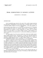
Figure 1: The 6-Vertex Model is defined on a n ×n grid. To each link in the network
we associate an arrow which can take two directions, the only constraint being that
at each site there are two arrows pointing in and two arrows pointing out (this leaves
6 possible vertex configurations). We are only interested in the configurations such

that the arrows at the top and at the bottom are pointing out and the arrows at the
left and the right are pointing in. Here we draw all states possibles for n = 3.
Thus, there are exactly 7 ASMs of size n = 3.
These matrices have been studied by Mills, Robbins and Rumsey since the early
1980s [14, 15, 21, 16]. It was then conjectured that A
n
, the number of ASMs of size
n, is given by:
A
n
=
n−1

j=0
(3j + 1)!
(n + j)!
= 1, 2, 7, 42, 429, . . . (2.1)
This was subsequently proved by Zeilberger in 1996 in an 84 page article [23].
A shorter proof was given by Kuperberg [12] in 1998. The latter is based on the
equivalence to the 6-V model, which we shall also use here.
2.2 6-Vertex model
Let us now turn to the 6-Vertex Model. The model consists in a square grid of size
n ×n in which each edge is given an orientation (an arrow), such that at each vertex
there are two arrows pointing in and two arrows pointing out. We use here some
very specific boundary conditions (Domain Wall Boundary Conditions, DWBC): all
arrows at the left and the right are pointing in and at the bottom and the top are
pointing out.
On figure 1 we draw all the possible configurations at n = 3. There are once again
7 configurations of size n = 3. Indeed, there is an easy bijection between ASMs and
6-V configurations with DWBC, which is described schematically on figure 2.

2.3 Totally Symmetric Self-Complementary Plane Partitions
We describe here Plane Partitions in two different ways, either pictorially or as arrays
of numbers.
the electronic journal of combinatorics 15 (2008), #R81 4
PSfrag replacements
0
0
0
0
1
-1
Figure 2: Rules to replace each vertex of a 6-V configuration with a 0 or ±1. Con-
versely, one can consistently build a 6-V configuration from an ASM starting from
the fixed arrows on the boundary, continuing arrows through the 0s and reversing
them through the ±1.
Pictorially, a plane partition is a stack of unit cubes pushed into a corner (gravity
pushing them to the corner) and drawn in isometric perspective, as examplified on
figure
3.
An equivalent way of describing these objects is to form the array of heights of
each stack of cubes. In this formulation the effect of “gravity” is that each number
in the array is less or equal than the numbers immediately above and to the left. For
example the plane partition on figure 3 may be translated into the array
75531
7433
6421
211
11
Plane partitions were first introduced by MacMahon in 1897. A problem of inter-
est is the enumeration of plane partitions that have some specific symmetries. The

Totally Symmetric and Self-Complementary Plane Partitions (TSSCPPs) are one of
these symmetry classes. In the pictorial representation, they are Plane Partitions
inside a 2n × 2n × 2n cube which are invariant under the following symmetries: all
permutations of the axes of the cube of size 2n×2n×2n; and taking the complement,
that is putting cubes where they are absent and vice versa, and flipping the resulting
set of cubes to form again a Plane Partition.
Alternatively, they can be described as 2n × 2n arrays of heights. In the n = 3
the electronic journal of combinatorics 15 (2008), #R81 5
Figure 3: We can see a plane partition (PP) as a stack of unit cubes pushed into a
corner.
case, we have, once again, 7 possible configurations:
666333 666433 666433 666543 666543 666553 666553
666333 666333 666433 665332 665432 655331 655431
666333 665332 664322 655331 654321 655331 654321
333000 433100 443200 533110 543210 533110 543210
333000 333000 332000 433100 432100 533110 532110
333000 332000 332000 321000 321000 311000 311000
(2.2)
and more generally we obtain A
n
for any n. In fact Zeilberger’s proof of the ASM con-
jecture amounts to showing (non-bijectively) that ASMs and TSSCPPs are equinu-
merous.
2.4 Non-Intersecting Lattice Paths
Another important class of objects is the Non-Intersecting Lattice Paths (NILPs).
These paths are defined in a lattice and connect a set of initial points to a set of final
points following certain rules (see Ref. [13, 7] for the general framework). The most
important feature of NILPs is that the various paths do not touch one another.
the electronic journal of combinatorics 15 (2008), #R81 6
0 0

00
0 1
0 0
0 00
2
0 0
0 0 0
1
1
0 0 0
0 1 0
2
0 0 0 0 0 0
1 1
1 2
1
0 00
1
0
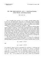
Figure 4: Reformulation of TSSCPPs as NCLPs, in the example of size n = 3. If
the origin is at the upper right corner, then at each point (0, −i), i ∈ {0, . . . , n −1},
begins a path which can only go upwards or to the right, and stops when it reaches
the diagonal (j, −j), in such a way that the numbers below/to the right of it are
exactly those less or equal to n − i.
In order to better understand the bijection between NILPs and TSSCPPs, it is
convenient to consider an intermediate class of objects: Non-Crossing Lattice Paths
(NCLPs), which are similar to NILPs except for the fact the paths are allowed to
share a common site, although they are still forbidden to cross each other.
We proceed with the description of the bijection between TSSCPPs and a class
of NCLPs. Each TSSCPP is defined by a subset of numbers of the arrays of (2.2), a

possible choice is the triangles at the bottom right:
0 1 2 1 2 1 2
00 00 00 10 10 11 11
000 000 000 000 000 000 000
It is easy to prove that this part of the array together with the symmetries which
characterize the TSSCPPs are enough to reconstruct the whole TSSCPP.
Then, we draw paths separating the different numbers appearing, as explained
on figure 4.
The bijection with the NILPs is easily achieved by shifting the paths (NCLPs)
according to the following rules:
• The i
th
path begins at (i, −i);
• The vertical steps are conserved and the horizontal steps (→) are replaced by
diagonal steps ().
An example (n = 3) is shown on figure 5.
Our last modification is the addition of one extra step to all paths. To the first
path we add a diagonal step, as for the other paths the choice is made such that
the difference between the final point of two consecutive paths is an odd number, as
examplified on figure 6.
the electronic journal of combinatorics 15 (2008), #R81 7
Figure 5: We transform our NCLPs into NILPs: the starting point is now shifted to
the right, and the horizontals steps become diagonal steps.
Figure 6: To each path we add one extra step in order that two final points consec-
utive differ by an odd number. The first extra step is diagonal.
3 The conjecture
Various conjectures have been made to connect ASMs and TSSCPPs. Building on
the already mentioned ASM conjecture by Mills and Robbins, which says that the
number of ASMs of size n is equal to the number of TSSCPPs of size 2n (and
which is now a theorem), there are conjectures about “refined” enumeration. Before

describing them we need some more definitions.
3.1 ASM generating function
Each ASM, as can be easily proven, has one and only one 1 on the first row and on
the last row. It is natural to classify ASMs according to their position. Therefore,
we count the ASMs of size n with the first 1 in the i
th
position and the last 1 in the
j
th
position:
˜
A
n,i,j
.
We build the corresponding generating function:
˜
A
n
(x, y) :=

i,j
˜
A
n,i,j
x
i−1
y
j−1
(3.1)
We define also A

n,i,j
, which counts the ASMs with the first 1 in the i
th
column
and the last 1 in the (n −j + 1)
st
column:
A
n,i,j
=
˜
A
n,i,n−j+1
(3.2)
And its generating function:
A
n
(x, y) :=

i,j
A
n,i,j
x
i−1
y
j−1
(3.3)
the electronic journal of combinatorics 15 (2008), #R81 8
Some trivial symmetries.
By reflecting the ASMs horizontally and vertically one gets:

A
n,i,j
= A
n,j,i
whereas by reflecting them only horizontally one gets:
A
n,i,j
= A
n,n−i+1,n−j+1
Obviously these symmetries are also valid for
˜
A
n,i,j
.
3.2 NILP generating function
First we recall the definition of the type of NILPs used in this article, of size n:
• The paths are defined on the square grid. Each step connects a site to a
neighbor and can be either vertical (up ↑) or diagonal (up right ).
• There are n starting points with coordinates (i, −i), i ∈ {0, 1, , n − 1}. The
endpoints are at (i, 0) (so that the length of the i
th
path is i).
• Paths do not touch each other.
It is convenient to add an extra step, as explained in section 2.4, defined uniquely
by the following:
• Two consecutive paths, after the extra step, differ by an odd number.
• The extra step for the first path (at (0, 0)) is diagonal.
Let α be a NILP, we define u
0
n

(α) as the number of vertical steps in the extra
step and u
1
n
(α) as the number of vertical step in the last step of each path (see
appendix A.1 for an extended definition).
The generating function is:
U
0,1
n
(x, y) :=

α
x
u
0
(α)
y
u
1
(α)
=

i,j
U
0,1
n,i,j
x
i
y

j
(3.4)
where U
0,1
n,i,j
is the number of NILPs of size n with i vertical extra steps and j vertical
last steps.
the electronic journal of combinatorics 15 (2008), #R81 9
3.3 The conjecture
We now present the conjecture, formulated by Mills, Robbins and Rumsey in a
slightly different language (see section A.2 for a detailed translation), whose proof is
the main focus of the present work:
Theorem. The number of ASMs of size n with the 1 of the first row in the (i + 1)
st
position and the 1 of last row in the (j + 1)
st
position is the same as the number
of NILPs (corresponding to TSSCPPs, and with the extra step) with i vertical extra
steps and j vertical steps in the last step. Equivalently,
˜
A
n
(x, y) = U
0,1
n
(x, y)
For example, at n = 3, using the ASMs given in section 2.1 and the TSSCPPs
given on figure 6, we compute:
˜
A

3
(x, y) =y
2
+ y + xy
2
+ x + xy + x
2
y + x
2
U
0,1
n
(x, y) =y
2
+ xy + x
2
+ xy
2
+ x
2
y + y + x
This is the doubly refined enumeration. Of course, by specializing one variable, one
recovers the simple refined enumeration, i.e. that the number of ASMs of size n with
the 1 of the first row in the i + 1 position is the same as the number of NILPs
(corresponding to the TSSCPPs and with the extra step) with i vertical extra steps:
A
n
(x) :=
˜
A

n
(x, 1) = U
0,1
n
(x, 1) := U
0
n
(x)
and by specializing two variables, that the number of ASMs of size n is the same as
the number of TSSCPPs of size 2n:
A
n
= A
n
(1) = U
0
n
(1)
4 The proof
4.1 ASM counting as the partition function of the 6-Vertex
model
In order to solve the ASM enumeration problem, it is convenient to generalize it
by considering weighted enumeration. This amounts to computing the partition
function of the 6-Vertex model, that is the summation over 6-V configurations with
DWBC such that to each vertex is given a statistical weight, as shown on figure 7,
the electronic journal of combinatorics 15 (2008), #R81 10
PSfrag replacements
a = q
−1/2
w − q

1/2
z
b = q
−1/2
z − q
1/2
w
c = (q
−1
− q)z
1/2
w
1/2
Figure 7: To each site configuration corresponds a statistical weight. These weights
depend on three parameters: w (resp. z) which characterizes the column (resp. row),
and a global parameter q which will be eventually specialized to a cubic root of unity.
depending on n horizontal spectral parameters (one for each row) {z
1
, z
2
, . . . , z
n
}, n
vertical spectral parameters {z
n+1
, z
n+2
, . . . , z
2n
} and one global parameter q. This

computation was performed by Izergin [
8], using recursion relations written by Ko-
repin [11], and the result is a n ×n determinant (IK determinant). It is a symmetric
function of the set {z
1
, . . . z
n
} and of the set of {z
n+1
, . . . , z
2n
}. Much later, it was ob-
served by Stroganov [22] and Okada [17] that when q = e
2πi/3
, the partition function
is totally symmetric, i.e. in the full set {z
1
, . . . , z
2n
}.
More precisely, if we denote by
˜
Z
n
the partition function, and
Z
n
= (−1)
n(n−1)/2
(q

−1
− q)
−n
2n

i=1
z
−1/2
i
˜
Z
n
then Z
n
was identified at q = e
2πi/3
with the Schur function corresponding to the
Young diagram Y
n
with two rows of length n −1, two rows of length n −2, . . . , two
rows of length 2 and two rows of length 1:
Z
n
(z
1
, . . . z
2n
) = s
Y
n

(z
1
, . . . , z
2n
) =
det[z
2n−j+d
j
i
]
det[z
2n−j
i
]
(4.1)
where d
j
is the sequence {n −1, n−1, n −2, n −2, . . . , 2, 2, 1, 1, 0, 0}. This formula is
proved in appendix B, though its explicit form will not be needed in what follows.
With this method we recover the unweighted enumeration by setting all z
i
= 1:
3
−n(n−1)/2
Z
n
(1, . . . , 1) = A
n
(4.2)
where we recall that A

n
is the number of ASMs of size n (as explained in 2.1).
The case of interest to us is when all z
i
= 1 except z
1
and z
2n
:
z
1
=
1 + qt
q + t
z
2n
=
1 + qu
q + u
the electronic journal of combinatorics 15 (2008), #R81 11
Using the fact that Z
n
(z
1
, . . . , z
2n
) is a symmetric function of its arguments (see
appendix B), we have
Z
n

(z
1
=
1 + qt
q + t
, 1, . . . , 1, z
2n
=
1 + qu
q + u
)
= Z
n
(z
1
=
1 + qt
q + t
, 1, . . . , 1, z
n
=
1 + qu
q + u
, 1, . . . , 1)
The corresponding weights take the form
a
x
= q
−
1

2
− q
1
2

1 + qx
q + x

=
q
1
2
x
q + x
(q
−1
− q)
b
x
= q
−
1
2

1 + qx
q + x

− q
1
2

=
q
1
2
q + x
(q
−1
− q)
c
x
= (q
−1
− q)

1 + qx
q + x
The partition function
˜
Z
n
becomes
˜
Z
n
= (−i
√
3)
n
2
−2n


j,k
a
j−1
t
b
n−j
t
c
t
a
k−1
u
b
n−k
u
c
u
A
n,j,k
= (−i
√
3)
n
2

1 + qt
q + t

1 + qu

q + u

1
q + t

n−1

1
q + u

n−1
q
n−1

j,k
t
j−1
u
k−1
A
n,j,k
where A
n,j,k
is the number of ASMs of size n such that the only 1 in the first row is
in column j and the only 1 in the last row is in column n −k + 1.
The normalization factor is equal to: (−1)
n(n−1)/2
(−i
√
3)

n

1+qt
q+t

1+qu
q+u
, so we
can finally compute
(q
2
(q + t)(q + u))
n−1
3
n(n−1)/2
Z
n
=

j,k
t
j−1
u
k−1
A
n,j,k
= A
n
(t, u) (4.3)
Note that if one uses instead z

2n
=
q+u
1+qu
, one gets the same formula, but with
one index reversed
(q
2
(q + t)(1 + qu))
n−1
3
n(n−1)/2
Z
n
=
˜
A
n
(t, u) (4.4)
the electronic journal of combinatorics 15 (2008), #R81 12
4.2 Integral formula for refined ASM counting
The traditional expression for the partition function of the 6-V model is the already
mentioned IK formula. We shall not use it here. We shall only need the following
facts (true at q = e
2πi/3
):
• Z
1
= 1.
• Z

n
(z
1
, . . . , z
2n
) is a polynomial of degree n −1 in each variable.
• The Z
n
satisfy the recursion relation for all i, j = 1, . . . , 2n
Z
n
(z
1
, . . . , z
j
= q
2
z
i
, . . . , z
2n
) =

k=i,j
(qz
i
− z
k
)Z
n−1

(z
1
, . . . , ˆz
i
, . . . , ˆz
j
, . . . , z
2n
)
(4.5)
We recall how to prove them in appendix B for the sake of completeness.
Furthermore, we need the following lemma
Lemma 1. A polynomial P of degree n−1 in each variable z
1
, . . . , z
2n
which satisfies
the “wheel condition”
P (. . . , z
i
= z, . . . , z
j
= q
2
z, . . . , z
k
= q
4
z, . . .) = 0 for all i < j < k
is entirely determined by its c

n
:= (2n)!/n!/(n + 1)! values at the following special-
izations: (q

1
, . . . , q

2n
) for all possible choices of {
i
= ±1} such that

2n
i=1

i
= 0
and

j
i=1

i
≤ 0 for all j ≤ 2n.
This lemma is proved in appendix C.
The strategy is now to introduce a certain integral representation of the partition
function of the 6-V model with DWBC, say Z

n
Z


n
:= (−1)
(
n
2
)
2n

i<j
(qz
i
− q
−1
z
j
)

. . .

n

l
dw
l
2πi
(qz
2l−1
− q
−1

w
l
)

l<m
(w
m
− w
l
)(qw
l
− q
−1
w
m
)

i≤2l−1
(w
l
− z
i
)

i≥2l−1
(qw
l
− q
−1
z

i
)
(4.6)
where the integration contours surround counterclockwise the z
i
(but not the q
−2
z
i
),
and to show that Z
n
and Z

n
are both polynomials of degree n − 1 in each variable
which satisfy the “wheel condition” and coincide at the c
n
specializations of lemma 1.
the electronic journal of combinatorics 15 (2008), #R81 13
Let us first check that Z
n
satisfies the wheel condition. This is a direct conse-
quence of Eq. (4.5) in which one sets z
k
= q
4
z
i
. It is equally straightforward to

calculate Z
n
at the c
n
points of the lemma. The computation goes inductively using
Eq. (4.5) and it is left to the reader to check that
Z
n
(q

1
, . . . , q

2n
) = 3
(
n
2
)
We now show that Z

n
also satisfies the hypotheses of the lemma. We proceed in
steps.
Z

n
is a polynomial of degree n − 1 in each variable.
By applying the residue formula to Eq. (4.6) we obtain
Z


n
= (−1)
(
n
2
)

K=(k
1
, ,k
n
)
k
l
=k
m
if l=m
k
l
≤2l−1
(−1)
s(K)

l<m
(qz
k
l
− q
−1

z
k
m
)
×

i<j
i/∈K or (i=k
l
and j<2l−1)
(qz
i
− q
−1
z
j
)

2i−1=k
i
(qz
2i−1
− q
−1
z
k
i
)

i≤2j−1

i/∈K or i>k
j
(z
k
j
− z
i
)
(4.7)
where (−1)
s(K)
is the sign of the permutation that orders the k
i
. It is enough to
prove that lim
z
k
j
→z
i
Z

n
exists; the verification is a tedious but easy calculation (see
[6] for a similar check).
We can now consider the leading term in each variable z
i
in the summation of
Eq. (4.7), depending on whether i ∈ K or not; in both cases we find a degree n −1.
Z


n
satisfies the wheel condition.
Using the formula (4.7), we can verify that Z

n
is zero at z
k
= q
2
z
j
= q
4
z
i
for all
k > j > i: In fact, the term

s<r and s/∈K
(qz
s
−q
−1
z
r
) implies that i and j ∈ K. As a
consequence of the term

l<m

(qz
k
l
−q
−1
z
k
m
), we must have i = k
m
and j = k
l
with
l < m, but, in this case, j ≤ 2l − 1 < 2m − 1 proving that Z

n
satisfies the “wheel
condition”.
the electronic journal of combinatorics 15 (2008), #R81 14
Recursion relation.
We show that Z

n
, at q = e
2πi/3
, satisfies a weaker form of recursion relation (4.5).
Let j be an integer between 1 and 2n − 1 and evaluate Z

n
at z

j+1
= q
2
z
j
. We will
perform the calculation for j even.
If we look at formula (4.7) it is straightforward that all terms are zero except for
j = k
m
and j + 1 ≥ 2m − 1, i.e. j = k
m
= 2m − 2. Using the fact that z
j+1
= q
2
z
j
,
we can derive
Z

n|z
j+1
=q
2
z
j
=


i<j
(qz
i
− q
−1
z
j
)(qz
i
− qz
j
)

k>j+1
(qz
j
− q
−1
z
k
)(z
j
− q
−1
z
k
)(−1)
(
n
2

)
×

i<k=j,j+1
(qz
i
− q
−1
z
k
)

. . .


l
dw
l
2πi

l=m
(qz
2l−1
− q
−1
w
l
)
×


l<p=m
(w
p
− w
l
)(qw
l
− q
−1
w
p
)(z
j
− q
−1
z
j
)

l=m

i≤2l−1
i=j,j+1
(w
l
− z
i
)

i≥2l−1

i=j,j+1
(qw
l
− q
−1
z
i
)
×

n>m
(w
n
− z
j
)(qz
j
− q
−1
w
n
)
(w
n
− z
j
)(w
n
− q
2

z
j
)

l<m
(z
j
− w
l
)(qw
l
− q
−1
z
j
)
(qw
l
− q
−1
z
j
)(qw
l
− qz
j
)
×
1
(z

j
− q
2
z
j
)

i<j
(z
j
− z
i
)

k>j+1
(qz
j
− q
−1
z
k
)
After multiple cancellations we get:
Z

n
(. . . , z
j
, z
j+1

= q
2
z
j
, . . .) =

i=j,j+1
(qz
j
− z
i
)Z

n−1
(z
1
, . . . , z
j−1
, z
j+2
, . . . , z
2n
) (4.8)
The formula actually holds for both parities of j; the proof for j odd is similar.
Calculating Z

n
at the c
n
points.

Using the formula above, we can easily calculate Z

n
at the c
n
points of the lemma.
One can always choose two consecutive variables which are (q
−1
, q) and apply the
recursion relation above:
Z

n
(. . . , z
j
= q
−1
, z
j+1
= q
2
z
j
= q, . . .) =

i=j,j+1
(1 −z
i
)Z


n−1
= (1 − q)
n−1
(1 − q
−1
)
n−1
Z

n−1
The second equality uses the fact that there is the same number of 
i
= 1 and

i
= −1. Since we have Z

1
= 1, we obtain:
Z

n
= 3
(
n
2
)
the electronic journal of combinatorics 15 (2008), #R81 15
We finally conclude, by applying lemma 1, that
Z

n
= Z

n
Starting from our new integral formula for the partition function of the 6-Vertex
model (4.6), we are now in a position to calculate
(q
2
(q + x)(1 + qy))
n−1
(q − q
−1
)
n(n−1)
Z
n
(
1 + qx
q + x
, 1, . . . , 1,
q + y
1 + qy
)
After some tedious computations and using new variables
u
i
=
w
i
− 1

qw
i
− q
−1
we obtain:
(y + x − yx)

. . .

n

l
du
l
2πi
1
u
2l−2
l

l<m
(u
m
− u
l
)(1 + u
m
+ u
m
u

l
)
(1 + u
l
− x)(1 + u
l
(1 −y))
n

j=2
(1 + u
j
)
where the integral contours surround counterclockwise u
i
= 0 and u
i
= x − 1 (and
not 1/(y − 1)).
To simplify our calculation we integrate on u
1
:
˜
A
n
(x, y) =

. . .

n


l=2
du
l
2πi
(1 + u
l
)(1 + xu
l
)
u
2l−2
l
(1 + u
l
(1 −y))
n

l<m
(u
m
− u
l
)(1 + u
m
+ u
m
u
l
) (4.9)

where the contours surround the remaining poles at u
i
= 0 only.
4.3 Integral formula for refined NILP counting
We will derive a contour integral formula for the generating polynomial N

10
(t
0
, t
1
, . . .,
t
n−1
) of our NILPs with a weight t
i
per vertical step in the i
th
slice (between y = 1−i
and y = −i). We use the Lindstr¨om–Gessel–Viennot formula [13, 7] (see also the
third chapter of [2]):
N

10
(t
0
, t
1
, . . . , t
n−1

) =

1=r
1
< <r
n−1
r
i
≤2i+1
r
i+1
−r
i
odd
det[P
i,r
j
] (4.10)
the electronic journal of combinatorics 15 (2008), #R81 16
where P
i,r
is the weighted sum over all possible lattice paths from (i, −i) to (r +1, 1).
Such paths counts with r − i + 1 diagonal steps and 2i − r vertical ones, hence:
P
i,r
=

0≤i
1
< <i

2i−r
≤i
2i−r

l=1
t
i
l
=
i

k=0
(1 + t
k
u)|
u
2i−r
(4.11)
where the subscript u
2i−r
stands for the coefficient of the corresponding power of u
in the polynomial.
We can reintroduce the path beginning at (0, 0) and rewrite the equation as a
contour integral:
N

10
(t
0
, t

1
, . . . , t
n−1
) =

. . .

n

i=1
du
i
2πiu
2i−1
i
i−1

k=0
(1 + t
k
u
i
)

0=r
0
<r
1
< <r
n−1

r
i+1
−r
i
odd
det[u
r
j−1
i
]
where the paths of integrations are small counterclockwise circles around zero.
The last sum can be evaluated as a standard result for the sum over all Schur
functions corresponding to even partitions (see exercise 4.3.9 in [2]):

0=r
0
<r
1
< <r
n−1
r
i+1
−r
i
odd
det[u
r
j−1
i
] =


j>i
(u
j
− u
i
)

j≥i
(1 − u
j
u
i
)
(4.12)
where we have relaxed the condition r
0
= 0 into r
0
≥ 0 and even, since this does not
affect the integral.
The integral can thus be transformed as follows:
N

10
(t
0
, t
1
, . . . , t

n−1
) =

. . .

n

i=1
du
i
2πiu
2i−1
i
1
1 − u
2
i
i−1

k=0
(1 + t
k
u
i
)

j>i
u
j
− u

i
1 −u
j
u
i
(4.13)
We are mainly interested in the case where t
0
= t, t
1
= s and all the others t
i
equal 1. In this case, we rewrite the equation:
N

10
(t, s, 1, . . . , 1) := U
0,1
n
(t, s)
=

. . .

n

i=1
du
i
2πiu

2i−1
i
1
1 − u
2
i
(1 + tu
i
)(1 + su
i
)
ˆ
1
(1 + u
i
)
i−2
ˆ
1

j>i
u
j
− u
i
1 − u
j
u
i
(4.14)

where
ˆ
1 means that we exclude the term corresponding to u
1
.
the electronic journal of combinatorics 15 (2008), #R81 17
4.4 Equality of integral formulae
At this point, we have two integral expressions, A
n
(x, y) (in equation (4.9)) and
U
0,1
n
(x, y) (in equation (4.14)) and we want to prove that they are the same. The
first step is to integrate over u
1
the expression (4.14):
U
0,1
n
(x, y) =

. . .

n

i=2
du
i
2πiu

2i−2
i
(1 + xu
i
)(1 + yu
i
)(1 + u
i
)
i−2

i<j
(u
j
− u
i
)

i≤j
(1 −u
j
u
i
)
(4.15)
At this stage we use the following identity:

. . .



i
du
i
2πi
ϕ(u)
u
2i
i

i<j
(u
j
− u
i
)(1 + τ u
j
+ u
i
u
j
)
=

. . .


i
du
i
2πi

ϕ(u)
(1 + τ u
i
)
i−1
u
2i
i

i<j
(u
j
− u
i
)

i≤j
(1 −u
i
u
j
)
(4.16)
for any ϕ(u) completely symmetric in (u
1
, u
2
, . . . , u
n
) and without poles in a neigh-

borhood of zero. This was conjectured in [6] and proved in [24]. We present in
appendix D an independent proof of a stronger formula that implies Eq. (4.16).
If we shift the indexes (i − 1) → i, consider τ = 1 and set ϕ(u) =

n−1
i=1
(1 +
xu
i
)(1 + yu
i
) we can apply the equality:
U
0,1
n
(x, y) =

. . .

n

i=2
du
i
2πiu
2i−2
i
(1+xu
i
)(1+yu

i
)

i<j
(u
j
−u
i
)(1+u
j
+u
j
u
i
) (4.17)
Notice that the two integrals are the same, except for the pieces
(1+u
l
)
(1+u
l
(1−y))
versus
1 + yu
l
. Unsurprisingly, we find that is possible to write both integrals as special
cases of the same integral:
I
n
(x, y) =


. . .

n−1

l=1
du
l
2πi
(1 + u
l
+ a
l
u
2
l
)(1 + xu
l
)
u
2l
l
(1 + u
l
(1 −y))
n−1

l<m
(u
m

− u
l
)(1 + u
m
+ u
m
u
l
)
(4.18)
which takes the value of
˜
A
n
(x, y) if a
l
= 0 for all l and takes the value of U
0,1
(x, y)
if a
l
= y(1 − y) for all l.
More surprising is the fact that I
n
does not depend on the a
i
. We shall show by
induction on i that I
n
is independent of a

i
, noting that it is a polynomial in a
i
of
degree at most 1.
the electronic journal of combinatorics 15 (2008), #R81 18
Let us first differentiate I
n
with respect to a
1
:
d
da
1
I
n
(x, y) =

du
1
2πi
(1 + xu
1
)
(1 + u
1
(1 − y))
×

. . .


n−1

l=2
du
l
2πi
(1 + u
l
+ a
l
u
2
l
)(1 + xu
l
)
u
2l
l
(1 + u
l
(1 −y))
n−1

m<l
(u
l
− u
m

)(1 + u
l
+ u
m
u
l
)
but, this integral has no poles at u
1
so it vanishes.
Let us now assume by induction hypothesis that I
n
does not depend on the first
(i −1) a
j
, and prove that the expression (4.18) does not depend on a
i
either. As the
integral does not depend on a
j
for all j < i we can set all a
j
= 0 (for j < i).
If we differentiate now with respect to a
i
and look at what happens in the inte-
gration up to u
i
. We find an expression of the type:
J

i
=

du
i
2πiu
2i−2
i

···

i−1

j=1
du
j
2πi
1 + u
j
u
2j
j
Θ
i
A
i
(4.19)
where A
i
is some anti-symmetric function in the u

j
for all j ≤ i without any poles
in the integration domain, and Θ
i
=

j<i
(1 + u
i
+ u
j
u
i
).
To prove that this integral is always zero we shall proceed once again by induction.
The first one, J
1
, is zero because it has no poles:
J
1
=

du
1
2πi
A
1
(x
1
) = 0 (4.20)

Let J
i−1
= 0. All the poles are at 0, the A
i
is anti-symmetric between u
i
and
u
i−1
, so we can take advantage of the fact that the u
i
appears with the same degree
as u
i−1
in the denominator to erase all the symmetric terms in the expression (1 +
u
i−1
)(1 + u
i
+ u
i−1
u
1
) and get u
i
u
2
i−1
:
J

i
=

du
i
2πiu
2i−3
i

du
i−1
2πiu
2i−4
i−1

. . .

i−2

j=1
du
j
2πi
1 + u
j
u
2j
j
ˆ
Θ

i
A
i
(4.21)
where the hat in
ˆ
Θ
i
means that the term (1 + u
i
+ u
i−1
u
i
) is skipped
1
. The integral
does not have yet the desired form, i.e. J
i−1
, it is missing the term (1 + u
i
+ u
i−1
u
i
),
1
Note that
ˆ
Θ

i
is symmetric between u
i−1
and u
i
.
the electronic journal of combinatorics 15 (2008), #R81 19
so we add and subtract it:
J
i
=

. . .

du
i
2πiu
2i−3
i
du
i−1
2πiu
2i−4
i−1
i−2

j=1
du
j
2πi

1 + u
j
u
2j
j
(1 + u
i
+ u
i
u
i−1
− u
i
− u
i
u
i−1
)
ˆ
Θ
i
A
i
=

. . .

du
i
2πiu

2i−3
i
du
i−1
2πiu
2i−4
i−1
i−2

j=1
du
j
2πi
1 + u
j
u
2j
j
Θ
i
A
i
−

. . .

du
i
2πiu
2i−4

i
du
i−1
2πiu
2i−4
i−1
i−2

j=1
du
j
2πi
1 + u
j
u
2j
j
(1 + u
i−1
)
ˆ
Θ
i
A
i
The first term is already in the form of J
i−1
. The second term is almost symmetric
between u
i

and u
i−1
, using the same method as in (4.21) we can transform −(1+u
i−1
)
to 1 + u
i
+ u
i
u
i−1
; in this way, we recover the symmetry needed so that we can write
J
i
as an integral in u
i
of some function multiplied by J
i−1
, which is zero. As a
consequence J
i
is also zero for all i, i.e. I
n
(x, y) does not depend on any a
i
. We
conclude that
˜
A
n

(x, y) = U
0,1
n
(x, y)
A Formulating the conjecture directly in terms of
TSSCPPs
We have used the NILP formulation throughout this paper (in particular, to prove the
main theorem), whereas Mills, Rumsey and Robbins use the language of TSSCPPs.
In A.1 we first describe the theorem in a more general form, and then prove that we
can reduce it to the one presented in 3.3. We then reformulate in A.2 our theorem
in the language of [16, 20].
A.1 Extending the theorem
Let A
n
(x, y) and
˜
A
n
(x, y) be the same as defined in 3.1. We use the same NILPs
with the extra-step as in 3.2.
We now introduce a function u
k
n
(α), where α is a NILP, which counts the number
of vertical steps in the extra-step if k = 0; otherwise it counts the number of vertical
steps in the max{1, t − k + 1}-th step of the path starting at (t, −t), as shown on
figure 8.
the electronic journal of combinatorics 15 (2008), #R81 20
PSfrag replacements
u

0
6
u
3
6
Figure 8: Let α be the NILP represented here. In order to calculate u
0
6
(α) and u
3
6
(α)
we highlight the extra-steps and the max{1, t − 3 + 1}-th step of the path starting
at (t, −t). Here we have u
0
6
(α) = 2 and u
3
6
(α) = 4.
We can next define the function U
i
n
(x):
U
i
n
(x) :=

k

U
i
n,k
x
k
:=

α
x
u
i
n
(α)
(A.1)
and more complex functions U
i,j
n
(x, y):
U
i,j
n
(x, y) :=

k
U
i,j
n,k,l
x
k
y

l
:=

α
x
u
i
n
(α)
y
u
j
n
(α)
(A.2)
We could generalize these even more, introducing more indices, but this is general
enough for our purposes. With these new functions we can rewrite our theorem:
Theorem.
˜
A
n
(x, y) = U
0,j
n
(x, y) (A.3)
A
n
(x, y) = U
1,i
n

(x, y) (A.4)
where j = 1, 2 . . . and i = 2, 3 . . If we choose U
0,1
n
we have the theorem as stated
before.
On order to reduce this to our previous result, it is enough to prove that U
0,i
n
does not depend in i and that U
0,i
n,k,j
= U
1,i
n,n−k−1,j
(for i ≥ 2).
i independence of U
0,i
n
.
For the first equality we introduce a function g as explained on figure
9. This function
interchanges the number of vertical steps in two consecutive rows leaving invariant
all the other rows. This function has the important property g ◦ g = Id. So, it is
straightforward from this that U
0,i
n
= U
0,i+1
n

, with i greater than 0.
the electronic journal of combinatorics 15 (2008), #R81 21
Figure 9: We can group the double steps in islands, such that all the starting points
(of the double steps) are consecutive. These doubles steps are, necessarily, ordered
in r double vertical steps, s vertical-diagonal steps, t diagonal-vertical steps and u
double diagonal steps. Our function g interchanges s with t at each island, so that
we interchange the number of vertical steps between the two rows.
Figure 10: In order to satisfy the extra-step rules we can only build two type of
islands, one made of r double vertical steps and s double diagonal steps, and the
other type made of t vertical-diagonal steps and u diagonal-vertical steps. Our
function h interchange simply r with s. It is important to note that the first path is
always invariant under h (it is always of the type vertical-diagonal or the inverse).
U
0,i
n,k,j
= U
1,i
n,n−k−1,j
for i > 1.
The proof follows the same structure as the former. We construct again a function
h such that h ◦h = Id, which interchanges the number of vertical steps at the extra-
step with the number of diagonal steps at the last step (before the extra-step). This
function is obviously a bijection and it leaves invariant all the rows except the last
one and the extra one because it is applied at the top of the diagrams as can be seen
on figure 10. An important remark is that the first path is always invariant under
h because it is of the type vertical-diagonal or diagonal-vertical. This proves our
equality.
In conclusion, all these variations ((A.3) and (A.4)) are truly the same, and we
can concentrate on only one version.
A.2 The conjecture in terms of TSSCPPs

Mills, Robbins and Rumsey conjectured this theorem by means of TSSCPPs, not
NILPs, but behind the different formulations lies the same result. To show that, we
describe some of the content of [16] and explain the equivalence.
Recall that TSSCPPs can be represented as 2n × 2n matrices a, as in Eq. (2.2).
In [16] is introduced a quantity which we shall denote by u
k
n
(a), and which depends
the electronic journal of combinatorics 15 (2008), #R81 22
0 0
00
0 1
0 0
0 00
2
0 0
0 0 0
1
1
0 0 0
0 1 0
2
0 0 0 0 0 0
1 1
1 2
1
0 00
1
0
Figure 11: We can see on this figure what the function u

2
3
counts. The signs minus
represents the part: a
t,t−k
− a
t,t−k+1
, so they count the vertical steps, and the little
circles represents #{a
t,n+1
| a
t,n+1
< 2n − t}. If we stretch our diagrams to obtain
the NILPs we recover our definition of u
k
n
.
on the upper-left n × n submatrix of a:
u
k
n
(a) =
n−k+1

t=1
(a
t,t+k−1
− a
t,t+k
) +

n

t=n−k+2
#{a
t,n
| a
t,n
> 2n − t + 1} (A.5)
where # means cardinality, and where conventionally, a
t,n+1
:= 2n − t + 1 in this
equation. Also defined is the function:
U
i, k
n
(x, . . . , z) =

a
x
u
i
n
(a)
. . . z
u
k
n
(a)
for all i, . . . , k ∈ {1, . . . , n + 1} (A.6)
We claim that these are our functions u and U defined above. To make the con-

nection, reexpress this function in terms of the lower-right n × n submatrix of a:
u
k
n
(a) =
2n

t=n+k
(a
t,t−k
− a
t,t−k+1
) +
n+k−1

t=n+1
#{a
t,n+1
| a
t,n+1
< 2n − t} (A.7)
where we replace a
t,n
with 2n−t. What this function counts is described on figure 11.
Finally, if we shift the diagrams to obtain NILPs we recover our functions U
k
n
as
expected.
As a final remark, in the article [20] three functions are defined: f

1
, f
2
and f
3
and the conjecture is stated with any two of them. In fact, f
1
is connected with the
u
0
n
, f
2
with the u
1
n
and f
3
with u
n
n
, as can be seen using the same procedure.
B Properties of the 6-Vertex model partition
function
Consider, as in section 4.1, the 6-Vertex model with Domain Wall Boundary Condi-
tions. Let
˜
Z
n
be its partition function (with Boltzmann weights given by Fig. 7), and

Z
n
to be
˜
Z
n
divided by the normalization factor (−1)
n(n−1)/2
(q
−1
− q)
n

2n
i=1
z
1/2
i
.
the electronic journal of combinatorics 15 (2008), #R81 23
PSfrag replacements
z
1
z
1
z
2
z
2
w

w
Figure 12: Yang–Baxter equation. Summation over arrows of the internal edges is
implied, while the external arrows are fixed and the equality holds for any choice of
them.
The model thus defined satisfies the following essential property (Yang–Baxter
equation) shown on Fig.
12. The vertex with diagonal edges is assigned weights (the
so-called R matrix) which are those of Fig. 7 in which we have rotated the picture
45 degrees clockwise, and with parameters z
1
, q
1/2
z
2
. parameter. In fact here we
do not need the explicit expression of the R matrix, only that it is invariant by
reversal of all arrows and that it satisfies the ice rule i.e. there are as many outgoing
arrows as incoming arrows. Since the Yang–Baxter equation is invariant by change of
normalization of R, we can divide all weights by b in such a way that R
↑↑
↑↑
= R
↓↓
↓↓
= 1,
with obvious notations.
B.1 Korepin recursion relation
In this paragraph, q is kept arbitrary. We shall now list the following four proper-
ties which determine entirely Z
n

and only sketch their proof (since they have been
reproved many times since their original appearance [11], see for example [12, 10])
• Z
1
= 1.
This is by definition.
• Z
n
is a symmetric function of the variables {z
1
, . . . , z
n
} and {z
n+1
, . . . , z
2n
}.
It is sufficient to prove that exchange of z
i
and z
i+1
(for 1 ≤ i < n) leaves
the partition function unchanged. This can be obtained by repeated use of the
Yang–Baxter property. Multiplying the partition function by R(z
i+1
/z
i
) and
the electronic journal of combinatorics 15 (2008), #R81 24
noting that it is unchanged, we find

˜
Z
n
(. . . , z
i
, z
i+1
, . . .) =
PSfrag replacements
z
i
z
i+1
=
PSfrag replacements
z
i
z
i+1
=
PSfrag replacements
z
i
z
i+1
= ··· =
PSfrag replacements
z
i
z

i+1
=
PSfrag replacements
z
i
z
i+1
=
˜
Z
n
(. . . , z
i+1
, z
i
, . . .)
and similarly for the {z
n+1
, . . . , z
2n
}.
• Z
n
(z
1
, . . . , z
2n
) is a polynomial of degree (at most) n −1 in each variable.
Let us choose one configuration. Then the only weights which depend on z
i

are
the n weights on row i. Since the outgoing arrows are in opposite directions,
the number of vertices of type c on this row is odd, and in particular is at least
1. Power counting then shows that the contribution to the partition function
of any configuration is of the form z
1/2
i
times a polynomial of z
i
of degree at
most n − 1. Summing over all configurations and removing z
1/2
i
by definition
of Z
n
, we obtain the desired property.
• The Z
n
obey the following recursion relation:
Z
n
(z
1
, . . . , z
n
; z
n+1
= q
−1

z
1
, . . . , z
2n
)
= q
−n+1
n

j=2
(z
1
− q
2
z
j
)
2n

j=n+2
(z
1
− q
−1
z
j
)Z
n−1
(z
2

, . . . , z
n
; z
n+2
, . . . , z
2n
) (B.1)
Since z
n+1
= q
−1
z
1
implies a(z
n+1
, z
1
) = 0, by inspection all configurations
with non-zero weights are of the form shown on Fig.
13. This produces the
following identity for unnormalized partition functions
˜
Z
n
(z
1
, . . . , z
n
; z
n+1

= q
−1
z
1
, . . . , z
2n
) = (q
−1
− q)z
1
q
−1/2
×
n

j=2
(q
−3/2
z
1
− q
1/2
z
j
)
2n

j=n+2
(q
−1/2

z
j
− q
1/2
z
1
)
˜
Z
n−1
(z
2
, . . . , z
n
; z
n+2
, . . . , z
2n
)
the electronic journal of combinatorics 15 (2008), #R81 25