Báo cáo toán học: "Compression of root systems and the E-sequence" pptx
Bạn đang xem bản rút gọn của tài liệu. Xem và tải ngay bản đầy đủ của tài liệu tại đây (218.8 KB, 21 trang )
Compression of root systems and the E-sequence
Kevin Purbhoo
∗
Submitted: Aug 25, 2007; Accepted: Apr 22, 2008; Published: Sep 15, 2008
Mathematics Subject Classification: 17B20
Abstract
We examine certain maps from root systems to vector spaces over finite fields.
By choosing appropriate bases, the images of these maps can turn out to have nice
combinatorial properties, which reflect the structure of the underlying root system.
The main examples are E
6
and E
7
.
1 Introduction
The primary goal of this paper is to provide a convenient way of visualising the root
systems E
6
and E
7
. There are two important relations on a root system that one might
wish to have a good understanding of: the poset structure, in which α > β if α − β is
a sum of positive roots, and the orthogonality structure, in which α ∼ β if α and β are
orthogonal roots.
In our paper on cominuscule Schubert calculus, with Frank Sottile [8], we found that
our examples required a good simultaneous understanding both these structures. This is
easy enough to acquire for the root systems corresponding to the classical Lie groups. In
A
n
, for example, one can visualise the positive roots as the entries of an strictly upper
triangular (n + 1) × (n + 1) matrix, where the ij position represents the root x
i
− x
j
.
Then α ≥ β if and only if α is weakly right and weakly above β. Orthogonality is also
straightforward in this picture: α and β are non-orthogonal if there is some i such that
crossing out the i
th
row and the i
th
column succeeds in crossing out both α and β. Figure 1
shows the roots orthogonal to x
3
− x
5
in A
5
.
In type E, it is less obvious how to draw such a concrete picture. Separately the
two structures have been well studied in the contexts of minuscule posets [7, 9, 11], and
strongly regular graphs (see e.g. [1, 3, 4]). However, once one draws the Hasse diagram of
the posets, the orthogonality structure suddenly becomes mysterious. Of course, one can
always calculate which pairs of roots are orthogonal, but we would prefer a picture which
allows us to do it instantly. Thus the main thrust of this paper is to get to Figures 4 and 6,
∗
Department of Combinatorics and Optimization, University of Waterloo, Waterloo, ON, N2L 3G1,
Canada;
the electronic journal of combinatorics 15 (2008), #R115 1
46
3534
26
36
15 1612 13 14
23 24 25
45
56
Figure 1: Orthogonality and partial order in type A.
which illustrate how one can simultaneously visualise E
7
and E
6
posets and orthogonality
structures, at least restricted to certain strata of the root system. The restriction of these
structures to the strata is exactly what is needed for the type E examples in [8]. With a
little more work, one can use these figures to recover the partial order and orthogonality
structures for the complete root system.
To reach these diagrams, we begin by considering certain maps from a root system
to (Z/p)
m
, which are injective (or 2:1 if p = 2). In Section 2, we make some general
observations about these maps. Then, in Section 3 we give examples for E
6
and E
7
which
are particularly nice. In these cases, we show that properties of the underlying root system
are reflected in simple combinatorial structures on the target space, which is what allows
us to produce diagrams in question. As the E
7
example is richer, we will discuss it before
the E
6
example. Finally, in Section 4, we discuss how the partial order structures on each
of the strata are related by order ideals. This relationship plays an essential role in [8],
and is useful for understanding the structure of the E
8
root system.
The idea of relating the E
6
and E
7
root systems to (Z/p)
m
has appeared elsewhere.
For example, Harris [5] uses such an identification to describe the Galois group of the 27
lines on the cubic surface, one of the del Pezzo surfaces. The connection between del Pezzo
surfaces and the exceptional Lie groups has been well established; we refer the reader to
[6]. One can also see such a relationship reflected in the well known identification of Weyl
groups (see e.g. [2]):
W (E
6
)
∼
=
SO(5; Z/3)
∼
=
O
−
(6; Z/2),
W (E
7
)
∼
=
Z/2 × Sp(6; Z/2).
These facts follow from the identifications outlined in this paper, and presumably have
been proved in similar ways before. (To see that W (E
7
) identification is a direct product
rather than a semidirect product, one needs the additional fact that the long word w
0
∈
W (E
7
) is central.)
The author is grateful to Hugh Thomas and Richard Green for their comments on this
paper. This work was partially supported by NSERC.
the electronic journal of combinatorics 15 (2008), #R115 2
2 Compression of root systems
2.1 Simply laced root systems
Let ∆ ⊂ R
n
be a simply laced root system. Let ·, · denote the inner product on R
n
,
for which we have β, β = 2 for all β ∈ ∆. We assume that ∆ has full rank in R
n
. Let
Λ = Z∆ denote the lattice in R
n
generated by ∆.
Throughout, we will make use of the fact that if α and β are roots in a simply laced
root system ∆, then α + β ∈ ∆ if and only if α, β = −1. Similarly, we have α − β ∈ ∆
if and only if α, β = 1.
Choose a basis of simple roots α
1
, . . . , α
n
∈ ∆, for Λ. Let ∆
+
denote the positive roots
with respect to this basis, and ∆
−
denote the negative roots. Recall that ∆
+
is a partially
ordered set, with β > β
iff β − β
is a sum of positive roots. Roots β and β
are always
comparable in the partial ordering when β, β
> 0, though the converse is not true.
For each β ∈ Λ, we define β
i
to be the coefficient of α
i
, when β is expressed in the
basis of the simple roots: β =
n
i=1
β
i
α
i
.
Let Dyn denote the Dynkin diagram of ∆. As ∆ is simply laced, each component of Dyn
has type ADE. The vertices of Dyn are denoted v
1
, . . . , v
n
, and correspond (respectively)
to the simple roots α
1
, . . . , α
n
. When ∆ is a simple root system (i.e Dyn has just one
component), the affine Dynkin diagram
Dyn is obtained by adding a vertex ˆv
n
to Dyn,
corresponding to the lowest root ˆα
n
of ∆. Thus −ˆα
n
is the highest root, and in particular
is a positive root.
In addition to the usual named types (A
n
, D
m
, m ≥ 4, E
6
, E
7
, E
8
), we will adopt the
conventions that D
2
= A
1
× A
1
, D
3
= A
3
, E
3
= A
2
× A
1
, E
4
= A
4
, and E
5
= D
5
. (Note
that on the level of root systems, the product is a disjoint union in the direct sum of the
ambient vector spaces.)
2.2 Root systems over Z/p
Let p ≥ 2 be a positive integer. For reasons explained later in this section, the most
interesting cases will be when p is a prime, p = 4, or p = 6. Let V be a finite rank
free module over Z/p, with a symmetric bilinear form (·|·) taking values in Z/p. Let
Γ = {x ∈ V \ {
−→
0 } | (x|x) = 2}.
Suppose that Γ has a subset S = {a
1
, . . . , a
n
} such that
(a
i
|a
j
) = α
i
, α
j
(mod p), for all i, j,
and if p = 2 or 3 assume: a
i
= a
j
, for all i = j.
(1)
Then we obtain a map f : Λ → V by extending the natural map α
i
→ a
i
to a homomor-
phism of abelian groups.
Proposition 2.2.1. If β, β
∈ Λ then
(f(β)|f (β
)) = β, β
(mod p) (2)
the electronic journal of combinatorics 15 (2008), #R115 3
Proof. This is true for all pairs of simple roots, and both inner products are bilinear.
Corollary 2.2.2. Suppose β = ±β
∈ ∆. Then β, β
= 0 if and only if (f (β)|f(β
)) = 0.
Proof. Since β, β
are roots of a simply laced root system, β, β
∈ {−1, 0, 1}, thus
β, β
= 0 ⇐⇒ β, β
= 0 (mod p) ⇐⇒ (f(β)|f(β
)) = 0.
We now restrict the domain of f to ∆ if p > 2 and to ∆
+
if p = 2.
Theorem 2.2.3. If p > 2, the map f : ∆ → V is injective, and its image lies in Γ. If
p = 2, the map f : ∆
+
→ V is injective, and its image lies in Γ.
Proof. We first suppose p > 2. Note that the fact that f(∆) ⊂ Γ is clear from the fact
that every β ∈ ∆ satisfies β, β = 2.
Now, suppose that β, β
∈ ∆, f(β) = f(β
). We show that β = β
.
For all γ ∈ ∆ we have (f(β)|f(γ)) = (f(β
)|f(γ)), so β, γ = β
, γ (mod p). In
particular the set of roots perpendicular to β and β
are equal. This implies β and β
belong to the same simple component of ∆.
There are two cases: if the component is of type A
2
, then it is easy to check that if
p = 3, (f(β)|f(γ)) = (f(β
)|f(γ)) for all γ ∈ ∆(A
2
) implies β = β
; if p = 3 we need the
additional hypothesis that a
i
= a
j
for i = j to draw the same conclusion. If the component
is not of type A
2
, then the fact that β and β
have the same set of perpendicular roots
implies that β = ±β
. (In types D and E, the roots perpendicular to any given root span
an entire hyperplane, and in type A it is easily checked.) However, for all x ∈ Γ, x = −x.
Since f (β) = f(β
) ∈ Γ, we cannot have β
= −β. Thus β = β
.
For p = 2, the fact that every β ∈ ∆
+
satisfies β, β = 2, implies that f(∆
+
) ⊂
Γ ∪ {
−→
0 }. It is therefore enough to show that f : ∆
+
∪ {
−→
0 } → Γ ∪ {
−→
0 } is injective.
Suppose β, β
∈ ∆
+
∪ {
−→
0 }, f(β) = f(β
). We show that β = β
.
As in the p > 2 case, for all γ ∈ ∆, we have β, γ = β
, γ (mod 2). Thus the sets
P (β) and P (β
), where
P (β) := {γ ∈ ∆ | β, γ = 0} ∪ {±β},
coincide.
Note that P (β) = ∆ if and only if β =
−→
0 or β belongs to an A
1
component. If
P (β) = P (β
) = ∆, then β and β
both belong to A
1
components, and hence are simple
roots, or are zero; since f restricted to {
−→
0 , α
1
, . . . , α
n
} is injective, we deduce β = β
.
So assume this is not the case. Then the elements of ∆ \ P(β) belong to a single simple
component of ∆, namely the component containing β. Thus β and β
belong to the same
simple component of ∆. Hence we may assume that ∆ is a simple root system.
If ∆ is of type A
2
, then P (β) = {±β}, hence β = β
.
If ∆ is of type A
k
, k ≥ 4, or of type E
6
, E
7
or E
8
, then P (β) is a root system of type
A
k−2
× A
1
, A
5
× A
1
, D
6
× A
1
or E
7
× A
1
, respectively, where β, β
are both in the A
1
component. Thus in these cases β = β
.
If ∆ is of type D
k
, k ≥ 3 (including D
3
= A
3
), then P (β) is a root system of type
D
k−2
× A
1
× A
1
, where β, β
are both in an A
1
component (a priori, not necessarily the
the electronic journal of combinatorics 15 (2008), #R115 4
same one). If β, β
belong to the same A
1
component, then β = β
. So suppose they do
not. The roots of D
k
are {e
i
± e
j
| i = j} ⊂ R
k
, for some orthonormal basis e
1
, . . . , e
k
of
R
k
. It is easy to see that if β = e
i
±e
j
, then β
= e
i
∓e
j
. Now f(2e
j
) = f(β)−f (β
) =
−→
0 ;
thus for all l, we have f(2e
l
) = 2f(e
l
− e
j
) + f(2e
j
) =
−→
0 . So f (e
m
+ e
l
) = f(e
m
− e
l
),
for all m = l. But among these must be a pair of simple roots, namely the two simple
roots conjugate under the Dynkin diagram automorphism. We conclude that f restricted
to the simple roots is not injective, contrary to (1).
Remark 2.2.4. Although we will not have use for it here, if p is not a prime, one could
also allow the possibility that V is not a free module. In this case Theorem 2.2.3 remains
true provided f(β) = f(−β) for all β ∈ ∆. This will be the case whenever 2 p or when
Dyn has no component of type A
1
.
We now show that the most interesting cases are when p is a prime, p = 4, or p = 6.
Suppose p is composite, and not equal to 4, 6 or 9. Let p
/∈ {2, 3} be a proper divisor of
p. Let V
= V ⊗
Z/p
Z/p
. Let ρ : V → V
denote the reduction modulo p
map. V
comes
with a symmetric bilinear form (·|·)
, the reduction of (·|·) modulo p
.
Corollary 2.2.5. The composite map f
:= ρ ◦ f : ∆ → V
is injective, and its image lies
in Γ
= {x ∈ V
| (x|x)
= 2}. Moreover β, β
= (f
(β)|f
(β
))
(mod p
).
Proof. As p
/∈ {2, 3}, we do not need the assumption that the a
i
are distinct; hence this
follows from the fact that ρ preserves inner products modulo p
.
With some additional work, one can check that Corollary 2.2.5 is also true with p = 9
and p
= 3.
2.3 Compression
The most interesting case of Theorem 2.2.3 occurs when rank m of V is smaller than the
rank n of Λ. If this is the case, we will call the map f a compression of the root system.
Here we give a necessary and nearly sufficient condition for compression to be possible.
Let A be the Coxeter matrix of ∆, A
ij
= α
i
, α
j
.
Proposition 2.3.1. If we have S as in (1), and m < n, then p divides det(A).
Proof. Let s be the m × n matrix whose columns are the a
i
in some basis, and let g be
the m × m matrix representing the bilinear form (·|·) in the same basis. Then
A
ij
= (a
i
|a
j
) = (s
T
gs)
ij
(mod p).
If m < n then det(s
T
gs) = 0, so p| det(A).
Conversely, if p is prime and p| det(A), and A
p
denotes the reduction of A modulo
p, then one can define V = (Z/p)
n
/ ker(A
p
). Let a
i
is the image of the standard basis
vector e
i
under the natural map. This will satisfy (1), provided the a
i
are all distinct and
the electronic journal of combinatorics 15 (2008), #R115 5
non-zero. The same construction works if p is not prime, though V will not necessarily
be a free Z/p-module.
In particular, we cannot hope for compression in E
8
, a root system for which det(A) =
1. For E
7
, however, det(A) = 2, and for E
6
, det(A) = 3. Thus we should expect
compression of the E
7
and E
6
root systems to be possible, taking p = 2 or 3 respectively.
2.4 Structures on V
Define O(V ) to be the graph whose vertex set is V and whose edges are pairs (x, y), x = y
such that (x|y) = 0. The graph N(V ) is defined to be the complement of O(V ), having
vertex set V and edges (x, y) such that (x|y) = 0. If X ⊂ V , we denote the restrictions
of O(V ) and N(V ) to X by O(X) and N(X), respectively.
As our two main examples involve p = 2 and p = 3, we consider some special inner
products (·|·) in these case.
If p = 2, we let V be an even dimensional vector space over Z/2 with a symplectic
form (·|·). By symplectic form, we mean an (anti)symmetric non-degenerate bilinear form
for which (x|x) = 0 for all x. Thus Γ = V \ {
−→
0 }. We see that S ⊂ V \ {
−→
0 } satisfies the
condition (1) iff the graph N(S) is isomorphic to Dyn. In this case, the associated map f
gives an injective map from ∆
+
to V \ {
−→
0 }.
If p = 3, we take V to be an m-dimensional vector space over Z/3, with the standard
symmetric form
(x
1
, . . . , x
m
)
(y
1
, . . . , y
m
)
=
m
i=1
x
i
y
i
. (3)
3 Application to E
7
and E
6
3.1 The E-sequence
Consider R
8
with the standard Euclidean inner product ·, ·. Let α
1
, . . . , α
8
be the vectors
α
1
= (1, −1, 0, 0, 0, 0, 0, 0)
α
2
= (
1
2
,
1
2
,
1
2
, −
1
2
, −
1
2
, −
1
2
, −
1
2
, −
1
2
)
α
3
= (0, 1, −1, 0, 0, 0, 0, 0)
α
4
= (0, 0, 1, −1, 0, 0, 0, 0)
α
5
= (0, 0, 0, 1, −1, 0, 0, 0)
α
6
= (0, 0, 0, 0, 1, −1, 0, 0)
α
7
= (0, 0, 0, 0, 0, 1, −1, 0)
α
8
= (0, 0, 0, 0, 0, 0, 1, −1).
5 6 7 81 3 4
2
These are the simple roots of E
8
, which span the E
8
lattice. They correspond to the
vertices v
1
, . . . , v
8
of Dyn(E
8
), in the order shown on the right. This ordering of simple
the electronic journal of combinatorics 15 (2008), #R115 6
roots of E
8
corresponds to the inclusion of root systems below.
A
1
−−−→ D
2
−−−→ E
3
−−−→ E
4
−−−→ E
5
−−−→ E
6
−−−→ E
7
−−−→ E
8
A
1
×A
1
−−−→ A
2
×A
1
−−−→ A
4
−−−→ D
5
For 3 ≤ n ≤ 8 the simple roots of E
n
are α
1
, . . . , α
n
. These span the E
n
lattice Λ(E
n
).
In general, the roots of E
n
are the lattice vectors α ∈ Λ(E
n
) such that α, α = 2.
The positive roots ∆
+
(E
8
) of E
8
are stratified as ∆
+
(E
8
) =
∆
+
s
. For s = 2, 3,
∆
+
s
= {β ∈ ∆
+
(E
8
) | β ≥ α
s
, and β α
t
for all t > s}. (4)
Equation (4) makes sense for s = 2, and s = 3; however it is convenient for our purposes
(and arguably correct) to put these into the same stratum:
∆
+
3
= {α
3
, α
3
+ α
1
, α
2
}.
We also have a stratification of all roots of E
8
, ∆(E
8
) =
∆
s
, where ∆
s
= ∆
+
s
∪−∆
+
s
.
This stratification has the property that the roots of E
n
, 3 ≤ n ≤ 8 are precisely
∆(E
n
) =
s≤n
∆
s
.
For notational convenience, we define s
= max{3, s + 1}, so that ∆
s
and ∆
s
always
denote consecutive strata.
For each stratum let H
s
denote the graph whose vertices are ∆
+
s
and whose edges form
the Hasse diagram of the poset structure on ∆
+
, restricted ∆
+
s
. Thus we have an edge
joining β and β
if one of ±(β − β
) is a simple root. These are shown in Figure 2.
Finally, it is worth noting the size of each stratum. The stratification ∆
+
(E
8
) =
∆
+
s
has strata of sizes 1 (s = 1), 3 (s = 3), 6 (s = 4), 10 (s = 5), 16 (s = 6), 27 (s = 7) and
57 (s = 8).
3.2 A compression of E
7
We now take ∆ to be the E
7
root system.
Let F = (Z/2 × Z/2, ⊕) denote the non-cyclic four element group. We denote the
elements of this group {0, 1, 2, 3}, and the operation a⊕b is binary addition without carry
(also known as bitwise-xor). Thus F is a two-dimensional vector space over Z/2 and thus
hence admits a unique symplectic form:
(a|a
) =
0 if a = 0, a
= 0 or a = a
1 otherwise.
We shall take V = F
3
, and whenever possible we write a triple (a, b, c) ∈ V simply as
abc. We endow V with the symplectic form
(abc|a
b
c
) = (a|a
) + (b|b
) + (c|c
).
the electronic journal of combinatorics 15 (2008), #R115 7
H
8
7
6
5
4
3
H
H
H
H
H
Figure 2: The Hasse diagrams H
s
, 3 ≤ s ≤ 8.
We take as our subset S ⊂ V , the set S = {a
1
, . . . , a
7
}, where
a
1
= 100, a
2
= 030,
a
3
= 300, a
4
= 111,
a
5
= 003, a
6
= 001, a
7
= 033.
030
100 003 033300 111 001
Proposition 3.2.1. The graph N(S) is Dyn(E
7
). The natural homomorphism f takes α
i
to a
i
.
Proof. This just needs to be checked.
As a consequence of we obtain the following corollary of Theorem 2.2.3.
Corollary 3.2.2. The map f : ∆
+
∪ {
−→
0 } → V is a bijection.
Proof. It is an injection by Theorem 2.2.3. But #(∆
+
∪ {
−→
0 }) = #(V ) = 64, thus it is a
bijection.
3.3 Restriction to strata
Let Γ
s
denote the image of the stratum ∆
+
s
under f. Here we show how natural structures
on ∆
+
s
are preserved under f, and are more palatable in Γ
s
.
We define a new graph structure on V . Let T(V ) be the graph with vertex set V = F
3
,
and abc adjacent to a
b
c
, if exactly one of {a = a
, b = b
, c = c
} holds. For X ⊂ V , let
T(X) denote the restriction of T(V ) to X.
the electronic journal of combinatorics 15 (2008), #R115 8
Unlike O(V ), the graph T(V ) has translation symmetries: for any x ∈ V , the map
y → x ⊕ y is an automorphism. It is a strongly regular graph. In particular every vertex
has valence 27.
Definition 3.3.1. For v ∈ V , the link on v in the T(V ), denoted L(v), is the set of
vertices of T(V ) that are adjacent to v. Let L
c
(v) denote the set of vertices of T(V ) that
are non-adjacent to v, excluding v itself.
Lemma 3.3.2. The image of the largest stratum Γ
7
is L(
−→
0 ).
In other words, Γ
7
is the set of abc ∈ V such that exactly one of {a = 0, b = 0, c = 0}
holds.
Note that this result is not independent of the choice of S for the images of the simple
roots. We have chosen S quite carefully, in part to make this lemma hold. It is possible
(and not difficult) to check this result on each of the 27 roots of ∆
+
7
; however, since a
symmetry argument is available, we present it here.
Proof. We know that f(α
7
) = 033 ∈ Γ
7
, thus it suffices to show that Γ
7
is invariant under
the following symmetries:
(a, b, c) → ([2 ↔ 3] · a, b, c) (a, b, c) → ([1 ↔ 2] · a, b, c) (5)
(a, b, c) → (c, b, a) (a, b, c) → (a, c, b) (6)
The first two symmetries (5) are just the reflections in the simple roots v
1
and v
2
respectively, which are automorphisms of ∆
+
7
(c.f. Section 3.5). The second two symme-
tries (6) come from a Dynkin diagram construction, which we first describe for any E
n
.
A similar construction can also be used for types A and D.
Let D = Dyn(E
n
). We decorate each vertex of D with the corresponding simple root
in ∆. Choose a vertex v
i
∈ D, where i /∈ {1, 2, 8}. If we delete the edge (v
i
, v
i+1
) from D,
the diagram breaks up into two components D
, D
where D
is the component containing
v
1
. If i = n, D
will be empty. Note that D
is a sub-Dynkin diagram of D, and hence
corresponds to a sub-root system ∆
⊂ ∆.
We apply the following construction to obtain a new Dynkin diagram
˜
D:
1. Add to D
the affine vertex ˆv
i
, to form the affine Dynkin diagram
D
. This vertex is
decorated with the lowest root ˆα
i
∈ ∆
.
2. For every vertex
D
, replace the root which decorates the vertex by its negative.
3. Delete the vertex v
i
.
4. If D
is not empty, reattach it by forming an edge (ˆv
i
, v
i+1
). The result is
˜
D.
The underlying graph
˜
D is isomorphic to D: we identify the graphs D and
˜
D in such
a way that D
is fixed, and v
i
∈ D corresponds to ˆv
i
∈
˜
D. Under this isomorphism,
the roots decorating the vertices will have changed. Furthermore, the construction of
˜
D
respects the fact that the edges in the Dynkin diagram represent the inner products of the
the electronic journal of combinatorics 15 (2008), #R115 9
roots decorating the vertices; hence the roots decorating
˜
D correspond to a new system
of simple roots for ∆. Thus this process corresponds gives an automorphism of ∆, and
hence to an automorphism of Γ.
Returning now to the E
7
case, we note each of these automorphisms is actually an
extension of an automorphism of ∆(E
6
). For i ≤ 6 this is clear, and for i = 7 it is the
outer automorphism of ∆(E
6
), given by reflecting the Dynkin diagram (Figure 3 (left)).
Thus each automorphism restricts to an automorphism of ∆
7
, and hence of Γ
7
= f(∆
+
7
) =
f(∆
7
). The symmetries (6) are the automorphisms of Γ
7
given by the construction above,
using vertices v
7
and v
6
respectively. It is sufficient to check this on the images of the
simple roots. See Figure 3.
033
010
111
001100 003300 001
030
330 003 033300 111100
030
Figure 3: The automorphisms of Γ
7
described in the proof of Lemma 3.3.2, for v
7
(left)
and v
6
(right).
Theorem 3.3.3. The graphs T(Γ
7
) and O(Γ
7
) coincide. Furthermore, the graphs T(Γ\Γ
7
)
and O(Γ \ Γ
7
) coincide. Thus, if either β, β
∈ ∆
7
, or β, β
∈ ∆(E
6
), we have β, β
= 0
if and only if f(β) and f(β
) agree in exactly one coordinate.
Proof. We have (abc|a
b
c
) = (a|a
) + (b|b
) + (c|c
). Thus (abc|a
b
c
) = 0 ⇐⇒ an odd
number of {(a|a
), (b|b
), (c|c
)} are zero. Write abc ∼ a
b
c
if abc and a
b
c
agree in exactly
one coordinate.
First, let abc and a
b
c
be distinct elements of Γ
7
. By Lemma 3.3.2 exactly one
of {a, b, c} and exactly one of {a
, b
, c
} is zero. Suppose a = a
= 0. Then we have
(abc|a
b
c
) = 0 ⇐⇒ b = b
and c = c
⇐⇒ abc ∼ a
b
c
. Suppose a = b
= 0. Then
(abc|a
b
c
) = 0 ⇐⇒ c = c
⇐⇒ abc ∼ a
b
c
. The remaining cases are the same by
symmetry.
Now, let abc and a
b
c
be distinct elements of Γ\Γ
7
. By Lemma 3.3.2 an even number
of {a, b, c} are zero, and an even number of {a
, b
, c
} are zero. Suppose a, b, c, a
, b
, c
are all nonzero. Then (abc|a
b
c
) = 0 ⇐⇒ abc and a
b
c
disagree in an even number of
coordinates ⇐⇒ abc ∼ a
b
c
. Suppose a, b, c, a
are nonzero and b
= c
= 0. (abc|a
b
c
) =
0 ⇐⇒ a = a
⇐⇒ abc ∼ a
b
c
. Suppose a, a
are nonzero and b = c = b
= c
= 0. Then
(abc|a
b
c) = 0 and abc a
b
c
. Suppose a, b
are nonzero and b = c = a
= c
= 0. Then
(abc|a
b
c) = 0 and abc ∼ a
b
c
. The remaining cases are the same by symmetry.
The following construction provides a useful way of relating the other strata to ∆
+
7
.
Put z
7
=
−→
0 , ζ
s
=
7
i=s
α
i
, and z
s
= f(ζ
s
) for s = 1, 3, 4, 5, 6. If β ∈ ∆
+
s
, define
˜
β = β+ζ
s
.
the electronic journal of combinatorics 15 (2008), #R115 10
Proposition 3.3.4. If β, β
∈ ∆
+
s
, then
(i) β, ζ
s
= −1, and β, ζ
t
= 0, for t > s
;
(ii)
˜
β,
˜
β
∈ ∆
+
7
;
(iii) β, β
=
˜
β,
˜
β
;
(iv) β < β
if and only if
˜
β <
˜
β
.
Proof. We have β, ζ
s
=
s
j=1
β
j
α
j
,
7
i=s
α
i
= β
s
α
s
, α
s
= −β
s
= −1; similarly for
t > s
, β, ζ
t
=
s
j=1
β
j
α
j
,
7
i=t
α
i
= 0; this proves (i). Thus we see that
˜
β = β + ζ
s
is a root, and since
˜
β
7
= β
7
+ ζ
7
s
= 1, (ii) follows. We also deduce (iii), since
˜
β,
˜
β
=
β, β
+ β, ζ
s
+ ζ
s
, β
+ ζ
s
, ζ
s
= β, β
+ (−1) + (−1) + 2 = β, β
. Finally, (iv)
follows from the fact that
˜
β −
˜
β
= β − β
.
In general, all of the strata can be described in terms of links in T(V ). In view of
Proposition 3.3.4, we also describe Γ
s
⊕ z
s
= {f (
˜
β) | β ∈ ∆
+
s
}, which is often easier to
work with.
Theorem 3.3.5. We have the following identifications:
(i) Γ
s
= L(z
s
) ∩
7≥t>s
L
c
(z
t
)
;
(ii) Γ
s
⊕ z
s
= L(
−→
0 ) ∩
7>t≥s
L
c
(z
t
)
.
In particular, for s ≤ 6, Γ
s
⊕ z
s
= (Γ
s
⊕ z
s
) ∩ L
c
(z
s
). It is a pleasant fact, which the
reader can check, that z
s
is always a minimal element (unique for s = 1) in the partial
order in z
s
⊕ Γ
s
.
Proof. We already know this is true for s = 7, so assume s ≤ 6.
First, we calculate L(
−→
0 ) ∩ L
c
(z
t
) and L(z
t
) ∩ L
c
(
−→
0 ). By Lemma 3.3.2 and Theo-
rem 3.3.3 we have
L(
−→
0 ) ∩ L
c
(z
t
) = {x ∈ Γ
7
| (x|z
t
) = 1}. (7)
Now L(z
t
) ∩ L
c
(
−→
0 ) = z
t
⊕ (L(
−→
0 ) ∩ L
c
(z
t
)). Hence by (7), y ∈ L(z
t
) \ L(
−→
0 ) ⇐⇒
y ⊕ z
t
∈ Γ
7
and (y|z
t
) = (y ⊕ z
t
|z
t
) = 1. Now if (y|z
t
) = 1, then since z
t
∈ Γ
7
we have
y ⊕ z
t
∈ Γ
7
if and only if y /∈ Γ
7
. Thus we see that
L(z
t
) ∩ L
c
(
−→
0 ) = {y ∈ V | y /∈ Γ
7
, (y|z
t
) = 1}. (8)
By Proposition 3.3.4(i), the set Γ
s
is characterized by
y ∈ Γ
s
⇐⇒ (y|z
i
) =
1 if i = s
0 if i > s.
the electronic journal of combinatorics 15 (2008), #R115 11
Thus, using (8) we see that
Γ
s
= {y ∈ Γ | y /∈ Γ
7
, (y|z
s
) = 1, (y|z
t
) = 0 for all t > s}
= {y ∈ Γ | y /∈ Γ
7
, (y|z
s
) = 1} \
7
t=s
{y ∈ Γ | y /∈ Γ
7
, (y|z
t
) = 1}
=
L(z
s
) ∩ L
c
(
−→
0 )
\
7
t=s
L(z
t
) ∩ L
c
(
−→
0 )
=
L(z
s
) ∩ L
c
(z
7
)
\
7
t=s
L(z
t
) ∩ L
c
(z
7
)
= L(z
s
) ∩
7≥t>s
L
c
(z
t
)
.
On the other hand, using (7) and the fact that (z
s
|z
t
) = 1 for t = s,
Γ
s
⊕ z
s
= {x ∈ Γ
7
| (x ⊕ z
s
|z
s
) = 1, (x ⊕ z
s
|z
t
) = 0 for all t > s}
= {x ∈ Γ
7
| (x|z
t
) = 1, for all t ≥ s}
=
7>t≥s
L(
−→
0 ) ∩ L
c
(z
t
)
= L(
−→
0 ) ∩
7>t≥s
L
c
(z
t
)
.
3.4 Partial ordering
We now show how one can recover the partial ordering on ∆
+
s
from Γ
s
.
Lemma 3.4.1. Let x
1
, x
2
∈ Γ
7
. If x
1
and x
2
are orthogonal, there exists a unique vector
x
3
∈ Γ
7
such that {x
1
, x
2
, x
3
} are pairwise orthogonal, and moreover, x
1
⊕ x
2
⊕ x
3
=
−→
0 .
Conversely, if x
1
⊕ x
2
∈ Γ
7
then x
1
and x
2
are orthogonal.
In light of Theorem 3.3.3, this is quite easy to show for our preferred choice of S.
Nevertheless, this result is true for any S satisfying (1), and so we give a more general
proof.
Proof. Let β
1
= f
−1
(x
1
) ∈ ∆
+
7
and β
2
= f
−1
(x
2
) ∈ ∆
+
7
. View β
1
and β
2
as roots in the
E
8
root system. Assume that x
1
and x
2
are orthogonal; hence β
1
, β
2
= 0.
To begin, for any β ∈ ∆
+
7
, we have α
8
, β = −1 so α
8
+ β is a root of E
8
. Similarly,
α
8
+ β
1
, β
2
= −1 so α
8
+ β
1
+ β
2
is a root of E
8
.
To show existence, let ˆα
8
denote the affine (lowest) root of E
8
, which has the property
that ˆα
8
, γ = 0 for all roots γ ∈ ∆(E
7
). Then α
8
+ β
1
+ β
2
, α
8
+ ˆα
8
= −1 so ˆα
8
+ 2α
8
+
β
1
+ β
2
is a root. Let
β
3
= −(ˆα
8
+ 2α
8
+ β
1
+ β
2
), (9)
the electronic journal of combinatorics 15 (2008), #R115 12
and x
3
= f(β
3
). Note that β
8
3
= 0, β
7
3
= 1, so β
3
∈ ∆
+
7
, hence x
3
∈ Γ
7
. And we can
explicitly check β
3
, β
1
= β
3
, β
2
= 0, so {x
1
, x
2
, x
3
} are pairwise orthogonal. Thus, for
all γ ∈ ∆(E
7
), we have
(x
1
⊕ x
2
⊕ x
3
|f(γ)) = β
1
+ β
2
+ β
3
, γ (mod 2)
= ˆα
8
− 2α
8
, γ (mod 2)
= 0.
Thus x
1
⊕ x
2
⊕ x
3
=
−→
0 .
For uniqueness, let x
3
be any vector orthogonal to x
1
and x
2
, and let β
3
= f
−1
(x
3
) ∈
∆
+
7
. We have α
8
+ β
1
+ β
2
, α
8
+ β
3
= −1, so γ = −(2α
8
+ β
1
+ β
2
+ β
3
) is a root of
E
8
. But (γ)
8
= −2, and the only root of E
8
with this property is the affine root ˆα
8
,
since ˆα
8
+ α
8
ˆα is the unique element covering the affine root and already satisfies
(ˆα
8
+ α
8
)
8
> −2. We conclude that (9) must hold.
For the converse, note that if x
1
and x
2
are not orthogonal, then β
1
− β
2
is a root not
in ∆
7
, hence x
1
⊕ x
2
/∈ Γ
7
.
Corollary 3.4.2. Suppose x, y ∈ Γ
s
. Then (x|y) = 0 if and only if x ⊕ y ∈ Γ
7
.
Proof. By Proposition 3.3.4(ii), x⊕z
s
, y⊕z
s
∈ Γ
7
. Thus (x|y) = 0 ⇐⇒ (x⊕z
s
|y⊕z
s
) = 0
⇐⇒ x ⊕ y = (x ⊕ z
s
) ⊕ (y ⊕ z
s
) ∈ Γ
7
, by Lemma 3.4.1.
Theorem 3.4.3. Let α ∈ ∆
+
t
, β ∈ ∆
+
s
with t < s. Then f(β) ⊕ f(α) ∈ Γ
s
if and only if
either β + α ∈ ∆
+
s
or β − α ∈ ∆
+
s
.
Proof. Certainly if one of β ± α ∈ ∆
+
s
, then f (β) ⊕ f(α) ∈ Γ
s
. Suppose that neither
β + α nor β − α is in ∆
+
s
. Then in fact, neither is a root, so β, α = 0. Suppose that
f(β) ⊕ f (α) ∈ Γ
s
. Then
(f(β) ⊕ f (α)|f(β)) = (f(α)|f(β))
= β, α (mod 2)
= 0.
By Corollary 3.4.2, we conclude f(α) ∈ Γ
7
, which is impossible, since α ∈ ∆
+
t
and
t < s ≤ 7.
One can visualise Γ
7
as the squares one sees looking at the corner of a 3 × 3 × 3 cube.
The elements are arranged as shown in Figure 4. We can recover the Hasse diagram
H
7
of the poset structure on ∆
+
7
in this picture, as follows. For each simple root image
a
i
= f(α
i
), i = 1, . . . , 6, we draw an edge joining x and y if y = x ⊕ a
i
. By Theorem 3.4.3
we will draw such an edge if and only if the corresponding roots in Γ
7
are related by
addition of a simple root, which is exactly how the Hasse diagram is constructed. A
similar procedure also works on the smaller strata.
In this picture, orthogonality is easy to determine as well. By Theorem 3.3.3 this is
determined by the links in T(V ). For any x ∈ Γ
7
, the set of y ∈ Γ
7
orthogonal to x can
the electronic journal of combinatorics 15 (2008), #R115 13
be described as follows: if y is on the same face of the 3 × 3 × 3 cube as x, then y is not
in the same row or column as x; if y is on a different face from x then y is in the same
extended row/column as x. Figure 4 shows L(021) ∩ Γ
7
, which is the set of root images
orthogonal to 021.
301
201
101
303
202
302
022
032
130
120
110
230
330
320
033
031
220
021
023
013
012
011
210
310
203
103
102
3
3
1
1
1
5
5
6
6
2
2
2
2
6
6
6
3
3
2
2
1
1
1
5 4
6
5
5
5
4
4
4 4
4
3
3
Figure 4: Orthogonality and partial order in Γ
7
.
More generally, one can compare α ∈ ∆
+
s
and β ∈ ∆
+
t
by considering ˜α and
˜
β.
Theorem 3.4.4. Suppose α ∈ ∆
+
s
and β ∈ ∆
+
t
, and s ≤ t. Then α < β if and only if
˜α <
˜
β. If s = t then α is orthogonal to β if and only if ˜α is orthogonal to
˜
β. If s < t then
α is orthogonal to β if and only if
˜
β is orthogonal to both ˜α and ζ
s
, or to neither.
Proof. For the first statement, the ‘if’ direction is clear, as β − α >
˜
β − ˜α. Conversely, if
β > α then β
i
≥ 1 for i = s
, . . . , t, hence
˜
β − ˜α = β − α −
t
i=s
α
i
is still positive.
The statements about orthogonality follow from the following calculation:
(f(α)|f(β)) =
(f(˜α)|f(
˜
β)) if s = t
(f(˜α)|f(
˜
β)) ⊕ (z
s
|f(
˜
β)) if s < t.
The orthogonality and order structures on Γ
7
interact in curious ways, as exemplified
by the following question.
Question 3.4.5. For all x ∈ Γ
7
, the poset structure on L(x) ∩ Γ
7
is isomorphic to the
partial order on the weights of the 10-dimensional defining representation of SO(5). Why
does this happen?
the electronic journal of combinatorics 15 (2008), #R115 14
3.5 Action of the Weyl group of E
6
on Γ
7
The graph O(Γ
7
) is a well known object; its complement is the Schl¨afli graph (see e.g.
[1, 3, 4] for alternate descriptions), which describes the incidence relations of the 27 lines
on a cubic surface. It is well known that the full automorphism group of the Schl¨afli graph
is the Weyl group of E
6
. Many of these automorphisms are manifest from our description.
If φ
1
, φ
2
, φ
3
are automorphisms of F , then
(a
1
, a
2
, a
3
) → (φ
1
(a
1
), φ
2
(a
2
), φ
3
(a
3
)) (10)
is manifestly an automorphism of the Schl¨afli graph. If π ∈ S
3
is a permutation of {1, 2, 3}
then we have the automorphism
(a
1
, a
2
, a
3
) → (a
π(1)
, a
π(2)
, a
π(3)
). (11)
If α ∈ ∆(E
6
), then the action of the reflection r
α
on Γ
7
is given by
r
α
(f(β)) = f(r
α
(β)) =
f(β ± α) if α, β = ∓1
f(β) if α, β = 0.
Using Theorem 3.4.3, we see that for x ∈ Γ
7
,
r
α
(x) =
x ⊕ f(α) if x ⊕ f (α) ∈ Γ
7
x otherwise.
(12)
Each r
α
swaps six pairs x ↔ x ⊕ f(α) and the restriction of O(V ) to these 12 vertices is
a union of two K
6
graphs, which are maximal cliques. These pairs are known as Schl¨afli
double sixes—there are 36 in total, each arising in this way for some unique α ∈ ∆
+
(E
6
).
From (12), it is easy to verify that the automorphisms (10) are generated by reflections
in the roots α
1
, α
3
(generating all possible φ
1
); ˆα
6
, α
2
(for φ
2
); α
6
, α
5
(for φ
3
); whereas the
automorphism (11) corresponds to S
3
symmetry of the affine Dynkin diagram
Dyn(E
6
).
These alone do not generate the Weyl group of E
6
; however, together with r
α
4
they do,
since this extended list includes all reflections in simple roots.
3.6 A compression of E
6
The discussion in Sections 3.3 and 3.4 gives a description of the strata ∆
+
s
for all s ≤ 7,
but it is not the most symmetrical one for s ≤ 6. For s ≤ 5, it is easy to obtain nice
description of the strata, as they are subsets of the D
5
root system. For s = 6, we can
obtain a pleasant description by compressing modulo 3.
Let ∆ be the E
6
root system. Let V = (Z/3)
5
, with the standard symmetric form (3).
Let S = {a
1
, . . . , a
6
}, where
a
1
= 12000 a
2
= 00012
a
3
= 01200 a
4
= 00120
a
5
= 00011 a
6
= 11111
00012
12000 01200 00120 00011 11111
the electronic journal of combinatorics 15 (2008), #R115 15
Proposition 3.6.1. For S as above the relations (1) hold.
As a consequence of we obtain the following corollary of Theorem 2.2.3, we have
Corollary 3.6.2. The map f : ∆ → Γ is a bijection.
Proof. It is an injection by Theorem 2.2.3. To show it is a bijection, we must calculate
the size of Γ. The vectors in Γ have either 2 or 5 non-zero coordinates, each of which
can be ±1. Thus there are 2
2
5
2
+ 2
5
5
5
= 72 elements in Γ. But #(∆) = 72, so f is a
bijection.
Let Γ
s
= f(∆
s
), and Γ
+
s
= f(∆
+
s
) denote the images of the strata under f.
Theorem 3.6.3. The image of the top stratum, Γ
+
6
, is the set of vectors in V with all
coordinates non-zero, and an even number of coordinates equal to 2:
Γ
+
6
=
(x
1
, . . . , x
5
) ∈ V
5
i=1
x
i
= 1
.
Thus the elements of Γ
6
are those for which all five coordinates are non-zero, and the
elements of Γ \ Γ
6
are those which have exactly two non-zero coordinates.
Proof. The argument is parallel to the proof of Lemma 3.3.2. The automorphisms of
∆(E
6
) defined in Lemma 3.3.2 restrict to automorphisms of Γ
+
6
, for similar reasons. As
shown in Figure 5, the automorphisms corresponding to Dynkin diagram vertices v
3
, v
4
and v
5
are
(x
1
, x
2
, x
3
, x
4
, x
5
) →
(x
2
, x
1
, x
3
, x
4
, x
5
) for v
3
(x
3
, x
2
, x
1
, x
5
, x
4
) for v
4
(x
5
, x
4
, x
3
, x
2
, x
1
) for v
5
.
Each of these is a permutation of the symbols coordinates of V . If we call these permuta-
tions a, b and c, respectively, we see that a, bab, cbabc and cac are the standard generators
of the symmetric group S
5
. Thus S
5
acts on the coordinates of Γ
+
6
. Furthermore, the auto-
morphism corresponding to v
6
is (x
1
, x
2
, x
3
, x
4
, x
5
) → (−x
1
, −x
2
, −x
3
, −x
4
, x
5
). Applying
these automorphisms to 11111 = f(α
6
), we see that all 16 elements of Γ
+
6
are indeed of
the correct form.
We define T(V ) to be the graph whose vertex set is V , and x = (x
1
, . . . , x
5
) is adjacent
to y = (y
1
, . . . , y
5
) if either x
i
= y
i
for exactly one i or x
i
= y
i
for exactly one i. As before,
for X ⊂ V , let T(X) denote the restriction of T(V ) to X.
Theorem 3.6.4. The graphs T(Γ) and O(Γ) coincide. Thus x, y ∈ Γ
+
6
are orthogonal if
and only if x
i
= y
i
for exactly one i.
the electronic journal of combinatorics 15 (2008), #R115 16
22221
11111
11111
1111112000
21000
1111111111
21000
20001
10002
11112
00011
00012
00120
01200
00120
20100
01200 00011
00012
00120
10200
00011
00012
00011
00021
02100
00120
00011
00012
01200
22000
11000
00210
00021
02100
00011
00012
00120
01200
00021
0002200210
02100
12000
11111
12000
21000 11111
12000
21000
Figure 5: The automorphisms of Γ
+
6
, corresponding (from left to right) to E
6
Dynkin
diagram vertices v
3
, v
4
, v
5
and v
6
. The top figure is the diagram after Step 1, and the
bottom is after Step 4.
Proof. Suppose x, y are distinct elements of Γ
6
. Then x
1
y
1
, x
2
y
2
, x
3
y
3
, x
4
y
4
, x
5
y
5
∈ {±1},
and their sum is zero if and only if one of these products is not equal to the other four.
Thus (x|y) = 0 ⇐⇒ x and y are adjacent in T(Γ
6
).
Suppose x, y are distinct elements of Γ \ Γ
6
. Then exactly two coordinates of x are
non-zero, say x
i
and x
i
, and exactly two coordinates of y are non-zero, say y
j
and y
j
.
If {i, i
} ∩ {j, j
} = ∅ then (x|y) = 0 and x and y agree in exactly one coordinate. If
#({i, i
} ∩ {j, j
}) = 1 then (x|y) = 0 and x and y agree in two or three coordinates. If
{i, i
} = {j, j
} then (x|y) = 0 ⇐⇒ x = ±y ⇐⇒ x and y disagree in exactly one
coordinate.
Now suppose x ∈ Γ
6
and y ∈ Γ \ Γ
6
. Let y
j
and y
j
be the nonzero coordinates of y.
Then (x|y) = x
j
y
j
+ x
j
y
j
= 0 ⇐⇒ either x
j
= y
j
or x
j
= y
j
, but not both ⇐⇒ x and
y disagree in exactly one coordinate.
Finally, if x, y ∈ Γ
+
6
, by Theorem 3.6.3 we cannot have x
i
= y
i
for exactly one i. Thus
x and y are adjacent in T(Γ
+
6
) iff x
i
= y
i
for exactly one i.
Theorem 3.6.5. Let α be a positive root. Let β ∈ ∆
+
s
. Then f(β) + f(α) ∈ Γ
+
s
if and
only if β + α ∈ ∆
+
s
.
Proof. Certainly if β + α ∈ ∆
+
s
, then f(β) + f(α) ∈ Γ
+
s
. Suppose that β + α /∈ ∆
+
s
. If
β + α is a root, then it belongs to some stratum other than ∆
+
s
, so f(β) + f(α) /∈ Γ
+
s
.
If β = α, then f(β) + f(α) = f(−β) is the image of a negative root, so f(β) + f (α) /∈
Γ
+
s
. Otherwise, since β + α is not a root, we must have β, α ∈ {0, 1}. In this case,
β + α, β + α = 4 + 2β, α = 2 (mod 3), so in fact f(β) + f(α) /∈ Γ.
As we did with ∆
+
7
, we can recover the partial order structure on ∆
+
6
(and the smaller
strata) using Theorem 3.6.5. If the elements of Γ
+
6
are arranged as shown in Figure 6, we
join x and y if x − y is the image of a simple root. Using Theorem 3.6.4, orthogonality
is also easily determined in this picture. Figure 6 shows the example of L(11122) ∩ Γ
+
6
,
which gives the set of root images orthogonal to 11122.
the electronic journal of combinatorics 15 (2008), #R115 17
21
1
2 2
4
4
1 1
1
1
45
5
5
5
24
2
2
2
3
3
3
3
22 22 22 22
21212121
12 12 12 12
11111111
11 12 21 22
11 12 21 22
11 12 21 22
11 12 21 22
1
1
1
1
1 1
2
2
2 2
2
Figure 6: Orthogonality and partial order in Γ
+
6
.
4 Order ideals
4.1 Relating type E posets through order ideals
Definition 4.1.1. If (Y, ≤) is a poset, an order ideal in Y is a subset J ⊂ Y such that
if x ∈ J, and y ≤ x then y ∈ J. The set of all order ideals in Y is denoted J (Y ) and is
itself a poset, ordered by inclusion.
It is a remarkable fact that the posets (∆
+
s
, ≤) are related by such a construction:
there is an isomorphism
J (∆
+
s
)
∼
=
∆
+
s
if s = 3, 4, 5, 6
∆
+
8
\ {−ˆα
8
} if s = 7.
(13)
We refer the reader to [7] for an explanation of this phenomenon.
Definition 4.1.2. If P and R are graphs, an open map from P to R is a function
h : vert(P) → vert(R) such that
1. h is a homomorphism of graphs, i.e. if (u, u
) ∈ edge(P), then (h(u), h(u
)) ∈
edge(R);
2. h is locally surjective, i.e. for every v ∈ vert(P), h maps the neighbours of v
surjectively to the neighbours of h(v).
Equivalently, h induces an open map on the topological spaces of the graphs.
Proposition 4.1.3. For 3 ≤ s ≤ 7, there is a unique function
h
s
: ∆
+
s
→ {1, . . . , s}
such that h
s
(α
s
) = s, and β → v
h
s
(β)
is an open map of graphs from H
s
to Dyn(E
s
). For
s = 8 no such function exists.
the electronic journal of combinatorics 15 (2008), #R115 18
The only complete proof we know of this fact is to check it case by case, which is
straightforward but unenlightening. We invite the reader to check, for instance, that if one
attempts to construct h
8
, it is possible to build the function halfway from both the bottom
up and the top down, but the results don’t match up. Note that the only “mysterious”
part here is uniqueness for 3 ≤ s ≤ 7. Existence can be deduced from Proposition 4.1.4,
below. Uniqueness can be proven more coherently if one takes an alternate definition for
h
s
(see, e.g. [10, 11])—the disadvantage in taking such an approach is that we forsake
this open map description, which is much easier to work with.
Proposition 4.1.4. The isomorphism (13) is canonical, and given by ψ
s
: J (∆
+
s
) → ∆
+
s
where
ψ
s
(J) = α
s
+
β∈J
α
h
s
(β)
.
Proof. It is clear that any isomorphism (13) must be of the form ψ(J) = α
s
+
β∈J
α
h(β)
for some function h : ∆
+
s
→ {1, . . . , s}. Since the α
s
is the minimal element of ∆
+
s
and
α
s
and α
s
+ α
s
are the two smallest elements of ∆
s
, we must have h(α
s
) = s. In light of
Proposition 4.1.3, it suffices to show that h must induce an open map from H
s
to Dyn(E
s
).
Suppose β β
, is an edge of H
s
, and let i = h(β), i
= h(β
). We show that
(v
i
, v
i
) is an edge in the Dynkin diagram, i.e. α
i
, α
i
= −1. Consider the order ideals
J = {γ ∈ ∆
+
s
| γ ≤ β
}, J
= J \{β} and J
= J\{β, β
}. We have ψ(J) ψ(J
) ψ(J
),
where ψ(J) − α
i
= ψ(J
) = ψ(J
) + α
i
. Hence ψ(J) − α
i
, α
i
= 1. However, note that
ψ(J) − α
i
is not a root. If it were then there would two order ideals between J and J
,
namely J
and ψ
−1
(ψ(J) − α
i
), which is impossible if β β
. Thus ψ(J), α
i
≤ 0. It
follows that α
i
, α
i
= ψ(J), α
i
− ψ(J) − α
i
, α
i
≤ −1. Since α
i
= −α
i
, we must have
α
i
, α
i
= −1.
Now, suppose β ∈ ∆
+
s
, and let i = h(β). Let (v
i
, v
j
) be an edge in the Dynkin diagram.
We show that there exists an edge (β, γ) ∈ H
s
such that h(γ) = j.
For every J ∈ J (∆
+
s
), let J
= J \ {β}, and define
J
β
= {J ∈ J (∆
+
s
) | J
∈ J (∆
+
s
)}.
This set is non-empty: in particular, J
max
= {β
∈ ∆
+
s
| β
≯ β} is the maximal element
of J
β
, and J
min
= {β
∈ ∆
+
s
| β
≤ β} is the minimal element.
Consider any pair of order ideals I, J ∈ J
β
. First note that ψ(I) − ψ(J) = α
j
. If this
were the case, we would have ψ(J
) + α
i
= ψ(J), ψ(J
) + α
j
= ψ(I
), ψ(J
) + (α
i
+ α
j
) =
ψ(I), and since these are all roots, ψ(J
), α
i
= ψ(J
), α
j
= ψ(J
), α
i
+ α
j
= −1,
which is impossible. Since the poset J
β
is connected, it follows that ψ(I) − ψ(J) is a
linear combination of simple roots not equal to α
j
. In particular ψ(J
max
) − ψ(J
min
) is a
positive linear combination of roots not equal to α
j
. Thus,
ψ(J
max
) − ψ(J
min
), α
j
= ψ(J
max
) − ψ(J
min
), α
j
+ ψ(J
min
) − ψ(J
min
), α
j
= ψ(J
max
) − ψ(J
min
), α
j
+ α
i
, α
j
= ψ(J
max
) − ψ(J
min
), α
j
− 1
≤ −1.
the electronic journal of combinatorics 15 (2008), #R115 19
We deduce that either ψ(J
max
), α
j
= −1 or ψ(J
min
), α
j
= 1.
In the first case, ψ(J
max
) + α
j
is a root. Let K = ψ
−1
(ψ(J
max
) + α
j
). We have
K = J
max
{γ}, where h(γ) = j. By the definition of J
max
, we must have γ β, so (γ, β)
is an edge of H
s
. In the second case, ψ(J
min
)−α
j
is a root. Letting K = ψ
−1
(ψ(J
min
)−α
j
),
we have J
min
= K {γ}, where h(γ) = j, and γ ≺ β, so (γ, β) is an edge of H
s
.
4
6
6
6
1 1
2
2
2
5 5
555
3
3
3
3
4
4
44
7
7
7
4
6
Figure 7: The map h
7
.
The maps h
s
can be rapidly computed using Proposition 4.1.3. Figure 7 shows h
7
pictured on the corner of the 3 × 3 × 3 cube. There is a striking symmetry in this picture.
If we impose the equivalence relation 1 ∼ 6 and 3 ∼ 5 on {1, . . . , 7}, the numbers have full
S
3
symmetry. This equivalence relation comes from the involution on the affine Dynkin
diagram
Dyn(E
7
). Furthermore the S
3
symmetry is exactly broken by the rule that 5s
and 6s are connected to a 7 by a path in H
7
on the same face of the cube, whereas 1s and
3s are not. This symmetry reflects a number of features of the structure of the poset ∆
+
8
;
we invite the reader to explore this further.
References
[1] A.E. Brouwer, A.M. Cohen and A. Neumaier, Distance-regular graphs, Springer-
Verlag, Berlin Heidelberg, 1989.
[2] J.H. Conway, R.T. Curtis, S.P. Norton, R.A. Parker and R.A. Wilson, Atlas of finite
groups, Oxford University Press, 1985.
[3] P.J. Cameron, Strongly regular graphs, in Selected topics in algebraic graph theory,
Cambridge Univ. Press.
the electronic journal of combinatorics 15 (2008), #R115 20
[4] C. Godsil and G. Royle, Algebraic Graph Theory, Springer-Verlag, New York, 2001.
[5] J. Harris, Galois groups of enumerative problems, Duke Math. J. 46 (1979) no. 4,
685–724.
[6] Yu. Manin, Cubic forms. Algebra, geometry, arithmetic, American Elsevier Publish-
ing Company, New York, 1974.
[7] R.A. Proctor, Bruhat lattices, plane partition generating functions, and minuscule
representations, European J. Combin. 5 (1984), no. 4, 331–350.
[8] K. Purbhoo and F. Sottile, The recursive nature of cominuscule Schubert calculus,
to appear in Adv. Math.
[9] J.R. Stembridge, On minuscule representations, plane partitions, and involutions in
complex Lie groups, Duke Math. J. 73 (1994), 469–490.
[10] N.J. Wildberger, A combinatorial construction for simply-laced Lie algebras, Adv.
Appli. Math 30 (2003), 385–396.
[11] N.J. Wildberger, Minuscule posets from neighbourly graph sequences, European J.
Cominatorics 24 (2003) 741–757.
the electronic journal of combinatorics 15 (2008), #R115 21