Báo cáo toán học: "A Complete Grammar for Decomposing a Family of Graphs into 3-connected Components" ppsx

A Complete Grammar for Decomposing a Family of
Graphs into 3-connected Components
Guillaume Chapuy
1
,
´
Eric Fusy
2
, Mihyun Kang
3
and Bilyana Shoilekova
4
Submitted: Sep 17, 2008; Accepted: Nov 30, 2008; Published: Dec 9, 2008
Mathematics Subject Classification: 05A15
Abstract
Tutte has described in the book “Connectivity in graphs” a canonical decom-
position of any graph into 3-connected components. In this article we translate
(using the language of symbolic combinatorics) Tutte’s decomposition into a gen-
eral grammar expressing any family G of graphs (with some stability conditions)
in terms of the subfamily G
3
of graphs in G that are 3-connected (until now, such
a general grammar was only known for the decomposition into 2-connected com-
ponents). As a byproduct, our grammar yields an explicit system of equations to
express the series counting a (labelled) family of graphs in terms of the series count-
ing the subfamily of 3-connected graphs. A key ingredient we use is an extension
of the so-called dissymmetry theorem, which yields negative signs in the grammar
and associated equation system, but has the considerable advantage of avoiding the
difficult integration steps that appear with other approaches, in particular in recent
work by Gim´enez and Noy on counting planar graphs.
As a main application we recover in a purely combinatorial way the analytic

expression found by Gim´enez and Noy for the series counting labelled planar graphs
(such an expression is crucial to do asymptotic enumeration and to obtain limit
laws of various parameters on random planar graphs). Besides the grammar, an
important ingredient of our method is a recent bijective construction of planar
maps by Bouttier, Di Francesco and Guitter.
Finally, our grammar applies also to the case of unlabelled structures, since the
dissymetry theorem takes symmetries into account. Even if there are still difficulties
in counting unlabelled 3-connected planar graphs, we think that our grammar is a
promising tool toward the asymptotic enumeration of unlabelled planar graphs,
since it circumvents some difficult integral calculations.
1
: LIX,
´
Ecole Polytechnique, Paris, France.
2
: Dept. Mathematics, UBC, Vancouver, Canada.
3
: Institut f¨ur Informatik, Humboldt-Universit¨at zu Berlin, Germany.
4
: Department of Statistics, University of Oxford, UK.
the electronic journal of combinatorics 15 (2008), #R148 1
1 Introduction
Planar graphs and related families of structures have recently received a lot of attention
both from a probabilistic and an enumerative point of view [1, 6, 10, 15, 19]. While the
probabilistic approach already yields significant qualitative results, the enumerative ap-
proach provides a complete solution regarding the asymptotic behaviour of many parame-
ters on random planar graphs (limit law for the number of edges, connected components),
as demonstrated by Gim´enez and Noy for planar graphs [15] building on earlier work of
Bender, Gao, Wormald [1]. Subfamilies of labelled planar graphs have been treated in a
similar way in [4, 6].

The main lines of the enumerative method date back to Tutte [27, 28], where graphs
are decomposed into components of higher connectivity: A graph is decomposed into
connected components, each of which is decomposed into 2-connected components, each
of which is further decomposed into 3-connected components. For planar graphs every
3-connected graph has a unique embedding on the sphere, a result due to Whitney [31],
hence the number of 3-connected planar graphs can be derived from the number of 3-
connected planar maps. This already makes it possible to get a polynomial time method
for exact counting (via recurrences that are derived for the counting coefficients) and
uniform random sampling of labelled planar graphs, as described by Bodirsky et al [5].
This decomposition scheme can also be exploited to get asymptotic results: asymptotic
enumeration, limit laws for various parameters. In that case, the study is more technical
and relies on two main steps: symbolic and analytic. In the symbolic step, Tutte’s
decomposition is translated into an equation system satisfied by the counting series. In
the analytic step, a careful analysis of the equation system makes it possible to locate and
determine the nature of the (dominant) singularities of the counting series; from there,
transfer theorems of singularity analysis, as presented in the forthcoming book by Flajolet
and Sedgewick [9], yield the asymptotic results.
In this article we focus on the symbolic step: how to translate Tutte’s decomposition
into an equation system in an automatic way. Our goal is to use a formalism as general
as possible, which works both in the labelled and in the unlabelled framework, and works
for a generic family of graphs (however under a certain stability condition), not only
planar graphs. Our output is a generic decomposition grammar—the grammar is shown
in Figure 6—that corresponds to the translation of Tutte’s decomposition. Getting such
a grammar is however nontrivial, as Tutte’s decomposition is rather involved; we exploit
the dissymmetry theorem (Theorem 3.1) applied to trees that are naturally associated
with the decomposition of a graph. Similar ideas were recently independently described
by Gagarin et al in [13], where they express a species of 2-connected graphs in terms of
the 3-connected subspecies. Translating the decomposition into a grammar as we do here
is very transparent and makes it possible to easily get equation systems in an automatic
way, both in the labelled case (with generating functions) and in the unlabelled case (with

P´olya cycle index sums). Let us also mention that, when performing the symbolic step
in [15], Gim´enez and Noy also translate Tutte’s decomposition into a positive equation
system, but they do it only partially, as some of the generating functions in the system
the electronic journal of combinatorics 15 (2008), #R148 2
they obtain have to be integrated; therefore they have to deal with complicated analytic
integrations, see [15] and more recently [14] for a generalized presentation. In contrast,
in the equation system derived from our grammar, no integration step is needed; and as
expected, the only terminal series are those counting the 3-connected subfamilies (indeed,
3-connected graphs are the terminal bricks in Tutte’s decomposition). In some way, the
dissymmetry theorem used to write down the grammar allows us to do the integrations
combinatorially.
In addition to the grammar, an important outcome of this paper is to show that the
analytic (implicit) expression for the series counting labelled planar graphs can be found in
a completely combinatorial way (using also some standard algebraic manipulations), thus
providing an alternative more direct way compared to the method of Gim´enez and Noy,
which requires integration steps. Thanks to our grammar, finding an analytic expression
for the series counting planar graphs reduces to finding one for the series counting 3-
connected planar graphs, which is equivalent to the series counting 3-connected maps
by Whitney’s theorem. Some difficulty occurs here, as only an expression for the series
counting rooted 3-connected maps is accessible in a direct combinatorial way. So it seems
that some integration step is needed here, and actually that integration was analytically
solved by Gim´enez and Noy in [15]. In contrast we aim at finding an expression for the
series counting unrooted 3-connected maps in a more direct combinatorial way. We show
that it is possible, by starting from a bijective construction of vertex-pointed maps—due
to Bouttier, Di Francesco, and Guitter [7]—and going down to vertex-pointed 3-connected
maps; then Euler’s relation makes it possible to obtain the series counting 3-connected
maps from the series counting vertex-pointed and rooted ones. In some way, Euler’s
relation can be seen as a generalization of the dissymmetry theorem that applies to maps
and allows us to integrate “combinatorially” a series of rooted maps.
Concerning unlabelled enumeration, we prefer to stay very brief in this article (the

counting tools are cycle index sums, which are a convenient refinement of ordinary gener-
ating functions). Let us just mention that our grammar can be translated into a generic
equation system relating the cycle index sum (more precisely, a certain refinement w.r.t.
edges) of a family of graphs to the cycle index sum of the 3-connected subfamily. How-
ever such a system is very complicated. Indeed the relation between 3-connected and
2-connected graphs involves edge-substitutions, which are easily addressed by exponen-
tial generating functions for labelled enumeration (just substitute the variable counting
edges) but are more intricate when it comes to unlabelled enumeration (the computation
rule is a specific multivariate substitution). We refer the reader to the recent articles
by Gagarin et al [12, 13] for more details. And we plan to investigate the unlabelled
case in future work, in particular to recover (and possibly extend) in a unified frame-
work the few available results on counting asymptotically unlabelled subfamilies of planar
graphs [25, 3].
Outline. After the introduction, there are four preliminary sections to recall impor-
tant results in view of writing down the grammar. Firstly we recall in Section 2 the
principles of the symbolic method, which makes it possible to translate systematically
combinatorial decompositions into enumeration results, using generating functions for
the electronic journal of combinatorics 15 (2008), #R148 3
labelled classes and ordinary generating functions (via cycle index sums) for unlabelled
classes. In Section 3 we recall the dissymmetry theorem for trees and state an extension of
the theorem to so-called tree-decomposable classes. In Section 4 we give an outline of the
necessary graph theoretic concepts for the decomposition strategy. Then we recall the de-
composition of connected graphs into 2-connected components and of 2-connected graphs
into 3-connected components, following the description of Tutte [28]. We additionally
give precise characterizations of the different trees resulting from the decompositions.
In the last three sections, we present our new results. In Section 5 we write down the
grammar resulting from Tutte’s decomposition, thereby making an extensive use of the
dissymmetry theorem. The complete grammar is shown in Figure 6. In Section 6, we
discuss applications to labelled enumeration; the grammar is translated into an equation
system—shown in Figure 7—expressing a series counting a graph family in terms of the

series counting the 3-connected subfamily. Finally, building on this and on enumeration
techniques for maps, we explain in Section 7 how to get an (implicit) analytic expression
for the series counting labelled planar graphs.
2 The symbolic method of enumeration
In this section we recall important concepts and results in symbolic combinatorics, which
are presented in details in the book by Flajolet and Sedgewick [9] (with an emphasis
on analytic methods and asymptotic enumeration) and the book by Bergeron, Labelle,
and Leroux [2] (with an emphasis on unlabelled enumeration). The symbolic method is
a theory for enumerating decomposable combinatorial classes in a systematic way. The
idea is to find a recursive decomposition for a class C, and to write this decomposition as
a grammar involving a collection of basic classes and combinatorial constructions. The
grammar in turn translates to a recursive equation-system satisfied by the associated
generating function C(x), which is a formal series whose coefficients are formed from
the counting sequence of the class C. From there, the counting coefficients of C can be
extracted, either in the form of an estimate (asymptotic enumeration), or in the form of
a counting process (exact enumeration).
2.1 Labelled/unlabelled structures
A combinatorial class C (also called a species of combinatorial structures) is a set of
labelled objects equipped with a size function; each object of C is made of n atoms
(typically, vertices of graphs) assembled in a specific way, the atoms bearing distinct
labels in [1 n] := {1, . . ., n} (in the general theory of species, any system of labels is
allowed). The number of objects of each size n, denoted C
n
, is finite. The classes we
consider are stable under isomorphism (two structures are called isomorphic if one is
obtained from the other by relabelling the atoms). Therefore, the labels on the atoms
only serve to distinguish them, which means that no notion of order is used for the labels.
The class of objects in C taken up to isomorphism is called the unlabelled class of C and
is denoted by


C = ∪
n

C
n
.
the electronic journal of combinatorics 15 (2008), #R148 4
2.2 Basic classes and combinatorial constructions
We introduce the basic classes and combinatorial constructions, as well as the rules to
compute the associated counting series. The neutral class E is made of a single object of
size 0. The atomic class Z is made of a single object of size 1. Further basic classes are the
Seq-class, the Set-class, and the Cyc-class, each object of the class being a collection of n
atoms assembled respectively as an ordered sequence, an unordered set, and an oriented
cycle.
Next we turn to the main constructions of the symbolic method. The sum A + B of
two classes A and B refers to the disjoint union of the classes. The partitional product
(shortly product) A ∗ B of two classes A and B is the set of labelled objects that are
obtained as follows: take a pair (γ ∈ A, β ∈ B), distribute distinct labels on the overall
atom-set (i.e., if β and γ are of respective sizes n
1
, n
2
, then the set of labels that are
distributed is [1 (n
1
+ n
2
)]), and forget the original labels on β and γ. Given two classes
A and B with no object of size 0 in B, the composition of A and B, is the class A ◦ B
—also written A(B) if A is a basic class—of labelled objects obtained as follows. Choose

an object γ ∈ A to be the core of the composition and let k = |γ| be its size. Then pick
a k-set of elements from B. Substitute each atom v ∈ γ by an object γ
v
from the k-set,
distributing distinct labels to the atoms of the composed object, i.e., the atoms in ∪
v∈γ
γ
v
.
And forget the original labels on γ and the γ
v
. The composition construction is very
powerful. For instance, it allows us to formulate the classical Set, Sequence, and Cycle
constructions from basic classes. Indeed, the class of sequences (sets, cycles) of objects in
a class A is simply the class Seq(A) (Set(A), Cyc(A), resp.). Sets, Cycles, and Sequences
with a specific range for the number of components are also readily handled. We use the
subscript notations Seq
≥k
(A), Set
≥k
(A), Cyc
≥k
(A), when the number of components is
constrained to be at least some fixed value k.
2.3 Counting series
For labelled enumeration, the counting series is the exponential generating function,
shortly the EGF, defined as
C(x) :=

n

1
n!
|C
n
|x
n
(1)
whereas for unlabelled enumeration the counting series is the ordinary generating function,
defined as

C(x) :=

n
|

C
n
|x
n
. (2)
In general, cycle index sums are used for unlabelled enumeration as a convenient refine-
ment of ordinary generating functions. Cycle index sums are multivariate power series
that preserve information on symmetries. A symmetry of size n on a class C is a pair
(σ ∈ S
n
, γ ∈ C
n
) such that γ is stable under the action of σ (notice that σ is allowed to
be the identity). The corresponding weight is defined as


n
i=1
s
c
i
i
, where s
i
is a formal
variable and c
i
is the number of cycles of length i in σ. The cycle index sum of C, denoted
the electronic journal of combinatorics 15 (2008), #R148 5
Basic classes Notation EGF Cycle index sum
Neutral Class C = 1 C(z) = 1 Z[C] = 1
Atomic Class C = Z C(z) = z Z[C] = s
1
Sequence C = Seq C(z) =
1
1−z
Z[C] =
1
1−s
1
Set C = Set C(z) = exp(z) Z[C] = exp


r≥1
1
r

s
r

Cycle C = Cyc C(z) = log

1
1−z

Z[C] =

r≥1
φ(r)
r
log

1
1−s
r

Construction Notation Rule for EGF Rule for Cycle index sum
Union C = A + B C(z) = A(z) + B(z) Z[C] = Z[A] + Z[B]
Product C = A ∗B C(z) = A(z) ·B(z) Z[C] = Z[A] × Z[B]
Composition C = A ◦ B C(z) = A(B(z)) Z[C] = Z[A] ◦ Z[B]
Figure 1: Basic classes and constructions, with their translations to generating functions
for labelled classes and to cycle index sums for unlabelled classes. For the composi-
tion construction, the notation Z[A]◦Z[B] refers to the series Z[A] ◦ Z[B](s
1
, s
2
, . . .) =

Z[A](Z[B](s
1
, s
2
, . . .), Z[B](s
2
, s
4
, . . .), Z[B](s
3
, s
6
, . . .), . . .).
by Z[C](s
1
, s
2
, . . .), is the multivariate series defined as the sum of the weight-monomials
over all symmetries on C. The ordinary generating function is obtained by substitution
of s
i
by x
i
:

C(x) = Z[C](x, x
2
, . . .).
2.4 Computation rules for the counting series
The symbolic method provides for each basic class and each construction an explicit simple

rule to compute the EGF (labelled enumeration) and the cycle index sum (unlabelled
enumeration), as shown in Figure 1. These rules will allow us to convert our decomposition
grammar into an enumerative strategy in an automatic way. As an example, consider the
class T of nonplane rooted trees. Such a tree is made of a root vertex and a collection of
subtrees pending from the root-vertex, which yields
T = Z ∗Set ◦T .
For labelled enumeration, this is translated into the following equation satisfies by the
EGF:
T (x) = x exp(T (x)).
For unlabelled enumeration, this is translated into the following equation satisfied by the
OGF (via the computation rules for cycle index sums):

T (x) = x exp


r≥1
1
r

T (x
r
)

.
In general, if a class C is found to have a decomposition grammar, the rules of Figure 1
allow us to translate the combinatorial description of the class into an equation-system
the electronic journal of combinatorics 15 (2008), #R148 6
satisfied by the counting series automatically for both labelled and unlabelled structures.
The purpose of this paper is to completely specify such a grammar to decompose any
family of graphs into 3-connected components. Therefore we have to specify how the

basic classes, constructions, and enumeration tools have to be defined in the specific case
of graph classes.
2.5 Graph classes
Let us first mention that the graphs we consider are allowed to have multiple edges but
no loops (multiple edges are allowed in the first formulation of the grammar, then we
will explain how to adapt the grammar to simple graphs in Section 5.4). In the case of a
class of graphs, we will need to take both vertices and edges into account. Accordingly,
we consider a class of graphs as a species of combinatorial structures with two types of
labelled atoms: vertices and edges. In general we imagine that if there are n labelled
vertices and m labelled edges, then these labelled vertices carry distinct blue labels in
[1 n] and the edges carry distinct red labels in [1 m]
1
. Hence, graph classes have to be
treated in the extended framework of species with several types of atoms, see [2, Sec 2.4]
(we shortly review here how the basic constructions and counting tools can be extended).
For labelled enumeration the exponential generating function (EGF) of a class of
graphs is
G(x, y) =

n,m
1
n!m!
|G
n,m
|x
n
y
m
,
where G

n,m
is the set of graphs in G with n vertices and m edges. For unlabelled enumera-
tion (i.e., graphs are considered up to relabelling the vertices and the edges), the ordinary
generating function (OGF) is

G(x, y) =

n,m
|

G
n,m
|x
n
y
m
,
where

G
n,m
is the set of unlabelled graphs in the class that have n vertices and m edges.
Cycle index sums can also be defined similarly as in the one-variable case, (as a sum
of weight-monomials) but the definition is more complicated, as well as the computa-
tion rules, see [30]. In this article we restrict our attention to labelled enumeration and
postpone to future work the applications of our grammar to unlabelled enumeration.
We distinguish three types of graphs: unrooted, vertex-pointed, and rooted. In an
unrooted graph, all vertices and all edges are labelled. In a vertex-pointed graph, there is
one distinguished vertex that is unlabelled, all the other vertices and edges are labelled. In
a rooted graph, there is one distinguished edge—called the root—that is oriented, all the

vertices are labelled except the extremities of the root, and all edges are labelled except
the root. A class of unrooted graphs is typically denoted by G, and the associated vertex-
pointed and rooted classes are respectively denoted G

and
−→
G . Notice that G

n,m
 G
n+1,m
.
1
If the graphs are simple, there is actually no need to label the edges, since two distinct edges are
distinguished by the labels of their extremities.
the electronic journal of combinatorics 15 (2008), #R148 7
The generating functions G

of G

and
−→
G of
−→
G satisfy:
G

(x, y) = ∂
x
G(x, y),

−→
G(x, y) =
2
x
2
∂
y
G(x, y).
A class of vertex-pointed graphs is called a vertex-pointed class and a class of rooted graphs
is called a rooted class. In this article, all vertex-pointed classes will be of the form G

,
but we will consider rooted classes that are not of the form
−→
G ; for such classes we require
nevertheless that the class is stable when reversing the direction of the root-edge.
The basic graph classes are the following:
• The vertex-class v stands for the class made of a unique graph that has a single
vertex and no edge. The series is (x, y) → x.
• The edge-class e stands for the class made of a unique graph that has two unlabelled
vertices connected by one directed labelled edge. The series is (x, y) → y.
• The ring-class R stands for the class of ring-graphs, which are cyclic chains of at
least 3 edges. The series of R is (x, y) →
1
2
(−log(1 − xy) − xy −
1
2
x
2

y
2
).
• The multi-edge-class M stands for the class of multi-edge graphs, which consist
of 2 labelled vertices connected by k ≥ 3 edges. The series of M is (x, y) →
1
2
x
2
(exp(y)−1−y−
y
2
2
).
The constructions we consider for graph classes are the following: disjoint union,
partitional product (defined similarly as in the one-variable case), and now two types of
substitution:
• Vertex-substitution: Given a graph class A (which might be unrooted, vertex-
pointed, or rooted) and a vertex-pointed class B, the class C = A ◦
v
B is the class
of graphs obtained by taking a graph γ ∈ A, called the core graph, and attaching
at each labelled vertex v ∈ γ a graph γ
v
∈ B, the vertex of attachment of γ
v
being
the distinguished (unlabelled) vertex of γ
v
. We have

C(x, y) = A(xB(x, y), y),
where A, B and C are respectively the exponential generating functions of A, B
and C.
• Edge-substitution: Given a graph class A (which might be unrooted, vertex-pointed,
or rooted) and a rooted class B, the class C = A◦
e
B is the class of graphs obtained
by taking a graph γ ∈ A, called the core graph, and substituting each labelled edge
e = {u, v} (which is implicitly given an orientation) of γ by a graph γ
e
∈ B, thereby
identifying the origin of the root of γ
e
with u and the end of the root of γ
e
with v.
After the identification, the root edge of γ
e
is deleted. We have
C(x, y) = A(x, B(x, y)),
where A, B and C are respectively the generating functions of A, B and C.
the electronic journal of combinatorics 15 (2008), #R148 8
3 Tree decomposition and dissymmetry theorem
The dissymmetry theorem for trees [2] makes it possible to express the class of unrooted
trees in terms of classes of rooted trees. Precisely, let A be the class of tree, and let us
define the following associated rooted families: A
◦
is the class of trees where a node is
marked, A
◦−◦

is the class of trees where an edge is marked, and A
◦→◦
is the class of trees
where an edge is marked and is given a direction. Then the class A is related to these
three associated rooted classes by the following identity:
A+ A
◦→◦
 A
◦
+ A
◦−◦
. (3)
The theorem is named after the dissymmetry resulting in a tree rooted anywhere
other than at its centre, see [2]. Equation (3) is an elegant and flexible counterpart to the
dissimilarity equation discovered by Otter [22]; as we state in Theorem 3.1 below, it can
easily be extended to classes for which a tree can be associated with each object in the
class.
A tree-decomposable class is a class C such that to each object γ ∈ C is associated a tree
τ(γ) whose nodes are distinguishable in some way (e.g., using the labels on the vertices
of γ). Denote by C
◦
the class of objects of C where a node of τ(γ) is distinguished, by
C
◦−◦
the class of objects of C where an edge of τ (γ) is distinguished, and by C
◦→◦
the
class of objects of C where an edge of τ (γ) is distinguished and given a direction. The
principles and proof of the dissymmetry theorem can be straightforwardly extended to
any tree-decomposable class, giving rise to the following statement.

Theorem 3.1. (Dissymmetry theorem for tree-decomposable classes) Let C be a tree-
decomposable class. Then
C + C
◦→◦
 C
◦
+ C
◦−◦
. (4)
Note that, if the trees associated to the graphs in C are bipartite, then C
◦→◦
 2C
◦−◦
.
Hence, Equation (4) simplifies to
C  C
◦
− C
◦−◦
. (5)
(At the upper level of generating functions, this reflects the property that the number of
vertices in a tree exceeds the number of edges by one.)
4 Tutte’s decomposition and beyond: Decomposing
a graph into 3-connected components
In this section we recall Tutte’s decomposition [28] of a graph into 3-connected compo-
nents, which we will translate into a grammar in Section 5. The decomposition works
in three levels: (i) standard decomposition of a graph into connected components, (ii)
decomposition of a connected graph into 2-connected blocks that are articulated around
vertices, (iii) decomposition of a 2-connected into 3-connected components that are artic-
ulated around (virtual) edges.

the electronic journal of combinatorics 15 (2008), #R148 9
A nice feature of Tutte’s decomposition is that the second and third level are “tree-
like” decompositions, meaning that the “backbone” of the decomposition is a tree. The
tree associated with (ii) is called the Bv-tree, and the tree associated with (iii) is called the
RMT-tree (the trees are named after the possible types of the nodes). The tree-property
of the decompositions will enable us to apply the dissymmetry theorem—Theorem 3.1—in
order to write down the grammar. As we will see in Section 5.2, writing the grammar
will require the canonical decomposition of vertex-pointed 2-connected graphs. It turns
out that a smaller backbone-tree (smaller than for unrooted 2-connected graphs) is more
convenient in order to apply the dissymmetry theorem, thereby simplifying the decom-
position process for vertex-pointed 2-connected graphs. Thus in Section 4.4 we introduce
these smaller trees, called restricted RMT-trees (to our knowledge, these trees have not
been considered before).
4.1 Graphs and connectivity
We give here a few definitions on graphs and connectivity, following Tutte’s terminol-
ogy [28]. The vertex-set (edge-set) of a graph G is denoted by V (G) (E(G), resp.). A
subgraph of a graph G is a graph G

such that V (G

) ⊂ V (G), E(G

) ⊂ E(G), and any
vertex incident to an edge in E(G

) is in V (G

). Given an edge-subset E

⊂ E(G), the

corresponding induced graph is the subgraph G

of G such that E(G

) = E

and V (G

) is
the set of vertices incident to edges in E

; the induced graph is denoted by G[E

].
A graph is connected if any two of its vertices are connected by a path. A 1-separator
of a graph G is given by a partition of E(G) into two nonempty sets E
1
, E
2
such that
G[E
1
] and G[E
2
] intersect at a unique vertex v; such a vertex is called separating. A graph
is 2-connected if it has at least two vertices and no 1-separator. Equivalently (since we
do not allow any loop), a 2-connected graph G has at least two vertices and the deletion
of any vertex does not disconnect G. A 2-separator of a graph is given by a partition of
E(G) into two subsets E
1

, E
2
each of cardinality at least 2, such that G[E
1
] and G[E
2
]
intersect at two vertices u and v; such a pair {u, v} is called a separating vertex pair.
A graph is 3-connected if it has no 2-separator and has at least 4 vertices. (The latter
condition is convenient for our purpose, as it prevents any ring-graph or multiedge-graph
from being 3-connected.) Equivalently, a 3-connected graph G has at least 4 vertices, no
loop nor multiple edges, and the deletion of any two vertices does not disconnect G.
4.2 Decomposing a connected graph into 2-connected ones
There is a well-known decomposition of a graph into 2-connected components, which is
described in several books [16, 8, 20, 28].
Given a connected graph C, a block of C is a maximal 2-connected induced subgraph
of C. The set of blocks of C is denoted by B(C). A vertex v ∈ C is said to be incident to
a block B ∈ B(C) if v belongs to B. The Bv-tree of C describes the incidences between
vertices and blocks of C, i.e., it is a bipartite graph τ(C) with node-set V (C) ∪B(C), and
edge-set given by the incidences between the vertices and the blocks of C, see Figure 2.
the electronic journal of combinatorics 15 (2008), #R148 10
v
v
v
v
v
v
v
v
B

B
B
B
B
B
vv
v
Figure 2: Decomposition of a connected graph into blocks, and the associated Bv-tree.
The graph τ(C) is actually a tree, as shown for instance in [28, 20]. Conversely, take
a collection B of 2-connected graphs, called blocks, and a vertex-set V such that every
vertex in V is in at least one block and the graph of incidences between blocks and vertices
is a tree τ. Then the resulting graph is connected and has τ as its Bv-tree. Consequently,
connected graphs can be identified with their tree-decompositions into blocks, which will
be very useful for deriving decomposition grammars.
4.3 Decomposing a 2-connected graph into 3-connected ones
In this section we recall Tutte’s decomposition of a 2-connected graph into 3-connected
components [27]. A similar decomposition has also been described by Hopcroft and Tar-
jan [17], however they use a split-and-remerge process, whereas Tutte’s method only
involves (more restrictive) split operations. We follow here the presentation of Tutte.
First, one has to define connectivity modulo a pair of vertices. Let G be a 2-connected
graph and {u, v} a pair of vertices of G. Then G is said to be connected modulo [u, v]
if there exists no partition of E(G) into two nonempty sets E
1
, E
2
such that G[E
1
] and
G[E
2

] intersect only at u and v. Being non-connected modulo [u, v] means either that u
and v are adjacent or that the deletion of u and v disconnects the graph.
Consider a 2-separator E
1
, E
2
of a 2-connected graph G, with u, v the corresponding
separating vertex-pair. Then E
1
, E
2
is called a split-candidate, denoted by {E
1
, E
2
, u, v},
if G[E
1
] is connected modulo [u, v] and G[E
2
] is 2-connected. Figure 3(a) gives an example
of a split-candidate, where G[E
1
] is connected modulo [u, v] but not 2-connected, while
G[E
2
] is 2-connected but not connected modulo [u, v].
As described below, split candidates make it possible to completely decompose a 2-
connected graph into 3-connected components. We consider here only 2-connected graphs
with at least 3 edges (graphs with less edges are degenerated for this decomposition).

Given a split candidate S = {E
1
, E
2
, u, v} in a 2-connected graph G (see Figure 3(b)),
the corresponding split operation is defined as follows, see Figure 3(b)-(c):
• an edge e, called a virtual edge, is added between u and v,
• the graph G[E
1
] is separated from the graph G[E
2
] by cutting along the edge e.
the electronic journal of combinatorics 15 (2008), #R148 11
E
1
E
2
u
v
E
1
E
2
G
1
G
2
u
v
a) b) c)

Figure 3: (a) Example of a split candidate. (b) Splitting the edge-set. (c) Splitting a
graph along a virtual edge.
T
T
T
T
M
M
M
M
M
R
R
R
T
T
M
M
M
R
v
(a) (b) (c) (d)
Figure 4: (a) A 2-connected graph, (b) decomposed into bricks. (c) The associated RMT-
tree. (d) The associated restricted RMT-tree if the graph is pointed at v.
Such a split operation yields two graphs G
1
and G
2
, see Figure 3(d), which correspond
respectively to G[E

1
] and G[E
2
] together with e as a real edge. The graphs G
1
and G
2
are said to be matched by the virtual edge e. It is easily checked that G
1
and G
2
are
2-connected (and have at least 3 edges). The splitting process can be repeated until no
split candidate remains left.
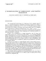
As shown by Tutte in [28], the structure resulting from the split operations is inde-
pendent of the order in which they are performed. It is a collection of graphs, called the
bricks of G, which are articulated around virtual edges, see Figure 4(b). By definition of
the decomposition, each brick has no split candidate; Tutte has shown that such graphs
are either multiedge-graphs (M-bricks) or ring-graphs (R-bricks), or 3-connected graphs
with at least 4 vertices (T-bricks).
The RMT-tree of G is the graph τ(G) whose nodes are the bricks of G and whose
edges correspond to the virtual edges of G (each virtual edge matches two bricks), see
Figure 4. The graph τ(G) is indeed a tree [28]. By maximality of the decomposition, it
is easily checked that τ(G) has no two R-bricks adjacent nor two M-bricks adjacent.
Call a brick-graph a graph that is either a ring-graph or a multi-edge graph or a 3-
the electronic journal of combinatorics 15 (2008), #R148 12
connected graph, with again the letter-triple {R, M, T } to refer to the type of the brick.
The inverse process of the split decomposition consists in taking a collection of brick-
graphs and a collection of edges, called virtual edges, so that each virtual edge belongs
to two bricks, and so that the graph τ with vertex-set the bricks and edge-set the virtual

edges (each virtual edge matches two bricks) is a tree avoiding two R-bricks or two M-
bricks being adjacent. Then the resulting graph, obtained by matching the bricks along
virtual edges and then erasing the virtual edges, is a 2-connected graph that has τ as its
RMT-tree. Hence, 2-connected graphs with at least 3 edges can be identified with their
RMT-tree, which again will be useful for writing down a decomposition grammar.
4.4 The restricted RMT-tree
The grammar to be written in Section 5 requires to decompose not only unrooted 2-
connected graphs, but also vertex-pointed 2-connected graphs. It turns out that these
vertex-pointed 2-connected graphs are much more convenient to decompose using a sub-
tree of the RMT-tree.
The restricted RMT-tree of a 2-connected graph G (with at least 3 edges) rooted at
a vertex v, is defined as the subgraph τ

(G) of the RMT-tree τ(G) induced by the bricks
containing v and by the edges of τ(G) connecting two such bricks.
Lemma 4.1. The restricted RMT-tree of a vertex-pointed 2-connected graph with at least
3 edges is a tree.
Proof. Let G be a vertex-pointed 2-connected graph with at least 3 edges. Let τ(G) be
the RMT-tree of G and let τ

(G) be the restricted RMT-tree of G. The pointed vertex is
denoted by v. As τ

(G) is a subgraph of the tree τ(G), it is enough to show that τ

(G)
is connected for it to be a tree. Recall that a virtual edge e corresponds to splitting G
into two graphs G
1
= G[E

1
] + e and G
2
= G[E
2
] + e, where E
1
, E
2
is a 2-separator of G.
The two subtrees T
1
and T
2
attached at each extremity of the virtual edge correspond to
the split-decomposition of G
1
and G
2
, respectively. Hence, the pointed vertex v, if not
incident to the virtual edge e, is either a vertex of G
1
\e or is a vertex of G
2
\e. In the first
(second) case, τ

(G) is contained in T
1
(T

2
, respectively). Hence, if an edge of τ(G) is not
in τ

(G), then τ

(G) does not overlap simultaneously with the two subtrees attached at
each extremity of that edge. This property ensures that τ

(G) is connected.
Having proved that the restricted RMT-tree is indeed a tree and not a forest, we will be
able to use the dissymmetry theorem—Theorem 3.1—in order to write a decomposition
grammar for the class of vertex-pointed 2-connected graphs. The restricted RMT-tree
turns out to be much better adapted for this purpose than the RMT-tree.
5 Decomposition Grammar
In this section we translate Tutte’s decomposition into an explicit grammar. Thanks to
this grammar, counting a family of graphs reduces to counting the 3-connected subfamily,
the electronic journal of combinatorics 15 (2008), #R148 13
which turns out to be a fruitful strategy in many cases, in particular for planar graphs,
as we will see Section 7.
Given a graph family G, our grammar corresponds at the first level to the connected
components, at the second level to the decomposition of a connected graph into 2-
connected blocks, and at the third level to the decomposition of a 2-connected graph
into 3-connected components. The first level is classic, the second level already makes use
of the dissymmetry theorem, it is implicitly used by Robinson [23], and appears explicitly
in the work by Leroux [18, 2]. The third level is new (though Leroux et al [13] have re-
cently independently derived general equation systems relating the series of 2-connected
graphs and 3-connected graphs of a given class). As we will see, it makes an even more
extensive use of the dissymmetry theorem than the second level.
We define the following subfamilies of G:

• The class G
1
is the subfamily of graphs in G that are connected and have at least
one vertex.
• The class G
2
is the subfamily of graphs in G that are 2-connected and have at least
two vertices. Multiple edges are allowed. (The smallest possible such graph is the
link-graph that has two vertices connected by one edge.)
• The class G
3
is the subfamily of graphs in G that are 3-connected and have at least
four vertices. (The smallest possible such graph is the tetrahedron.)
A class G of graphs is said to be stable under Tutte’s decomposition if it satisfies the
following property:
“any graph G is in G iff all 3-connected components of G are in G”.
Notice that a class of graphs stable under Tutte’s decomposition satisfies the following
properties:
• a graph G is in G iff all its connected components are in G
1
,
• a graph G is in G
1
iff all its 2-connected components are in G
2
,
• a graph G is in G
2
iff all its 3-connected components are in G
3

.
5.1 General from connected graphs
The first level of the grammar is classic. A graph is simply the collection of its connected
components, which translates to:
G = Set(G
1
). (6)
the electronic journal of combinatorics 15 (2008), #R148 14
5.2 Connected from 2-connected graphs
In order to write down the second level, i.e., decompose the connected class C := G
1
, we
define the following classes: C
B
is the class of graphs in G
1
with a distinguished block, C
v
is the class of graphs in G
1
with a distinguished vertex, and C
Bv
is the class of graphs in G
1
with a distinguished incidence block-vertex. In other words, C
B
, C
v
, and C
Bv

correspond
to graphs in G
1
where one distinguishes in the associated Bv-tree, respectively, a v-node, a
B-node, and an edge. The generalized dissymmetry theorem yields the following relation
between C = G
1
and the auxiliary rooted classes:
C + C
Bv
= C
v
+ C
B
,
which can be rewritten as
C = C
v
+ C
B
− C
Bv
. (7)
Clearly the class C

is related to C
v
by C
v
= v ∗ C


. To decompose C

, we observe that
the pointed vertex gives a starting point for a recursive decomposition. Precisely, from the
block decomposition described in Section 4.2, any vertex-pointed connected graph is ob-
tained as follows: take a collection of vertex-pointed 2-connected graphs attached together
at their marked vertices, and attach a vertex-pointed connected graph at each non-pointed
vertex of these 2-connected graphs. (Clearly the 2-connected graphs correspond to the
blocks incident to the pointed vertex in the resulting graph.)
This recursive decomposition translates to the equation
C

= Set(G
2

◦
v
C

). (8)
Similarly, each graph in C
B
is obtained in a unique way by taking a block in G
2
and
attaching at each vertex of the block a vertex-pointed connected graph in C

, which yields
C

B
= G
2
◦
v
C

. (9)
Finally, each graph in C
Bv
is obtained from a vertex-pointed block in G
2

by attaching
at each vertex of the block —even the root vertex— a vertex-pointed connected graph,
which yields
C
Bv
= (v ∗ G
2

) ◦
v
C

. (10)
The grammar to decompose a class of connected graphs into 2-connected components
results from the concatenation of Equations (7), (8), (9), and (10).
A similar grammar is given in the book of Bergeron, Labelle and Leroux [2]. Notice
that there are two terminal classes in this grammar, the class G

2
and the class G
2

.
5.3 2-Connected from 3-connected graphs
In this section we start to describe the new contributions of this article, namely the
decomposition grammars for G
2
and G
2

.
Let us begin with G
2
. Again we have to define auxiliary classes that correspond to
the different ways to distinguish a node or an edge in the RMT-tree. Let B be the class
the electronic journal of combinatorics 15 (2008), #R148 15
of graphs in G
2
with at least 3 edges (i.e., those whose RMT-tree is not empty). Since
we consider graph classes stable under Tutte’s decomposition, the link-graph 
1
and the
double-link graph 
2
(which have counting series x
2
y/2 and x
2

y
2
/2, respectively) are in
G
2
, hence
G
2
= 
1
+ 
2
+ B. (11)
Next we decompose B using the RMT-tree. Let B
◦
(B
◦−◦
, B
◦→◦
) be the class of graphs
in B such that the RMT-tree carries a distinguished node (edge, directed edge, resp.).
Theorem 3.1 yields
B = B
◦
+ B
◦−◦
− B
◦→◦
. (12)
The class B

◦
is naturally partitioned into 3 classes B
R
, B
M
, and B
T
, depending on the
type of the distinguished node (R-node, M-node, or T-node). Similarly, the class B
◦−◦
is
partitioned into 4 classes B
R−M
, B
R−T
, B
M−T
, and B
T −T
(recall that a RMT-tree has no
two adjacent R-bricks nor two adjacent M-bricks); and B
◦→◦
is partitioned into 7 classes
B
R→M
, B
M→R
, B
R→T
, B

T →R
, B
M→T
, B
T →M
, and B
T →T
. Notice that B
R→M
 B
M→R

B
R−M
, B
R→T
 B
T →R
 B
R−T
, and B
M→T
 B
T →M
 B
M−T
. Hence, Equation (12) is
rewritten as
B = B
R

+ B
M
+ B
T
− B
R−M
− B
R−T
− B
M−T
− B
T →T
+ B
T −T
. (13)
5.3.1 Networks
In order to decompose the classes on the right-hand-side of Equation (13), we first have to
decompose the class of rooted 2-connected graphs in G, more precisely we need to specify a
grammar for a class of objects closely related to
−→
G
2
, which are called networks. A network
is defined as a connected graph arising from a graph in
−→
G
2
by deleting the root-edge; the
origin and end of the root-edge are respectively called the 0-pole and the ∞-pole of the
network. The associated class is classically denoted by D in the literature [29]. Observe

that the only rooted 2-connected graph disconnected by root-edge deletion is the rooted
link-graph. Hence
−→
G
2
= 1 + D,
where the rooted link-graph has weight 1 instead of e because, in a rooted class, the rooted
edge is considered as unlabelled, i.e., is not counted in the size parameters. (We will see
in Section 5.4 that the link between D and
−→
G
2
is a bit more complicated if multiple edges
are forbidden.)
As discovered by Tracktenbrot [26] a few year’s before Tutte’s book appeared, the class
of networks with at least 2 edges (recall that the root-edge has been deleted) is naturally
partitioned into 3 subclasses: S for series networks, P for parallel networks, and H for
polyhedral networks:
D = e + S + P + H. (14)
With our terminology of RMT-tree, the three situations correspond to the root-edge
the electronic journal of combinatorics 15 (2008), #R148 16
belonging to a R-brick, M-brick, or T-brick, respectively
2
. In a similar way as for the
class G
1

in Section 5.2, the root-edge gives a starting point for a recursive decomposition.
Clearly, as there is no edge R-R in the RMT-tree, each series network is obtained as
a collection of at least two non-series networks connected as a chain (the ∞-pole of a

network is identified with the 0-pole of the following network in the chain):
S = (D − S) ∗v ∗ D. (15)
Similarly, as there is no edge M-M in the RMT-tree, each parallel-network is obtained as
a collection of at least two non-parallel networks sharing the same 0- and ∞-poles:
P = Set
≥2
(D − P). (16)
Finally, each polyhedral network is obtained as a rooted 3-connected graph where each
non-root edge is substituted by a network, which yields:
H =
−→
G
3
◦
e
D. (17)
The resulting decomposition grammar for D is obtained as the concatenation of Equa-
tions (14), (15), (16), and (17). This grammar has been known since Walsh [29]. Notice
that the only terminal class is the 3-connected class
−→
G
3
.
5.3.2 Unrooted 2-connected graphs
We can now specify the decompositions of the families on the right-hand-side of (13).
Recall that R is the class of ring-graphs (polygons) and M is the class of multiedge
graphs with at least 3 edges. Given a graph in B
R
, each edge e of the distinguished R-
brick is either a real edge or a virtual edge; in the latter case the graph attached on the

other side of e (i.e., the side not incident to the rooted R-brick) is naturally rooted at e;
it is thus identified with a network (upon choosing an orientation of e), precisely it is a
non-series network, as there are no two R-bricks adjacent. Hence
B
R
= R ◦
e
(D − S). (18)
Similarly we obtain
B
M
= M ◦
e
(D − P) = (v
2
∗ Set
≥3
(D − P))/•  •, (19)
where the last notation means “up to exchanging the two pole-vertices of the multiedge
component”, and
B
T
= G
3
◦
e
D, (20)
to be compared with H =
−→
G

3
◦
e
D. Next we decompose 2-connected graphs with a
distinguished edge in the RMT-tree. Consider the class B
R−M
. The distinguished edge of
2
Actually Trackhtenbrot’s decomposition can be seen as Tutte’s decomposition restricted to rooted
2-connected graphs.
the electronic journal of combinatorics 15 (2008), #R148 17
the RMT-tree corresponds to a virtual edge {u, v} matching one R-brick and one M-brick,
such that the two bricks are attached at {u, v}. Upon fixing an orientation of the virtual
edge {u, v}, there is a series-network on one side of {u, v} and a parallel-network on the
other side. Notice that such a construction has to be considered up to orienting {u, v},
i.e., up to exchanging the two poles u and v (notation /•  •). We obtain
B
R−M
= (S ∗P)/•  •. (21)
Similarly,
B
M−T
= (P ∗H)/•  •, B
R−T
= (S ∗H)/•  •, B
T →T
= (H ∗H)/•  •,
B
T −T
= (H ∗ H)/(•  •, H  H),

where the very last notation means “up to orienting the distinguished virtual edge”.
5.3.3 Vertex-pointed 2-connected graphs
Now we decompose the class G
2

of vertex-pointed 2-connected graphs (recall that G
2

is,
with G
2
, one of the two terminal classes in the decomposition grammar for connected
graphs into 2-connected components). We proceed in a similar way as for G
2
, with the
important difference that we use the restricted RMT-tree instead of the RMT-tree. Ob-
serve that the class of graphs in G
2

with at least 3 edges (those whose RMT-tree is not
empty) is the derived class V := B

. By deriving the identity (11), we get
G
2

= 
1

+ 

2

+ V = v ∗ e + v ∗ Set
2
(e) + V. (22)
We denote by V
◦
(V
◦−◦
, V
◦→◦
) the class of graphs in G
2

where the associated restricted
RMT-tree carries a distinguished node (edge, oriented edge, resp.). Theorem 3.1 yields
V = V
◦
+ V
◦−◦
− V
◦→◦
. (23)
Notice that V
◦
= (B
◦
)

, V

◦−◦
= (B
◦−◦
)

, and V
◦→◦
= (B
◦→◦
)

, due to the fact that the
associated tree is not the same for V = B

and for B (actually, taking the derivative of
the grammar for B would produce a much more complicated grammar for B

than the
one we will obtain using the restricted RMT-tree). We partition the classes V
◦
, V
◦−◦
,
and V
◦→◦
according to the types of the bricks incident to the root, and proceed with a
decomposition in each case; the arguments are very similar as for the decomposition of
G
2
. Take the example of V

T
. Since the pointed vertex of the graph is incident to the
marked T-brick (this is where it is very nice to consider the restricted RMT-tree instead
of the RMT-tree), we have
V
T
= G
3

◦
e
D,
to be compared with B
T
= G
3
◦
e
D. Similarly we obtain
V
R
= R

◦
e
(D − S), V
M
= M

◦

e
(D − P) = v ∗ Set
≥3
(D − P),
V
R−M
= v ∗ S ∗ P, V
R−T
= v ∗ S ∗ H, V
M−T
= v ∗ P ∗ H,
V
T →T
= v ∗ H ∗ H, V
T −T
= (v ∗ H ∗ H)/H  H.
We have now a generic grammar to decompose a family of graphs into 3-connected
components; the complete grammar is shown in Figure 6, and the main dependencies are
shown in Figure 5. Observe that, except for the easy basic classes v, e, 
1
, 
2
, Set
≥k
, R,
M, R

, M

, the only terminal classes are the 3-connected classes G

3
, G

3
, and
−→
G
3
.
the electronic journal of combinatorics 15 (2008), #R148 18
G
3
−→
G
3
G
3

D
G
2

G
2
G
1

G
1
G

Figure 5: The main dependencies in the grammar.
5.4 Adapting the grammar for families of simple graphs
The grammar has been described for a family G satisfying the stability condition under
Tutte’s decomposition, and where multi-edges are allowed. It is actually very easy to
adapt the grammar for the corresponding simple family of graphs. Call G the subfamily
of graphs in G that have no multiple edges and G
1
, G
2
, G
3
the corresponding subfamilies
of connected, 2-connected, and 3-connected graphs.
To write down a grammar for G we just need to trace where the multiple edges might
appear in the decomposition grammar for G. Clearly a graph is simple iff all its 2-
connected components are simple, so we just need to look at the last part of the grammar:
2-connected from 3-connected. Among the two 2-connected graphs with less than 3 edges
(the family ), we have to forbid the double-link graph, i.e., we have to take  = 
2
instead
of  = 
1
+ 
2
. Among the 2-connected graphs with at least 3 edges—those giving rise
to a RMT-tree—we have to forbid those where some M-brick has at least 2 components
that are edges (indeed all representatives of a multiple edge are components of a same
M-brick, so we can characterize the absence of multiple edges directly on the RMT-tree).
Accordingly we have to change the specifications of the classes involving the decomposition
at an M-brick, i.e., the classes P, B

M
, and V
M
. In each case we have to distinguish if there
is one edge component or zero edge-component incident to the M-brick, so there are two
terms for the decomposition of each these families. For the class P of parallel networks, we
have now P = e ∗Set
≥1
(D−P −e) +Set
≥2
(D−P −e) instead of P = Set
≥2
(D−P). For
the class B
M
, we have now B
M
= (v
2
∗e ∗Set
≥2
(D−P −e) + v
2
∗Set
≥3
(D−P −e))/•  •
instead of B
M
= (v
2

∗ Set
≥3
(D − P))/•  •. And for the class V
M
, we have now
V
M
= v ∗e ∗Set
≥2
(D−P −e) + v ∗Set
≥3
(D−P −e) instead of V
M
= v ∗Set
≥3
(D−P).
These are indicated in the grammar (Figure 6).
the electronic journal of combinatorics 15 (2008), #R148 19
(1). General from Connected (folklore).
G = Set(G
1
)
(2). Connected from 2-Connected (Bergeron, Labelle, Leroux).
G
1
= C = C
v
+ C
B
− C

Bv
[dissymmetry theorem]
C
v
= v ∗ C

C

= Set(G
2

◦
v
C

)
C
B
= G
2
◦
v
C

C
Bv
= (v ∗ G
2

) ◦

v
C

(3). 2-Connected from 3-Connected.
(i) Networks
D = e + S + P + H
S = (D − S) ∗ v ∗ D
P =

Set
≥2
(D − P), [Multi-edges allowed]
e ∗ Set
≥1
(D − P − e) + Set
≥2
(D − P − e), [No Multi-edges]
H =
−→
G
3
◦
e
D
(ii) Unrooted 2-Connected
G
2
=  + B,  =



1
+ 
2
[Multi-edges allowed]

1
[No multi-edges]
B = B
R
+ B
M
+ B
T
− B
R−M
− B
R−T
− B
M −T
− B
T →T
+ B
T −T
B
R
= R ◦
e
(D − S)
B
M

=

M ◦
e
(D − P) = (v
2
∗ Set
≥3
(D − P))/•  •, [Multi-edges allowed]
(v
2
∗ e ∗ Set
≥2
(D − P − e) + v
2
∗ Set
≥3
(D − P − e))/•  •, [No multi-edges]
B
T
= G
3
◦
e
D
B
R−M
= (v
2
∗ S ∗ P )/•  •, [Up to pole exchange, denoted by /•  •]

B
R−T
= (v
2
∗ S ∗ H)/•  •
B
M −T
= (v
2
∗ P ∗ H)/•  •
B
T →T
= (v
2
∗ H ∗ H)/•  •
B
T −T
= (v
2
∗ H ∗ H)/(•  •, H  H), [Up to pole and component exchange]
(iii) Vertex-pointed 2-Connected
G
2

= 

+ B

, 


=


1

+ 
2

= v ∗ (e + Set
2
(e)) [Multi-edges allowed]

1

= v ∗ e [No multi-edges]
B

= V = V
R
+ V
M
+ V
T
− V
R−M
− V
R−T
− V
M −T
− V

T →T
+ V
T −T
V
R
= R

◦
e
(D − S)
V
M
=

v ∗ Set
≥3
(D − P), [Multi-edges allowed]
v ∗ e ∗ Set
≥2
(D − P − e) + v ∗ Set
≥3
(D − P − e), [No multi-edges]
V
T
= G
3

◦
e
D

V
R−M
= v ∗ S ∗ P
V
R−T
= v ∗ S ∗ H
V
M −T
= v ∗ P ∗ H
V
T →T
= v ∗ H ∗ H
V
T −T
= (v ∗ H ∗ H)/H  H
Figure 6: The grammar to decompose a graph family G stable under Tutte’s decomposi-
tion. The non-basic terminal classes of the grammar are the 3-connected classes G
3
, G
3

,
and

G
3
.
the electronic journal of combinatorics 15 (2008), #R148 20
(1). General from Connected (folklore).
G(z, y) = exp(G

1
(z, y))
(2). Connected from 2-Connected (Bergeron, Labelle, Leroux).
[The variables z and x are related by x = zG
1

(z, y).]
G
1
(z, y) = C(z, y) = C
v
(z, y) + C
B
(z, y) − C
vB
(z, y)
C
v
(z, y) = zC

(z, y)
C

(z, y) = exp (G
2

(x, y))
C
B
(z, y) = G

2
(x, y)
C
vB
(z, y) = xG
2

(x, y)
(3). 2-Connected from 3-Connected.
[The variables y and w are related by w = D(x, y).]
[We use the notations exp
≥k
(t) = exp(t) −
k−1

i=1
t
i
i!
and loga
≥k
(t) = log(1/(1 − t)) −
k−1

i=1
t
i
i
.]
(i) Networks

D(x, y) = y + S(x, y) + P (x, y) + H(x, y)
S(x, y) = (D(x, y) − S(x, y))xD(x, y)
P (x, y) =

exp
≥2
(D(x, y) − P (x, y)) [Multi-edges]
y exp
≥1
(D(x, y) − P (x, y) − y) + exp
≥2
(D(x, y) − P (x, y) − y) [No Multi-edges]
H(x, y) =
−→
G
3
(x, w)
(ii) Unrooted 2-Connected
G
2
(x, y) = (x, y) + B(x, y), (x, y) =

x
2
(y/2 + y
2
/4) [Multi-edges]
x
2
y/2 [No multi-edges]

B(x, y) = B
R
(x, y)+B
M
(x, y)+B
T
(x, y)−B
R−M
(x, y)−B
R−T
(x, y)−B
M −T
(x, y)−B
T −T
(x, y)
B
R
(x, y) = loga
≥3
(x · (D(x, y)−S(x, y)))/2
B
M
(x, y) =

x
2
exp
≥3
(D(x, y) − P (x, y))/2, [Multi-edges]
x

2

y exp
≥2
(D(x, y)−P (x, y)−y)+exp
≥3
(D(x, y)−P (x, y)−y)

/2, [No multi-edges]
B
T
(x, y) = G
3
(x, w)
B
R−M
(x, y) = x
2
S(x, y) · P (x, y)/2
B
R−T
(x, y) = x
2
S(x, y) · H(x, y)/2
B
M−T
(x, y) = x
2
P (x, y) · H(x, y)/2
B

T −T
(x, y) = x
2
H(x, y)
2
/4
(iii) Vertex-pointed 2-Connected
G
2

(x, y) = 

(x, y) + B

(x, y), 

(x, y) =

x(y + y
2
/2) [Multi-edges]
xy [No multi-edges]
B

(x, y) = V
R
(x, y)+V
M
(x, y)+V
T

(x, y)−V
R−M
(x, y)−V
R−T
(x, y)−V
M −T
(x, y)−V
T −T
(x, y)
V
R
(x, y) = x
2
(D(x, y) − S(x, y))
2
D(x, y)/2
V
M
(x, y) =

x exp
≥3
(D(x, y)−P (x, y)), [Multi-edges]
xy exp
≥2
(D(x, y)−P (x, y)−y) + x exp
≥3
(D(x, y)−P (x, y)−y), [No multi-edges]
V
T

(x, y) = G
3

(x, w)
V
R−M
(x, y) = xS(x, y) · P (x, y)
V
R−T
(x, y) = xS(x, y) · H(x, y)
V
M−T
(x, y) = xP (x, y) · H(x, y)
V
T −T
(x, y) = xH(x, y)
2
/2
Figure 7: The equation-system to express the series counting a family of graphs in terms of
the series counting the 3-connected subfamilies (the terminal series are G
3
(x, w), G
3

(x, w),

G
3
(x, w)) is obtained by translating the grammar shown in Figure 6.
the electronic journal of combinatorics 15 (2008), #R148 21

6 Application: counting a graph family reduces to
counting the 3-connected subfamily
At first notice that our grammar makes it possible to get an exact enumeration procedure
for a graph family G (stable under Tutte’s decomposition) from the counting coefficients
of the 3-connected subfamily, whether in the labelled or in the unlabelled setting. For
instance, Figure 7 shows the translation of the grammar into an equation system for the
corresponding exponential generating functions (for labelled enumeration). To get the
counting coefficients, one can either turn this system into recurrences (see [5] for the
precise recurrences) or simply compute Taylor developments of increasing degree in an
inductive way. For doing all this, a partial decomposition grammar (allowing integrals)
is actually enough, since formal integration just means dividing the nth coefficient by n.
The purpose of this section is to stress the relevance of our grammar in order to get
analytic expressions for series counting families of graphs, thereby making it possible—
via the techniques of singularity analysis—to get precise asymptotic results. (The latter
point, singularity analysis, is not treated in this article, see [15, 14] for a detailed study.)
Precisely, we show that finding an (implicit) analytic expression for a series counting
a family of graphs stable under Tutte’s decomposition reduces to finding an analytic
expression for the series counting the 3-connected subfamily, a task that is easier in many
cases, in particular for planar graphs, see Section 7.
Let us mention that Gim´enez, Noy, and Ru´e have recently shown in [14] that their
method, which involves integrations, also makes it possible to have general equation sys-
tems relating the series counting a family of graphs and the series counting the 3-connected
subfamilies. Hence we do not claim originality here, we only point out that the equation
system can be derived automatically from a grammar, without using analytic integrations.
Definition 6.1. A multivariate power series C := C(z) is said to be analytically specified
if it is of the following form (notice that the definition is inductive and relies heavily on
substitutions).
Initial level. Rational generating functions (in any number of variables), the log function,
and the exp function are analytically specified.
Incremental definition. Let C = F

1
be a power series that is uniquely specified by a system
of the form





F
1
= Expression
1
,
.
.
.
F
m
= Expression
m
,
(24)
each expression being of the form G(H
1
, . . . , H
k
), where G is a series already known to
be analytically specified, and where each H
i
is either equal to one of the F

j
’s or is a series
already known to be analytically specified. Then C is declared to be analytically specified
as well.
Analytically specified series are typically amenable to singularity analysis techniques
in order to obtain precise asymptotic informations (enumeration, limit laws of parameters
the electronic journal of combinatorics 15 (2008), #R148 22
on a random instance); let us review briefly how the method works. Given a series C
specified by a system of the form (24), one has to consider the dependency graph between
the F
i
’s, in particular the strongly connected components of that graph. Notice that some
of the F
i
’s are expressed in (24) as a substitution in terms of functions already known to
be analytically specified; in that case one would also include the dependency graph for
the specification of this series, at a lower level. Therefore one gets a global dependency
graph for C that is a hierarchy of dependency graphs (one for each specifying system).
Then one treats the strongly components of this global dependency graph “from bot-
tom to top”, tracing the singularities on the way. In general, singularities are either due
to the Jacobian of the system vanishing (for “tree-like” singularities, see the Drmota-
Lalley-Woods theorem [9, sec VII.6]) or stem from a singularity of a function in a lower
strongly connected component. Recently the techniques of singularity analysis have been
successfully applied to the class of planar graphs by Gim´enez and Noy [15], building on
earlier results by Bender, Gao, and Wormald [1]. One important difficulty in their work
was to actually obtain a system of equations specifying planar graphs without integration
operator, since integrations make it difficult to trace the singularities (in particular when
several variables are involved).
We prove here that our grammar provides a direct combinatorial way to obtain such
a system of equations for planar graphs. Thanks to our grammar, finding an (implicit)

expression for the series counting a graph family G (stable under Tutte’s decomposition)
reduces to finding an (implicit) expression for the series counting the 3-connected sub-
family G
3
.
Theorem 6.1. Let G be a family of graphs satisfying the stability condition (i.e., a graph
is in G iff its 3-connected components are also in G). Call G
3
the 3-connected subfamily
of G, and denote respectively by G(x, y) and G
3
(x, y) the (exponential) counting series
for the classes G and G
3
, where x marks the vertices and y marks the edges. Assume
that G
3
(x, y) is analytically specified. Then G(x, y) is also analytically specified via the
equation-system shown in Figure 7 and the analytic specification for G
3
(x, y).
Proof. Assume that G
3
is analytically specified. At first let us mention the following
simple lemma: if a series C is analytically specified then any of its partial derivatives is also
analytically specified; this is due to the fact that one can “differentiate” the specification
for C. (For the sake of illustration, take the univariate series for binary trees: B(x) =
x+B(x)
2
. Then the derivative B


(x) satisfies the system {B

(x) = 1+2B

(x)B(x), B(x) =
x + B(x)
2
}.) Hence, the series G
3

and
−→
G
3
are also analytically specified.
Now notice that G
3
, G
3

and
−→
G
3
are (together with elementary functions such as log) the
only terminal series in the equation-system shown in Figure 7. In addition, this system
clearly satisfies the requirements of an analytic specification. One shows successively
“from bottom to top” that the series for the following graph classes are analytically
specified: networks, unrooted 2-connected, vertex-pointed 2-connected, vertex-pointed

connected, connected, and general graphs in the family one considers.
the electronic journal of combinatorics 15 (2008), #R148 23
7 The series counting labelled planar graphs can be
specified analytically
This section is dedicated to proving the following result.
Theorem 7.1. The series counting labelled planar graphs w.r.t. vertices and edges is
analytically specified.
Theorem 7.1 has already been proved by Gim´enez and Noy [15] (as a crucial step to
enumerate planar graphs asymptotically). Our contribution is a more straightforward
proof of this result, which uses only combinatorial arguments and elementary algebraic
manipulations; the main ingredients are our grammar and a bijective construction of
vertex-pointed maps. In this way we avoid the technical integration steps addressed
in [15].
Let us give a more precise outline of our proof. At first we take advantage of the
grammar; the class of planar graphs satisfies the stability condition (planarity is preserved
by taking the 3-connected components), hence proving Theorem 7.1 reduces (by Theo-
rem 6.1) to finding an analytic specification for the series G
3
(x, w) counting 3-connected
planar graphs, which is the task we address from now on.
By a theorem of Whitney [32], 3-connected planar graphs have a unique embedding on
the sphere (up to reflections), hence counting 3-connected planar graphs is equivalent to
counting 3-connected maps (up to reflections). To solve the latter problem, we combine
several tools. Firstly, the Euler relation makes it possible to reduce the enumeration of
3-connected maps to the enumeration of vertex-pointed 3-connected maps; secondly a
bijective construction due to Bouttier et al [7] allows us to count unrestricted vertex-
pointed maps; finally a suitable adaptation of our grammar used in a top-to-bottom way
yields the enumeration of vertex-pointed 3-connected maps via vertex-pointed 2-connected
maps.
7.1 Maps

A map is a connected graph planarly embedded on the sphere up to continuous defor-
mation. All maps considered here have at least one edge. As opposed to graphs, loops
are allowed on arbitrary maps (as well as multi-edges). Thus, under Tutte’s definition, a
2-connected map is either the loop-map, or is a loopless map with no separating vertex.
Similarly as for graphs, a map is rooted if one of its edges is marked and oriented, and
a map is vertex-pointed if one of its vertices is marked. An important remark is that
rooting a map is equivalent to marking one of its corners (indeed there is a one-to-one
correspondence between the corners and the half-edges of a map). We use the following
notations:
•
−→
M(x, s) and M

(x, s) are the series counting respectively rooted maps and vertex-
pointed maps, where x marks the number of vertices minus one (say, the root vertex
for
−→
M, the pointed vertex for M

), and s marks the number of half-edges. Here
the electronic journal of combinatorics 15 (2008), #R148 24
vertices are unlabelled and half-edges are labelled (this is enough to avoid any
symmetry), hence the series are exponential w.r.t. half-edges and ordinary w.r.t.
vertices.
• Similarly,
−→
L (x, s), and L

(x, s) are the series counting rooted 2-connected maps
and vertex-pointed 2-connected maps respectively, where x marks the number of

(unlabelled) vertices minus one, and s marks the number of (labelled) half-edges.
• Finally, K(x, w) (
−→
K(x, w), K

(x, w)) are the series of unrooted (rooted, vertex-
pointed, resp.) 3-connected maps with at least 4 vertices. Contrary to maps and
2-connected maps, the conventions are exactly the same as for graphs, i.e., x marks
labelled vertices (which carry blue labels) and w marks labelled edges (which carry
red labels); the marked vertex is unlabelled for maps counted by K

(x, w), and the
root-edge and its ends are unlabelled for maps counted by
−→
K(x, w).
7.2 Reduction to counting vertex-pointed 3-connected maps
At first we recall Whitney’s theorem [31]: every 3-connected planar graph has a unique
embedding on the sphere up to reflection. Since a 3-connected map with at least 4 vertices
differs from its mirror-image, each planar graph in G
3
gives rise to exactly two maps, which
yields
G
3
(x, w) =
1
2
K(x, w). (25)
Next, the task of finding an expression for K(x, w) is reduced to finding an expression for
the series counting vertex-pointed 3-connected maps. Let K

V
(x, w), K
E
(x, w), K
F
(x, w)
be the series counting respectively vertex-pointed, edge-pointed, and face-pointed 3-
connected maps (here all vertices and all edges are labelled). The Euler relation (i.e.,
1 = 1/2 · (|vertices| − |edges| + |faces|)) yields
K(x, w) =
1
2
(K
V
(x, w) − K
E
(x, w) + K
F
(x, w)).
The series K
E
corresponds to half the series counting rooted 3-connected planar maps,
which has been obtained by Mullin and Schellenberg [21] (we review briefly the compu-
tation scheme in Section 7.5.1) and more recently in a bijective way in [11]:
K
E
(x, w) =
1
2
x

2
w
−→
K(x, w) =
1
2
x
2

w −
xw
2
1 + xw
−
w
2
1 + w
−
γ
1
γ
2
xw(1 + γ
1
+ γ
2
)
3

,

where γ
1
= γ
1
(x, w) and γ
2
= γ
2
(x, w) are specified by the system
γ
1
= xw(1 + γ
2
)
2
, γ
2
= w(1 + γ
1
)
2
.
Moreover, as the class of 3-connected maps is well known to be stable by duality, we have
(using again the Euler relation)
K
F
(x, w) = x
2
K
V

(1/x, xw).
the electronic journal of combinatorics 15 (2008), #R148 25