Báo cáo toán học: "Ternary linear codes and quadrics" docx
Bạn đang xem bản rút gọn của tài liệu. Xem và tải ngay bản đầy đủ của tài liệu tại đây (201.24 KB, 21 trang )
Ternary linear codes and quadrics
Yuri Yoshida and Tatsuya Maruta
∗
Department of Mathematics and Information Sciences
Osaka Prefecture University, Sakai, Osaka 599-8531, Japan
,
Submitted: Dec 4, 2008; Accepted: Jan 7, 2009; Published: Jan 16, 2009
Mathematics Subject Classification: 94B27, 94B05, 51E20, 05B25
Abstract
For an [n, k, d]
3
code C with gcd(d, 3) = 1, we define a map w
G
from Σ =
PG(k − 1, 3) to the set of weights of codewords of C through a generator matrix
G. A t-flat Π in Σ is called an (i, j)
t
flat if (i, j) = (|Π ∩ F
0
|, |Π ∩ F
1
|), where
F
0
= {P ∈ Σ | w
G
(P ) ≡ 0 (mod 3)}, F
1
= {P ∈ Σ | w
G
(P ) ≡ 0, d (mod 3)}.
We give geometric characterizations of (i, j)
t
flats, which involve quadrics. As an
application to the optimal linear codes problem, we prove the non-existence of a
[305, 6, 202]
3
code, which is a new result.
1 Introduction
Let F
n
q
denote the vector space of n-tuples over F
q
, the field of q elements. A linear code
C of length n, dimension k and minimum (Hamming) distance d over F
q
is referred to as
an [n, k, d]
q
code. Linear codes over F
2
, F
3
, F
4
are called binary, ternary and quaternary
linear codes, respectively. The weight of a vector x ∈ F
n
q
, denoted by wt(x), is the number
of nonzero coordinate positions in x. The weight distribution of C is the list of numbers
A
i
which is the number of codewords of C with weight i. The weight distribution with
(A
0
, A
d
, ) = (1, α, ) is also expressed as 0
1
d
α
· · · . We only consider non-degenerate
codes having no coordinate which is identically zero. An [n, k, d]
q
code C with a generator
matrix G is called (l, s)-extendable (to C
) if there exist l vectors h
1
, . . . , h
l
∈ F
k
q
so that
the extended matrix [G, h
T
1
, · · · , h
T
l
] generates an [n + l, k, d + s]
q
code C
([10]). Then C
is called an (l, s)-extension of C. C is simply called extendable if C is (1, 1)-extendable.
We denote by PG(r, q) the projective geometry of dimension r over F
q
. A j-flat is
a projective subspace of dimension j in PG(r, q). 0-flats, 1-flats, 2-flats, 3-flats, (r − 2)-
flats and (r − 1)-flats are called points, lines, planes, solids, secundums and hyperplanes,
∗
This research was partially supported by Grant-in-Aid for Scientific Research of Japan Society for
the Promotion of Science under Contract Number 20540129.
the electronic journal of combinatorics 16 (2009), #R9 1
respectively. We refer to [7], [8] and [9] for geometric terminologies. We investigate linear
codes over F
q
through the projective geometry.
We assume that k ≥ 3. Let C be an [n, k, d]
q
code with a generator matrix G =
[g
0
, g
1
, · · · , g
k−1
]
T
. Put Σ =PG(k − 1, q), the projective space of dimension k − 1 over F
q
.
We consider the mapping w
G
from Σ to {i | A
i
> 0}, the set of weights of codewords of
C. For P = P(p
0
, p
1
, . . . , p
k−1
) ∈ Σ we define the weight of P with respect to G, denoted
by w
G
(P ), as
w
G
(P ) = wt(
k−1
i=0
p
i
g
i
).
Our geometric method is just the dual version of that introduced first in [11] to investigate
the extendability of C. See also [14], [15], [16], [18] for the extendability of ternary linear
codes. Let
F = {P ∈ Σ | w
G
(P ) ≡ d (mod q)},
F
d
= {P ∈ Σ | w
G
(P ) = d}.
Recall that a hyperplane H of Σ is defined by a non-zero vector h = (h
0
, . . . , h
k−1
) ∈ F
k
q
as H = {P = P(p
0
, . . . , p
k−1
) ∈ Σ | h
0
p
0
+ · · · + h
k−1
p
k−1
= 0}. h is called a defining
vector of H, which is uniquely determined up to non-zero multiple. It would be possible
to investigate the (l, 1)-extendability of linear codes from the geometrical structure of F
or F
d
as follows.
Theorem 1.1 ([12]). C is (l, 1)-extendable if and only if there exist l hyperplanes H
1
, . . .,
H
l
of Σ such that F
d
∩ H
1
∩ · · · ∩ H
l
= ∅. Moreover, the extended matrix of G by adding
the defining vectors of H
1
, . . . , H
l
as columns generates an (l, 1)-extension of C. Hence, C
is (l, 1)-extendable if there exists a (k − 1 − l)-flat contained in F .
The mapping w
G
is trivial if F = ∅. For example, w
G
is trivial if C attains the Griesmer
bound and if q divides d when q is prime [17]. When w
G
is trivial, there seems no clue
to investigate the extendability of C except for computer search, see [10]. To avoid such
cases we assume gcd(d, q) = 1; d and q are relatively prime. Then, F forms a blocking
set with respect to lines [12], that is, every line meets F in at least one point. The aim of
this paper is to give a geometric characterization of F for q = 3. An application to the
optimal linear codes problem is also given in Section 4.
2 Main theorems
Let C be an [n, k, d]
3
code with k ≥ 3, gcd(3, d) = 1. The diversity (Φ
0
, Φ
1
) of C was
defined in [11] as the pair of integers:
Φ
0
=
1
2
3|i,i=0
A
i
, Φ
1
=
1
2
i≡0,d (mod 3)
A
i
,
the electronic journal of combinatorics 16 (2009), #R9 2
where the notation x|y means that x is a divisor of y. Let
F
0
= {P ∈ Σ | w
G
(P ) ≡ 0 (mod 3)},
F
2
= {P ∈ Σ | w
G
(P ) ≡ d (mod 3)},
F
1
= F \ F
0
, F
e
= F
2
\ F
d
.
Then we have Φ
s
= |F
s
| for s = 0, 1.
A t-flat Π of Σ with |Π ∩ F
0
| = i, |Π ∩ F
1
| = j is called an (i, j)
t
flat. An (i, j)
1
flat
is called an (i, j)-line. An (i, j)-plane, an (i, j)-solid and so on are defined similarly. We
denote by F
j
the set of j-flats of Σ. Let Λ
t
be the set of all possible (i, j) for which an
(i, j)
t
flat exists in Σ. Then we have
Λ
1
= {(1, 0), (0, 2), (2, 1), (1, 3), (4, 0)},
Λ
2
= {(4, 0), (1, 6), (4, 3), (4, 6), (7, 3), (4, 9), (13, 0)},
Λ
3
= {(13, 0), (4, 18), (13, 9), (10, 15), (16, 12), (13, 18), (22, 9), (13, 27), (40, 0)},
Λ
4
= {(40, 0), (13, 54), (40, 27), (31, 45), (40, 36), (40, 45), (49, 36), (40, 54), (67, 27),
(40, 81), (121, 0)},
Λ
5
= {(121, 0), (40, 162), (121, 81), (94, 135), (121, 108), (112, 126), (130, 117),
(121, 135), (148, 108), (121, 162), (202, 81), (121, 243), (364, 0)},
see [11]. Let Π
t
∈ F
t
. Denote by c
(t)
i,j
the number of (i, j)
t−1
flats in Π
t
and let ϕ
s
(t)
=
|Π
t
∩ F
s
|, s = 0, 1. (ϕ
0
(t)
, ϕ
1
(t)
) is called the diversity of Π
t
and the list of c
(t)
i,j
’s is called its
spectrum. Thus Λ
t
is the set of all possible diversities of Π
t
. It holds that (ϕ
0
, ϕ
1
) ∈ Λ
t
implies (3ϕ
0
+ 1, 3ϕ
1
) ∈ Λ
t+1
([15]). We call (ϕ
0
, ϕ
1
) ∈ Λ
t
is new if ((ϕ
0
− 1)/3, ϕ
1
/3) ∈
Λ
t−1
. For example, (4, 3), (4, 6) ∈ Λ
2
and (10, 15), (16, 12) ∈ Λ
3
are new. We define that
(0, 2), (2, 1) ∈ Λ
1
are new for convenience. Let θ
j
= |PG(j, 3)| = (3
j+1
− 1)/2. We set
θ
j
= 0 for j < 0. New diversities of Λ
t
and the corresponding spectra for t ≥ 2 are given
as follows.
Lemma 2.1 ([15]). New diversities and the corresponding spectra for t ≥ 2 are
(1) (ϕ
(t)
0
, ϕ
(t)
1
) = (θ
t−1
− 3
T +1
, θ
t−1
+ θ
T
+ 1) with spectrum
(c
(t)
θ
t−2
−3
T +1
,θ
t−2
+θ
T
+1
, c
(t)
θ
t−2
,θ
t−2
−θ
T
, c
(t)
θ
t−2
,θ
t−2
+θ
T
+1
)
= (θ
t−1
− 3
T +1
, θ
t−1
+ θ
T
+ 1, θ
t−1
+ θ
T
+ 1)
and
(ϕ
(t)
0
, ϕ
(t)
1
) = (θ
t−1
+ 3
T +1
, θ
t−1
− θ
T
) with spectrum
(c
(t)
θ
t−2
,θ
t−2
−θ
T
, c
(t)
θ
t−2
,θ
t−2
+θ
T
+1
, c
(t)
θ
t−2
+3
T +1
,θ
t−2
−θ
T
)
= (θ
t−1
− θ
T
, θ
t−1
− θ
T
, θ
t−1
+ 3
T +1
)
when t is odd, where T = (t − 3)/2.
(2) (ϕ
(t)
0
, ϕ
(t)
1
) = (θ
t−1
, θ
t−1
− θ
U+1
) with spectrum
(c
(t)
θ
t−2
,θ
t−2
−θ
U +1
, c
(t)
θ
t−2
−3
U +1
,θ
t−2
+θ
U
+1
, c
(t)
θ
t−2
+3
U +1
,θ
t−2
−θ
U
)
= (θ
t−1
, θ
t−1
− θ
U+1
, θ
t−1
+ θ
U+1
+ 1),
the electronic journal of combinatorics 16 (2009), #R9 3
and
(ϕ
(t)
0
, ϕ
(t)
1
) = (θ
t−1
, θ
t−1
+ θ
U+1
+ 1) with spectrum
(c
(t)
θ
t−2
−3
U +1
,θ
t−2
+θ
U
+1
, c
(t)
θ
t−2
+3
U +1
,θ
t−2
−θ
U
, c
(t)
θ
t−2
,θ
t−2
+θ
U +1
+1
)
= (θ
t−1
− θ
U+1
, θ
t−1
+ θ
U+1
+ 1, θ
t−1
)
when t is even, where U = (t − 4)/2.
Let us recall some known results on quadrics in PG(r, 3), r ≥ 2, from [9]. Let f ∈
F
3
[x
0
, . . . , x
r
] be a quadratic form which is non-degenerate, that is, f is not reducible to
a form in fewer than r + 1 variables by a linear transformation. We define
V
i
(f) = {P = P(p
0
, . . . , p
r−1
) ∈ PG(r, 3) | f(p
0
, . . . , p
r−1
) = i}
for i = 0, 1, 2. Then, V
0
(f) is a non-singular quadric. Let
P
i
r
= V
i
(x
2
0
+ x
1
x
2
+ · · · + x
r−1
x
r
) for r even;
E
i
r
= V
i
(x
2
0
+ x
2
1
+ x
2
x
3
+ · · · + x
r−1
x
r
), H
i
r
= V
i
(x
0
x
1
+ x
2
x
3
+ · · · + x
r−1
x
r
)
for r odd.
The quadrics P
0
r
, H
0
r
and E
0
r
are called parabolic, hyperbolic and elliptic, respectively. It is
well known for any non-singular quadric Q in PG(r, 3) that Q ∼ P
0
r
for r even and that
Q ∼ H
0
r
or Q ∼ E
0
r
for r odd (see Section 5.2 in [8]), where Q
1
∼ Q
2
means that Q
1
and
Q
2
are projectively equivalent.
Theorem 2.2. Let Π
t
be a t-flat in Σ with new diversity, t ≥ 2.
(1) F
0
∩ Π
t
∼ P
0
t
when t is even.
(2) F
0
∩ Π
t
∼ E
0
t
if ϕ
(t)
0
= θ
t−1
− 3
T +1
and F
0
∩ Π
t
∼ H
0
t
if ϕ
(t)
0
= θ
t−1
+ 3
T +1
when t is
odd, where T = (t − 3)/2.
We define 2V
i
(f) = V
i
(2f) for i = 1, 2. We prove the following theorem in the next
section.
Theorem 2.3. Let Π
t
be a t-flat in Σ with new diversity, t ≥ 2.
(1) F
i
∩ Π
t
∼ P
i
t
or 2P
i
t
for i = 1, 2 when t is even.
(2) F
i
∩ Π
t
∼ E
i
t
if ϕ
(t)
0
= θ
t−1
− 3
T +1
and F
i
∩ Π
t
∼ H
i
t
if ϕ
(t)
0
= θ
t−1
+ 3
T +1
for i = 1, 2
when t is odd, where T = (t − 3)/2.
The geometric characterizations of t-flats whose diversities are not new are already known.
We summarize them here. For t ≥ 2 we set Λ
−
t
and Λ
+
t
as
Λ
−
t
= {(θ
t−1
, 0), (θ
t−2
, 2 · 3
t−1
), (θ
t−1
, 2 · 3
t−1
), (θ
t−1
+ 3
t−1
, 3
t−1
), (θ
t−1
, 3
t
), (θ
t
, 0)}
Λ
+
t
= Λ
t
\ Λ
−
t
.
Then Λ
−
t
is included in Λ
t
for all t ≥ 2, Λ
+
2
= {(4, 3)}, and C is extendable if (Φ
0
, Φ
1
) ∈
Λ
−
k−1
([11]). It is also known that Π
t
contains a (4,3)-plane if and only if its diversity is
in Λ
+
t
. Obviously, A (θ
t
, 0)
t
flat is contained in F
0
.
the electronic journal of combinatorics 16 (2009), #R9 4
Theorem 2.4 ([11]). Let Π
t
be a (ϕ
0
, ϕ
1
)
t
flat in Σ with (ϕ
0
, ϕ
1
) ∈ Λ
−
t
, t ≥ 2.
(1) Π
t
∩ F
0
forms a hyperplane of Π
t
if (ϕ
0
, ϕ
1
) = (θ
t−1
, 0) or (θ
t−1
, 3
t
).
(2) There are two (θ
t−2
, 3
t−1
)
t−1
flats in Π
t
meeting in a (θ
t−2
, 0)
t−2
flat if (ϕ
0
, ϕ
1
) =
(θ
t−2
, 2 · 3
t−1
).
(3) There are two (θ
t−1
, 0)
t−1
flats and a (θ
t−2
, 3
t−1
)
t−1
flat through a fixed (θ
t−2
, 0)
t−2
flat
in Π
t
if (ϕ
0
, ϕ
1
) = (θ
t−1
+ 3
t−1
, 3
t−1
).
Recall that (i, j) ∈ Λ
t
implies (3i + 1, 3j) ∈ Λ
t+1
, so (3
ν
i + θ
ν−1
, 3
ν
j) ∈ Λ
t+ν
for
ν = 1, 2, · · · . (ϕ
0
, ϕ
1
) ∈ Λ
t
is ν-descendant if (ϕ
0
, ϕ
1
) = (3
ν
i + θ
ν−1
, 3
ν
j) for some new
(i, j) ∈ Λ
t−ν
. For example, (13, 9) ∈ Λ
3
is 1-descendant since (4,3) is new in Λ
2
.
Let Π
t
be a (ϕ
0
, ϕ
1
)
t
flat with (ϕ
0
, ϕ
1
) = (θ
t−1
, 2 · 3
t−1
) or (ϕ
0
, ϕ
1
) ∈ Λ
+
t
. Assume that
(ϕ
0
, ϕ
1
) is not new in Λ
t
. Then (ϕ
0
, ϕ
1
) is ν-descendant for some positive integer ν. A
t-flat whose diversity is ν-descendant can be characterized with axis.
An s-flat S in Π
t
is called the axis of Π
t
of type (a, b) if every hyperplane of Π
t
not
containing S has the same diversity (a, b) and if there is no hyperplane of Π
t
through S
whose diversity is (a, b). Then the spectrum of Π
t
satisfies c
(t)
a,b
= θ
t
− θ
t−1−s
and the axis
is unique if it exists ([14]).
Theorem 2.5 ([16]). Let Π
t
be a (ϕ
0
, ϕ
1
)
t
flat in Σ with (ϕ
0
, ϕ
1
) = (θ
t−1
, 2 · 3
t−1
) or
(ϕ
0
, ϕ
1
) ∈ Λ
+
t
, t ≥ 3, and let ν be a positive integer. Then, (ϕ
0
, ϕ
1
) is ν-descendant in Λ
t
if and only if Π
t
contains a (θ
ν−1
, 0)
ν−1
flat which is the axis of Π
t
.
If Π
t
has a (θ
ν−1
, 0)
ν−1
flat L which is the axis of type (a, b), then for any point P in L
and a point Q of an (a, b)
t−1
flat H in Π
t
, P, Q is a (4,0)-line, a (1, 3)-line or a (1,0)-line
if Q ∈ F
0
, Q ∈ F
1
, Q ∈ F
2
, respectively, where P, Q is the line through P and Q. In
this paper, χ
1
, χ
2
, · · · stands for the smallest flat containing subsets χ
1
, χ
2
, · · · of Σ.
Proof of Theorem 2.2. When t = 2, Π
2
is a (4,3)-plane or a (4,6)-plane, and F
0
∩
Π
2
forms a 4-arc (a set of 4 points no three of which are collinear, see [11]), which is
projectively equivalent to a conic P
0
2
by Theorem 8.14 in [8].
When t = 3, Π
3
is a (10,15)-solid or a (16,12)-solid. If Π
3
is a (10,15)-solid, then it
follows from the spectrum that F
0
∩ Π
3
forms a 10-cap (a set of 10 points no three of
which are collinear), whence we have F
0
∩ Π
3
∼ E
0
3
by Theorem 16.1.7 in [7]. Similarly, if
Π
3
is a (16,12)-solid, we obtain F
0
∩ Π
3
∼ H
0
3
from the spectrum of Π
3
by Theorem 16.2.1
in [7].
Assume t ≥ 4. Since every line in Σ meets F
0
in 0, 1, 2 or θ
1
= 4 points, and since
every point P of F
0
∩ Π
t
is on a (2,1)-line when Π
t
has new diversity (see Section 3 for
the exact number of (2,1)-lines through P in Σ), F
0
∩ Π
t
forms a non-singular ϕ
(t)
0
-set of
type (0, 1, 2, θ
1
), see Section 22.10 in [9]. It can be easily shown by induction on t that a
maximal flat contained in F
0
∩Π
t
is a T -flat when Π
t
has diversity (θ
t−1
−3
T +1
, θ
t−1
+θ
T
+1)
with t odd, T = (t − 3)/2, for Π
t
contains a hyperplane whose diversity is 1-descendant
to new (θ
t−3
− 3
T
, θ
t−3
+ θ
T −1
+ 1) ∈ Λ
t−2
. Hence our assertion follows from Theorem
22.11.6 in [9] and Lemma 2.1.
the electronic journal of combinatorics 16 (2009), #R9 5
3 Focal points and focal hyperplanes
For i = 1, 2, a point P ∈ F
i
is called a focal point of a hyperplane H (or P is focal to H)
if the following three conditions hold:
(a) P, Q is a (0, 2)-line for Q ∈ F
i
∩ H,
(b) P, Q is a (2, 1)-line for Q ∈ F
3−i
∩ H,
(c) P, Q is a (1, 6 − 3i)-line for Q ∈ F
0
∩ H.
Such a hyperplane H is called a focal hyperplane of P (or H is focal to P ). Note that for
any point Q of H, the two points on the line P, Q other than P, Q are contained in the
same set F
j
for some 0 ≤ j ≤ 2 with Q ∈ F
j
. Hence, a focal hyperplane of a given point
is uniquely determined if it exists. Conversely, a focal point of a given hyperplane H
is
uniquely determined if it exists and if every point of F
0
∩ H
is contained in a (2, 1)-line
in H
. Note that every point of F
0
∩ Π
t
is contained in a (2, 1)-line in Π
t
if (ϕ
0
(t)
, ϕ
1
(t)
)
is new. From the one-to-one correspondence between focal points and focal hyperplanes,
we get the following.
Lemma 3.1. Let t ≥ 2, i = 1 or 2 and let Π
t
be a t-flat with ϕ
s
(t)
= |Π
t
∩ F
s
| for
s = 0, 1, 2, satisfying ϕ
i
(t)
= c
(t)
a,b
and that (a, b) is new in Λ
t−1
. Then, every point of
Π
t
∩ F
i
has a focal (a, b)-hyperplane in Π
t
if and only if every (a, b)-hyperplane of Π
t
has
a focal point in Π
t
∩ F
i
.
We note from Lemma 2.1 that the condition ϕ
i
(t)
= c
(t)
a,b
in Lemma 3.1 holds for i = 1, 2
for some new (a, b) ∈ Λ
t−1
if (ϕ
0
(t)
, ϕ
1
(t)
) is new in Λ
t
.
Lemma 3.2. Let δ be a (4, 3)-plane. Then, every point of δ ∩ F
1
and of δ ∩F
2
has a focal
(0, 2)-line and a focal (2, 1)-line, respectively, and vice versa.
Proof. Recall from [11] that K = δ ∩ F
0
forms a 4-arc in δ and that δ has spectrum
(c
(2)
1,0
, c
(2)
0,2
, c
(2)
2,1
) = (4, 3, 6). The set of internal points of K (on no unisecant of K [8]) is
δ ∩ F
1
and the set of external points of K (on two unisecants of K [8]) is δ ∩ F
2
. For
Q ∈ δ ∩ F
1
, there exists a unique (0, 2)-line in δ not containing Q. Then is the focal
line of Q. For R ∈ δ ∩ F
2
, there is a unique (2,1)-line
1
through R. Let Q
be the point
of F
1
in
1
and let
2
be the (2,1)-line through Q
other than
1
. Then
2
is the focal line
of R. The converses follow by Lemma 3.1.
See Fig. 1 for the configuration of a (4, 3)-plane (Q and R are focal to
1
and
2
,
respectively). Replacing δ ∩ F
1
and δ ∩ F
2
for a (4, 3)-plane yields a (4,6)-plane with
spectrum (c
(2)
1,3
, c
(2)
0,2
, c
(2)
2,1
) = (4, 3, 6), see Fig. 2. Hence we get the following.
Lemma 3.3. Let δ be a (4, 6)-plane. Then, every point of δ ∩ F
2
and of δ ∩F
1
has a focal
(0, 2)-line and a focal (2, 1)-line, respectively, and vice versa.
For a flat S in a (ϕ
0
, ϕ
1
)
t
flat Π
t
, let r
(s)
i,j
be the number of (i, j)
s
flats through S in
Π
t
. We summarize the lists of r
(s)
i,j
’s to Table 3.1 for (ϕ
0
, ϕ
1
)
t
= (10, 15)
3
, (16, 12)
3
.
the electronic journal of combinatorics 16 (2009), #R9 6
R
Q’
Q
l1
l1’
l2’
l2
R’
٤㧦a point of F
غ㧦a point of F
٨㧦a point of F
0
1
Fig. 1. (4, 3)-plane Fig. 2. (4, 6)-plane
Table 3.1.
Π
t
S r
(s)
i,j
= # of (i, j)
s
flats through S in Π
t
(10, 15)
3
P ∈ F
0
r
(1)
1,0
= r
(1)
1,3
= 2, r
(1)
2,1
= 9
(10, 15)
3
Q ∈ F
1
r
(1)
0,2
= 6, r
(1)
2,1
= 3, r
(1)
1,3
= 4
(10, 15)
3
R ∈ F
2
r
(1)
1,0
= 4, r
(1)
0,2
= 6, r
(1)
2,1
= 3
(10, 15)
3
(1, 0)
1
r
(2)
1,6
= 1, r
(2)
4,3
= 3
(10, 15)
3
(0, 2)
1
r
(2)
1,6
= 2, r
(2)
4,3
= r
(2)
4,6
= 1
(10, 15)
3
(2, 1)
1
r
(2)
4,3
= r
(2)
4,6
= 2
(10, 15)
3
(1, 3)
1
r
(2)
1,6
= 1, r
(2)
4,6
= 3
(16, 12)
3
P ∈ F
0
r
(1)
1,0
= r
(1)
1,3
= 1, r
(1)
2,1
= 9, r
(1)
4,0
= 2
(16, 12)
3
Q ∈ F
1
r
(1)
0,2
= 3, r
(1)
2,1
= 6, r
(1)
1,3
= 4
(16, 12)
3
R ∈ F
2
r
(1)
1,0
= 4, r
(1)
0,2
= 3, r
(1)
2,1
= 6
(16, 12)
3
(1, 0)
1
r
(2)
4,3
= 3, r
(2)
7,3
= 1
(16, 12)
3
(0, 2)
1
r
(2)
4,3
= r
(2)
4,6
= 2
(16, 12)
3
(2, 1)
1
r
(2)
4,3
= r
(2)
4,6
= 1, r
(2)
7,3
= 2
(16, 12)
3
(1, 3)
1
r
(2)
4,6
= 3, r
(2)
7,3
= 1
(16, 12)
3
(4, 0)
1
r
(2)
7,3
= 4
Lemma 3.4. Let ∆ be a (10, 15)-solid. Then, every point of ∆ ∩ F
1
and of ∆ ∩ F
2
has a
focal (4, 6)-plane and a focal (4, 3)-plane, respectively, and vice versa.
Proof. We prove that every point R ∈ ∆ ∩ F
2
has a focal (4, 3)-plane. It follows from
Table 3.1 that there are exactly four (1,0)-lines through R in ∆, say
1
, . . . ,
4
. Let P
i
be the point
i
∩ F
0
for i = 1, . . . , 4 and let δ be a plane containing P
1
, P
2
, P
3
. Since
∆ has spectrum (c
(3)
1,6
, c
(3)
4,3
, c
(3)
4,6
) = (10, 15, 15), δ is a (4,3)-plane or a (4,6)-plane. Let P
be the point of δ ∩ F
0
other than P
1
, P
2
, P
3
, and put = P, R. Then δ
i
= , P
i
is a
(4,3)-plane for i = 1, 2, 3, since it contains a (1,0)-line
i
. Thus, is contained in three
(4,3)-planes. Hence is a (1,0)-line by Table 3.1, and we have P = P
4
and =
4
. Since
the electronic journal of combinatorics 16 (2009), #R9 7
the line P, P
i
is a (2,1)-line and since
1
, . . . ,
4
are (1,0)-lines, R is focal to P, P
i
in δ
i
for i = 1, 2, 3. Now, let
P
be the line through P in δ other than P, P
i
, i = 1, 2, 3. Then
,
P
is a (1,6)-plane by Table 3.1, and
P
is a (1,0)-line or a (1,3)-line, for a (1,6)-plane
has spectrum (c
(2)
1,0
, c
(2)
0,2
, c
(2)
1,3
) = (2, 9, 2) [11]. Suppose
P
is a (1,3)-line. Let Q be the point
P
∩ P
1
, P
2
and put m = Q, R. Then m is a (0,2)-line since ,
P
is a (1,6)-plane.
On the other hand, since δ
12
= R, P
1
, P
2
is a (4,3)-plane satisfying that R is focal to
P
1
, P
2
in δ
12
, m must be a (2,1)-line, a contradiction. Hence
P
is a (1,0)-line and is
focal to R in the plane R,
P
, and our assertion follows.
The following lemma can be also proved similarly using Table 3.1.
Lemma 3.5. Let ∆ be a (16, 12)-solid. Then, every point of ∆ ∩ F
1
and of ∆ ∩ F
2
has a
focal (4, 3)-plane and a focal (4, 6)-plane, respectively, and vice versa.
Easy counting arguments yield the following.
Lemma 3.6. For even t ≥ 4, let Π
1
t
, Π
2
t
be flats with parameters (θ
t−1
, θ
t−1
− θ
U+1
)
t
,
(θ
t−1
, θ
t−1
+ θ
U+1
+ 1)
t
, U = (t − 4)/2. For odd t ≥ 5, let Π
3
t
, Π
4
t
be flats with parameters
(θ
t−1
− 3
T +1
, θ
t−1
+ θ
T
+ 1)
t
, (θ
t−1
+ 3
T +1
, θ
t−1
− θ
T
)
t
, T = (t −3)/2. Then Table 3.2 holds.
Table 3.2.
Π
t
S r
(s)
i,j
= # of (i, j)
s
flats through S in Π
t
Π
1
t
Π
3
t−3
r
(t−2)
θ
t−3
−3
U +1
,θ
t−3
+θ
U
+1
= 4, r
(t−2)
θ
t−3
,θ
t−3
−θ
U
= 6, r
(t−2)
θ
t−3
,θ
t−3
+θ
U
+1
= 3
Π
1
t
Π
4
t−3
r
(t−2)
θ
t−3
−3
U +1
,θ
t−3
+θ
U
+1
= 4, r
(t−2)
θ
t−3
,θ
t−3
−θ
U
= 3, r
(t−2)
θ
t−3
,θ
t−3
+θ
U
+1
= 6
Π
1
t
Π
1
t−2
r
(t−1)
θ
t−2
,θ
t−2
−θ
U +1
= 2, r
(t−1)
θ
t−2
−3
U +1
,θ
t−2
+θ
U
+1
= r
(t−1)
θ
t−2
+3
U +1
,θ
t−2
−θ
U
= 1
Π
1
t
Π
2
t−2
r
(t−1)
θ
t−2
−3
U +1
,θ
t−2
+θ
U
+1
= r
(t−1)
θ
t−2
+3
U +1
,θ
t−2
−θ
U
= 2
Π
2
t
Π
3
t−3
r
(t−2)
θ
t−3
,θ
t−3
−θ
U
= 6, r
(t−2)
θ
t−3
,θ
t−3
+θ
U
+1
= 3, r
(t−2)
θ
t−3
+3
U +1
,θ
t−3
−θ
U
= 4
Π
2
t
Π
4
t−3
r
(t−2)
θ
t−3
,θ
t−3
−θ
U
= 3, r
(t−2)
θ
t−3
,θ
t−3
+θ
U
+1
= 6, r
(t−2)
θ
t−3
+3
U +1
,θ
t−3
−θ
U
= 4
Π
2
t
Π
1
t−2
r
(t−1)
θ
t−2
−3
U +1
,θ
t−2
+θ
U
+1
= r
(t−1)
θ
t−2
+3
U +1
,θ
t−2
−θ
U
= 2
Π
2
t
Π
2
t−2
r
(t−1)
θ
t−2
−3
U +1
,θ
t−2
+θ
U
+1
= r
(t−1)
θ
t−2
+3
U +1
,θ
t−2
−θ
U
= 1, r
(t−1)
θ
t−2
,θ
t−2
+θ
U +1
+1
= 2
Π
3
t
Π
1
t−3
r
(t−2)
θ
t−3
,θ
t−3
−θ
T
= 4, r
(t−2)
θ
t−3
−3
T
,θ
t−3
+θ
T −1
+1
= 6, r
(t−2)
θ
t−3
+3
T
,θ
t−3
−θ
T −1
= 3
Π
3
t
Π
2
t−3
r
(t−2)
θ
t−3
−3
T
,θ
t−3
+θ
T −1
+1
= 6, r
(t−2)
θ
t−3
+3
T
,θ
t−3
−θ
T −1
= 3, r
(t−2)
θ
t−3
,θ
t−3
+θ
T
+1
= 4
Π
3
t
Π
3
t−2
r
(t−1)
θ
t−2
−3
T +1
,θ
t−2
+θ
T
+1
= 2, r
(t−1)
θ
t−2
,θ
t−2
−θ
T
= r
(t−1)
θ
t−2
,θ
t−2
+θ
T
+1
= 1
Π
3
t
Π
4
t−2
r
(t−1)
θ
t−2
,θ
t−2
−θ
T
= r
(t−1)
θ
t−2
,θ
t−2
+θ
T
+1
= 2
Π
4
t
Π
1
t−3
r
(t−2)
θ
t−3
,θ
t−3
−θ
T
= 4, r
(t−2)
θ
t−3
−3
T
,θ
t−3
+θ
T −1
+1
= 3, r
(t−2)
θ
t−3
+3
T
,θ
t−3
−θ
T −1
= 6
Π
4
t
Π
2
t−3
r
(t−2)
θ
t−3
−3
T
,θ
t−3
+θ
T −1
+1
= 3, r
(t−2)
θ
t−3
+3
T
,θ
t−3
−θ
T −1
= 6, r
(t−2)
θ
t−3
,θ
t−3
+θ
T
+1
= 4
Π
4
t
Π
3
t−2
r
(t−1)
θ
t−2
,θ
t−2
−θ
T
= r
(t−1)
θ
t−2
,θ
t−2
+θ
T
+1
= 2
Π
4
t
Π
4
t−2
r
(t−1)
θ
t−2
,θ
t−2
−θ
T
= r
(t−1)
θ
t−2
,θ
t−2
+θ
T
+1
= 1, r
(t−1)
θ
t−2
+3
T +1
,θ
t−2
−θ
T
= 2
the electronic journal of combinatorics 16 (2009), #R9 8
We prove the following four lemmas by induction on t. More precisely, we show Lemma
3.7 and Lemma 3.8 for even t using Lemmas 3.7 - 3.10 as the induction hypothesis for
t − 2 or t − 1, and we show Lemma 3.9 and Lemma 3.10 for odd t using Lemmas 3.7 -
3.10 as well, where Lemmas 3.2 - 3.5 give the induction basis.
Lemma 3.7. Let Π
t
be a (θ
t−1
, θ
t−1
− θ
U+1
)
t
flat for even t ≥ 4, where U = (t − 4)/2.
Then, every point of Π
t
∩ F
1
and of Π
t
∩ F
2
has a focal (θ
t−2
− 3
U+1
, θ
t−2
+ θ
U
+ 1)
t−1
flat
and a focal (θ
t−2
+ 3
U+1
, θ
t−2
− θ
U
)
t−1
flat, respectively, and vice versa.
Proof. We prove that arbitrary (θ
t−2
+ 3
U+1
, θ
t−2
− θ
U
)
t−1
flat π in Π
t
has a focal point
in F
2
∩ Π
t
. Let δ be a (θ
t−4
− 3
U
, θ
t−4
+ θ
U−1
+ 1)
t−3
flat in π. Then, from Table 3.2, there
are exactly three (θ
t−3
, θ
t−3
+ θ
U
+ 1)
t−2
flats through δ in Π
t
, precisely two of which are
contained in π. Let ∆ be the (θ
t−3
, θ
t−3
+θ
U
+1)
t−2
flat through δ not contained in π. From
Table 3.2, in Π
t
, there are two (θ
t−2
−3
U+1
, θ
t−2
+θ
U
+1)
t−1
flats through ∆, say π
1
, π
2
, and
two (θ
t−2
+3
U+1
, θ
t−2
−θ
U
)
t−1
flats through ∆, say π
3
, π
4
. Let ∆
i
= π ∩ π
i
for i = 1, . . . , 4.
Then, ∆
1
, · · · , ∆
4
are the (t − 2)-flats through δ in π, consisting two (θ
t−3
, θ
t−3
− θ
U
)
t−2
flats and two (θ
t−3
, θ
t−3
+ θ
U
+ 1)
t−2
flats from Table 3.2. It also follows from Table 3.2
that a (θ
t−2
− 3
U+1
, θ
t−2
+ θ
U
+ 1)
t−1
flat cannot contain two (θ
t−3
, θ
t−3
+ θ
U
+ 1)
t−2
flats
meeting in a (θ
t−4
− 3
U
, θ
t−4
+ θ
U−1
+ 1)
t−3
flat. Hence, ∆
3
, ∆
4
are (θ
t−3
, θ
t−3
+ θ
U
+ 1)
t−2
flats and ∆
1
, ∆
2
are (θ
t−3
, θ
t−3
− θ
U
)
t−2
flats. From the induction hypothesis for t − 2, δ
has a focal point R ∈ F
2
in ∆. To show that R is focal to π, It suffices to prove that
R is focal to ∆
i
in π
i
for i = 1, . . . , 4. Since the diversity of π
i
is new in Λ
t−1
and since
R is focal to δ, it follows from the induction hypothesis for t − 1 that R has the focal
(t − 2)-flat ∆
i
through δ in π
i
for i = 1, . . . , 4. For i = 1, 2, ∆
i
is a (θ
t−3
, θ
t−3
− θ
U
)
t−2
flat,
and ∆
i
is the only (θ
t−3
, θ
t−3
− θ
U
)
t−2
flat through δ in π
i
from Table 3.2. Hence ∆
i
= ∆
i
.
For i = 3, 4, ∆
i
is a (θ
t−3
, θ
t−3
+ θ
U
+ 1)
t−2
flat, and ∆
i
is the only (θ
t−3
, θ
t−3
+ θ
U
+ 1)
t−2
flat through δ other than ∆ in π
i
from Table 3.2. Hence we have ∆
i
= ∆
i
as well. Thus
R is focal to ∆
i
in π
i
for i = 1, . . . , 4.
Similarly, it can be proved using Table 3.2 that every (θ
t−2
− 3
U+1
, θ
t−2
+ θ
U
+ 1)
t−1
flat
in Π
t
has a focal point in F
1
∩ Π
t
. The converses follow from Lemma 3.1.
Replacing Π
t
∩ F
1
and Π
t
∩ F
2
for a (θ
t−1
, θ
t−1
− θ
U+1
)
t
flat Π
t
yields a (θ
t−1
, θ
t−1
+
θ
U+1
+1)
t
flat in which every (θ
t−2
+ 3
U+1
, θ
t−2
− θ
U
)
t−1
flat and every (θ
t−2
−3
U+1
, θ
t−2
+
θ
U
+ 1)
t−1
flat have a focal point in F
1
∩ Π
t
and in F
2
∩ Π
t
, respectively. Hence we get
the following.
Lemma 3.8. Let Π be a (θ
t−1
, θ
t−1
+ θ
U+1
+ 1)
t
flat for even t ≥ 4, where U = (t − 4)/2.
Then, every point of Π ∩ F
1
and of Π ∩ F
2
has a focal (θ
t−2
+ 3
U+1
, θ
t−2
− θ
U
)
t−1
flat and
a focal (θ
t−2
− 3
U+1
, θ
t−2
+ θ
U
+ 1)
t−1
flat, respectively, and vice versa.
Lemma 3.9. Let Π be a (θ
t−1
− 3
T +1
, θ
t−1
+ θ
T
+ 1)
t
flat for odd t ≥ 5, where T =
(t − 3)/2. Then, every point of Π ∩ F
1
and of Π ∩ F
2
has a focal (θ
t−2
, θ
t−2
− θ
T
)
t−1
flat
and a focal (θ
t−2
, θ
t−2
+ θ
T
+ 1)
t−1
flat, respectively, and vice versa.
Proof. We prove that arbitrary (θ
t−2
, θ
t−2
− θ
T
)
t−1
flat π in Π
t
has a focal point in F
2
∩Π
t
.
Let δ be a (θ
t−4
, θ
t−4
+ θ
T −1
+ 1)
t−3
flat in π. Then, from Table 3.2, there are exactly
the electronic journal of combinatorics 16 (2009), #R9 9
three (θ
t−3
+ 3
T
, θ
t−3
− θ
T −1
)
t−2
flats through δ in Π
t
, precisely two of which are contained
in π. Let ∆ be the (θ
t−3
+ 3
T
, θ
t−3
− θ
T −1
)
t−2
flat through δ not contained in π. From
Table 3.2, in Π
t
, there are two (θ
t−2
, θ
t−2
− θ
T
)
t−1
flats through ∆, say π
1
, π
2
, and two
(θ
t−2
, θ
t−2
+ θ
T
+ 1)
t−1
flats through ∆, say π
3
, π
4
. Let ∆
i
= π ∩ π
i
for i = 1, . . . , 4. Then,
∆
1
, · · · , ∆
4
are the (t−2)-flats through δ in π, consisting two (θ
t−3
−3
T
, θ
t−3
+θ
T −1
+1)
t−2
flats and two (θ
t−3
+ 3
T
, θ
t−3
− θ
T −1
)
t−2
flats from Table 3.2. It also follows from Table 3.2
that a (θ
t−2
, θ
t−2
+θ
T
+1)
t−1
flat cannot contain two (θ
t−3
+3
T
, θ
t−3
−θ
T −1
)
t−2
flats meeting
in a (θ
t−4
, θ
t−4
+ θ
T −1
+ 1)
t−3
flat. Hence, ∆
3
, ∆
4
are (θ
t−3
− 3
T
, θ
t−3
+ θ
T −1
+ 1)
t−2
flats
and ∆
1
, ∆
2
are (θ
t−3
+ 3
T
, θ
t−3
− θ
T −1
)
t−2
flats. From the induction hypothesis for t − 2,
δ has a focal point R ∈ F
2
in ∆. To show that R is focal to π, It suffices to prove that R
is focal to ∆
i
in π
i
for i = 1, . . . , 4. Since the diversity of π
i
is new in Λ
t−1
and since R is
focal to δ, it follows from the induction hypothesis for t − 1 that R has the focal (t−2)-flat
∆
i
through δ in π
i
for i = 1, . . . , 4. For i = 1, 2, ∆
i
is a (θ
t−3
+ 3
T
, θ
t−3
− θ
T −1
)
t−2
flat,
and ∆
i
is the only (θ
t−3
+ 3
T
, θ
t−3
− θ
T −1
)
t−2
flat through δ other than ∆ in π
i
from Table
3.2. Hence we have ∆
i
= ∆
i
. For i = 3, 4, ∆
i
is a (θ
t−3
− 3
T
, θ
t−3
+ θ
T −1
+ 1)
t−2
flat, and
∆
i
is the only (θ
t−3
− 3
T
, θ
t−3
+ θ
T −1
+ 1)
t−2
flat through δ in π
i
from Table 3.2. Hence
∆
i
= ∆
i
as well. Thus R is focal to ∆
i
in π
i
for i = 1, . . . , 4.
Similarly, it can be proved using Table 3.2 that every (θ
t−2
, θ
t−2
+ θ
T
+ 1)
t−1
flat in Π
t
has a focal point in F
1
∩ Π
t
. The converses follow from Lemma 3.1.
The following lemma can be also proved similarly using Table 3.2.
Lemma 3.10. Let Π be a (θ
t−1
+ 3
T +1
, θ
t−1
− θ
T
)
t
flat for odd t ≥ 5, where T = (t −3)/2.
Then, every point of Π ∩ F
1
and of Π ∩ F
2
has a focal (θ
t−2
, θ
t−2
+ θ
T
+ 1)
t−1
flat and a
focal (θ
t−2
, θ
t−2
− θ
T
)
t−1
flat, respectively, and vice versa.
Recall that (2, 1) and (0, 2) are new in Λ
1
. We have shown the following theorem by
Lemmas 3.2 - 3.10.
Theorem 3.11. Let Π be a t-flat with new diversity in Λ
t
, t ≥ 2. Then, every point of
Π∩F
1
or Π∩F
2
has a unique focal hyperplane whose diversity is new in Λ
t−1
. Conversely,
every hyperplane with new diversity in Λ
t−1
has a unique focal point in Π∩F
1
or in Π∩F
2
.
Table 3.3. The focal line of R ∈ F
2
∩ δ
plane δ (4,0) (1,6) (4,3) (4,6) (7,3)
focal line (4,0) (1,0) (2,1) (0,2) (1,3)
Table 3.4. The focal line of Q ∈ F
1
∩ δ
plane δ (1,6) (4,3) (4,6) (7,3) (4,9)
focal line (1,3) (0,2) (2,1) (1,0) (4,0)
the electronic journal of combinatorics 16 (2009), #R9 10
Let δ be an (i, j)-plane with i + j < θ
2
and take R ∈ δ ∩ F
2
. Then, it follows from the
geometric configurations of F
0
∩ δ, F
1
∩ δ, F
2
∩ δ that R has the unique focal line in δ as
in Table 3.3. This can be proved for t-flats as follows for t ≥ 3.
Let Π
t
be a (ϕ
0
, ϕ
1
)
t
flat with t ≥ 3. By Theorem 3.11, every point of F
2
∩ Π
t
or
F
1
∩ Π
t
has the unique focal hyperplane of Π
t
provided (ϕ
0
, ϕ
1
) is new in Λ
t−1
.
Assume that (ϕ
0
, ϕ
1
) is not new in Λ
t−1
. Then, there is a ((ϕ
0
− 1)/3, ϕ
1
/3)
t−1
flat π in
Π
t
. Let L be the axis of Π
t
and let P be a point of L out of π. Then, for a point Q ∈ π,
the line P, Q is a (4, 0)-line, a (1, 3)-line or a (1, 0)-line if Q ∈ F
0
, Q ∈ F
1
or Q ∈ F
2
,
respectively. Assume that F
2
∩ Π
t
= ∅ and that R ∈ F
2
∩ π is focal to a (t − 2)-flat ∆ in
π. Then, it is easy to see that R is focal to P, ∆. Thus, every point of F
2
∩ Π
t
has the
unique focal hyperplane of Π
t
.
Theorem 3.12. Let Π
t
be a (ϕ
0
, ϕ
1
)
t
flat with ϕ
0
+ ϕ
1
< θ
t
, t ≥ 2. Then, for any point
R of F
2
∩ Π
t
,
(1) R has the unique focal (a, b)
t−1
flat in Π
t
with
a = (4θ
t−1
− ϕ
0
− 2ϕ
1
)/3, b = (2ϕ
0
+ ϕ
1
− 2θ
t−1
)/3.
(2) The numbers of (i, j)-lines through R in Π
t
are
r
(1)
1,0
= a, r
(1)
2,1
= b, r
(1)
0,2
= θ
t−1
− a − b.
We also get the following similarly (see Table 3.4 for t = 2).
Theorem 3.13. Let Π
t
be a (ϕ
0
, ϕ
1
)
t
flat with ϕ
1
> 0, t ≥ 2. Then, for any point Q of
F
1
∩ Π
t
,
(1) Q has the unique focal (a, b)
t−1
flat in Π
t
with
a = (ϕ
0
+ 2ϕ
1
− 2θ
t−1
− 2)/3, b = (4θ
t−1
− 2ϕ
0
− ϕ
1
+ 1)/3.
(2) The numbers of (i, j)-lines through Q in Π
t
are
r
(1)
1,3
= a, r
(1)
0,2
= b, r
(1)
2,1
= θ
t−1
− a − b.
Now, assume P ∈ F
0
. To count r
(1)
i,j
for P when (ϕ
0
, ϕ
1
) is new, we employ the
following lemmas.
Lemma 3.14 ([16]). Let Π be a t-flat in Σ with even t ≥ 4, U = (t − 4)/2.
(1) If Π is a (θ
t−1
, θ
t−1
− θ
U+1
)
t
flat, then Π contains four (θ
t−2
, θ
t−2
− θ
U+1
)
t−1
flats
π
1
, · · · , π
4
through a fixed (θ
t−3
, θ
t−3
− θ
U+1
)
t−2
flat ∆ such that ∆ contains a (4, 0)-line
= {P
1
, P
2
, P
3
, P
4
} which is the axis of ∆ of type (θ
t−4
, θ
t−4
− θ
U
) and that P
i
is the axis
of π
i
of type (θ
t−3
, θ
t−3
− θ
U
) for 1 ≤ i ≤ 4.
(2) If Π is a (θ
t−1
, θ
t−1
+ θ
U+1
+ 1)
t
flat, then Π contains four (θ
t−2
, θ
t−2
+ θ
U+1
+ 1)
t−1
flats π
1
, · · · , π
4
through a fixed (θ
t−3
, θ
t−3
+ θ
U+1
+ 1)
t−2
flat ∆ such that ∆ contains a
(4, 0)-line = {P
1
, P
2
, P
3
, P
4
} which is the axis of ∆ of type (θ
t−4
, θ
t−4
+ θ
U
+ 1) and that
P
i
is the axis of π
i
of type (θ
t−3
, θ
t−3
+ θ
U
+ 1) for 1 ≤ i ≤ 4.
the electronic journal of combinatorics 16 (2009), #R9 11
Lemma 3.15 ([16]). Let Π be a t-flat in Σ with odd t ≥ 5, T = (t − 3)/2.
(1) If Π is a (θ
t−1
+ 3
T +1
, θ
t−1
− θ
T
)
t
flat, then Π contains four (θ
t−2
+ 3
T +1
, θ
t−2
− θ
T
)
t−1
flats π
1
· · · π
4
through a fixed (θ
t−3
+ 3
T +1
, θ
t−3
− θ
T
)
t−2
flat ∆ such that ∆ contains a
(4, 0)-line = {P
1
, P
2
, P
3
, P
4
} which is the axis of ∆ of type (θ
t−4
+ 3
T
, θ
t−4
− θ
T −1
) and
that P
i
is the axis of π
i
of type (θ
t−3
+ 3
T
, θ
t−3
− θ
T −1
) for 1 ≤ i ≤ 4.
(2) If Π is a (θ
t−1
−3
T +1
, θ
t−1
+θ
T
+1)
t
flat, then Π contains four (θ
t−3
−3
T
, θ
t−3
+θ
T −1
+
1)
t−1
flats π
1
, · · · , π
4
through a fixed (θ
t−3
− 3
T +1
, θ
t−3
+ θ
T
+ 1)
t−2
flat ∆ such that ∆
contains a (4, 0)-line = {P
1
, P
2
, P
3
, P
4
} which is the axis of ∆ of type (θ
t−4
− 3
T
, θ
t−4
+
θ
T −1
+ 1) and that P
i
is the axis of π
i
of type (θ
t−3
− 3
T
, θ
t−3
+ θ
T −1
+ 1) for 1 ≤ i ≤ 4.
Since F
0
is projectively equivalent to a non-singular quadric Q by Theorem 2.2 and
since G(Q), the group of projectivities fixing Q, acts transitively on Q (see Theorem
22.6.4 of [9]), we may assume that P = P
1
in Lemmas 3.14 or 3.15. Since P is the axis of
π
1
but not of π
2
, π
3
, π
4
, we get the following.
Theorem 3.16. Let Π
t
be a t-flat with new diversity, t ≥ 4, and let P
1
and π
1
be as in
Lemma 3.14 or Lemma 3.15. Assume that P
1
is the axis of π
1
of type (a, b). Then, for
any point P of F
0
∩ Π
t
, the numbers of (i, j)-lines through P in Π
t
are
r
(1)
4,0
= a, r
(1)
1,3
= b, r
(1)
1,0
= θ
t−2
− a − b, r
(1)
2,1
= 3
t−1
.
Proof of Theorem 2.3. We first prove for t = 2 as the induction basis. Let Π
2
be a
(4, 3)-plane. Recall that F
0
∩ Π
2
forms a 4-arc, say K, and the set of internal points of K
in Π
2
is F
1
∩ Π
2
. On the other hand, P
2
2
= {P(0, 1, 2), P(1, 1, 1), P(1, 2, 2)} is the set of
internal points of the conic P
0
2
= V
0
(x
2
0
+ x
1
x
2
) in PG(2, 3). Hence, taking a projectivity
τ from Π
2
to PG(2, 3) with τ(F
1
∩ Π
2
) = P
2
2
= 2P
1
2
, we get F
i
∩ Π
2
∼ 2P
i
2
for i = 0, 1, 2.
When Π
2
is a (4, 6)-plane, we have F
i
∩ Π
2
∼ P
i
2
for i = 0, 1, 2 since F
2
∩ Π
2
is the set of
internal points of a 4-arc F
0
∩ Π
2
in this case.
Now, let t be odd ≥ 3 and T = (t−3)/2. Let Π
t
be a (θ
t−1
−3
T +1
, θ
t−1
+θ
T
+1)
t
flat and
π be a (θ
t−2
, θ
t−2
+θ
T
+1)
t−1
flat in Π
t
which is focal to Q ∈ F
1
∩Π
t
. We prove F
i
∩Π
t
∼ E
i
t
for i = 0, 1, 2. We have F
i
∩ π ∼ P
i
t−1
for i = 0, 1, 2 by the induction hypothesis for t − 1.
Let π
be the hyperplane V
0
(x
0
) in PG(t, 3) and take f = x
2
1
+ x
2
x
3
+ · · · + x
t−1
x
t
. We
consider V
i
(f)∩π
(∼ P
i
t−1
) and E
i
t
= V
i
(x
2
0
+x
2
1
+x
2
x
3
+· · ·+x
t−1
x
t
) for i = 1, 2. Note that
Q
= P(1, 0, · · · , 0) ∈ E
1
t
\ π
and E
i
t
∩ π
= V
i
(f) ∩ π
. Since F
i
∩ π ∼ P
i
t−1
for i = 1, 2, we
can take a projectivity τ from Π
t
to PG(t, 3) satisfying τ(F
i
∩ π) = V
i
(f) ∩ π
for i = 1, 2
and τ(Q) = Q
. For P
= P(0, p
1
, · · · , p
t
) ∈ E
i
t
∩ π
, the two points P(1, p
1
, · · · , p
t
)
and P(2, p
1
, · · · , p
t
) on the line P
, Q
other than P
, Q
belong to E
i+1
t
, where i + 1 is
calculated modulo 3. Thus, we have τ(F
i
∩ Π
t
) = E
i
t
for i = 0, 1, 2.
Next, let Π
t
be a (θ
t−1
+ 3
T +1
, θ
t−1
− θ
T
)
t
flat for odd t ≥ 3, T = (t − 3)/2. Let R be a
point of F
2
and π be a (θ
t−2
, θ
t−2
+θ
T
+1)
t−1
flat which is focal to R. We prove F
i
∩Π
t
∼ H
i
t
for i = 1, 2. We have F
i
∩ π ∼ P
i
t−1
for i = 0, 1, 2 by the induction hypothesis for t − 1.
Let π
be the hyperplane V
0
(x
0
− x
1
) in PG(t, 3) and take f = x
2
1
+ x
2
x
3
+ · · · + x
t−1
x
t
as above. We consider V
i
(f) ∩ π
(∼ P
i
t−1
) and H
i
t
= V
i
(x
0
x
1
+ x
2
x
3
+ · · · + x
t−1
x
t
) for
the electronic journal of combinatorics 16 (2009), #R9 12
i = 1, 2. Note that R
= P(1, 2, 0, · · · , 0) ∈ H
2
t
\ π
and H
i
t
∩ π
= V
i
(f) ∩ π
. Since
F
i
∩ π ∼ P
i
t−1
for i = 1, 2, we can take a projectivity τ from Π
t
to PG(t, 3) satisfying
τ(F
i
∩ π) = V
i
(f) ∩ π
for i = 1, 2 and τ(R) = R
. For P
= P(p
1
, p
1
, p
2
, · · · , p
t
) ∈ H
i
t
∩ π
,
the two points P(p
1
+ 1, p
1
− 1, p
2
, · · · , p
t
) and P(p
1
− 1, p
1
+ 1, p
2
, · · · , p
t
) on the line
P
, R
other than P
, R
belong to H
i+2
t
, where i + 2 is calculated modulo 3. Hence, we
have τ (F
i
∩ Π
t
) = H
i
t
for i = 0, 1, 2.
For even t ≥ 4, we first assume Π
t
is a (θ
t−1
, θ
t−1
+θ
U+1
+1)
t
flat, where U = (t −4)/2.
Let Q be a point of F
1
and π be a (θ
t−2
+ 3
U+1
, θ
t−2
− θ
U
)
t−1
flat which is focal to Q. We
prove F
i
∩ Π
t
∼ P
i
t
for i = 1, 2. We have F
i
∩ π ∼ P
i
t−1
for i = 0, 1, 2 by the induction
hypothesis for t − 1. Let π
be the hyperplane V
0
(x
0
) in PG(t, 3) and take f = x
1
x
2
+
x
3
x
4
+ · · · + x
t−1
x
t
. We consider V
i
(f) ∩ π
(∼ H
i
t−1
) and P
i
t
= V
i
(x
2
0
+ x
1
x
2
+ · · · + x
t−1
x
t
)
for i = 1, 2. Note that Q
= P(1, 0, · · · , 0) ∈ P
1
t
\ π
and P
i
t
∩ π
= V
i
(f) ∩ π
. Since
F
i
∩ π ∼ H
i
t−1
for i = 1, 2, we can take a projectivity τ from Π
t
to PG(t, 3) satisfying
τ(F
i
∩ π) = V
i
(f) ∩ π
for i = 1, 2 and τ(Q) = Q
. For P
= P(0, p
1
, p
2
, · · · , p
t
) ∈ P
i
t
∩ π
,
the two points P(1, p
1
, p
2
, · · · , p
t
) and P(2, p
1
, p
2
, · · · , p
t
) on the line P
, Q
other than
P
, Q
belong to P
i+1
t
, where i+1 is calculated modulo 3. Hence, we have τ(F
i
∩ Π
t
) = P
i
t
for i = 0, 1, 2.
Next, let Π
t
be a (θ
t−1
, θ
t−1
+ θ
U+1
+ 1)
t
flat for even t ≥ 4, U = (t − 4)/2. Let
R be a point of F
2
and π be a (θ
t−2
− 3
U+1
, θ
t−2
+ θ
U
+ 1)
t−1
flat which is focal to R.
We prove F
i
∩ Π
t
∼ P
i
t
for i = 1, 2. We have F
i
∩ π ∼ P
i
t−1
for i = 0, 1, 2 by the
induction hypothesis for t − 1. Let π
be the hyperplane V
0
(x
0
− x
1
− x
2
) in PG(t, 3)
and take f = x
2
1
+ x
2
2
+ x
3
x
4
+ · · · + x
t−1
x
t
. We consider V
i
(f) ∩ π
(∼ E
i
t−1
) and P
i
t
=
V
i
(x
2
0
+ x
1
x
2
+ · · · + x
t−1
x
t
) for i = 1, 2. Note that R
= P(1, 1, 1, 0, · · · , 0) ∈ P
1
t
\ π
and P
i
t
∩ π
= V
i
(f) ∩ π
. Since F
i
∩ π ∼ E
i
t−1
for i = 1, 2, we can take a projectivity τ
from Π
t
to PG(t, 3) satisfying τ(F
i
∩ π) = V
i
(f) ∩ π
for i = 1, 2 and τ(R) = R
. For
P
= P(p
1
+p
2
, p
1
, p
2
, · · · , p
t
) ∈ P
i
t
∩π
, the two points P(p
1
+p
2
+1, p
1
+1, p
2
+1, p
3
· · · , p
t
)
and P(p
1
+ p
2
+ 2, p
1
+ 2, p
2
+ 2, p
3
· · · , p
t
) on the line P
, R
other than P
, R
belong to
P
i+2
t
, where i + 2 is calculated modulo 3. Hence, we have τ(F
i
∩ Π
t
) = P
i
t
for i = 0, 1, 2.
4 An application to optimal linear codes problem
One of the fundamental problems in coding theory is the optimal linear codes problem,
which is the problem to optimize one of the parameters n, k, d for given the other two over
a given field F
q
, see [4], [5]. Here, we consider one version of the problem to determine
n
q
(k, d), the minimum value of n for which an [n, k, d]
q
code exists. [n
q
(k, d), k, d]
q
codes
are called optimal. n
3
(k, d) has been determined for all d for k ≤ 5, but not for many
values of d for the case k ≥ 6. For example, n
3
(6, 202) is not determined yet so far since
Hamada [3] proved the following in 1993.
Lemma 4.1 ([3]). (1) n
3
(6, 203) = 307. (2) n
3
(6, 202) = 305 or 306.
In this section, we show how our investigations in the previous section can be applied
the electronic journal of combinatorics 16 (2009), #R9 13
to consider such problems by proving the non-existence of a [305, 6, 202]
3
code, which is
a new result.
Theorem 4.2. A [305, 6, 202]
3
code does not exist.
Corollary 4.3. n
3
(6, 202) = 306.
We first introduce the usual geometric method. Let C be an [n, k, d]
q
code with a
generator matrix G attaining the Griesmer bound:
n ≥ g
q
(k, d) :=
k−1
i=0
d
q
i
,
where x denotes the smallest integer greater than or equal to x, and assume that C
satisfies d ≤ q
k−1
. We mainly deal with such codes in this section. Then, any two
columns of G are linearly independent, see, e.g., Theorem 5.1 of [4]. Hence the set of
n columns of G can be considered as an n-set C
1
in Σ = PG(k − 1, q) such that every
hyperplane meets C
1
in at most n−d points and that some hyperplane meets C
1
in exactly
n −d points, see Theorem 2.3 of [5]. On the other hand, each column of G was considered
as a defining vector of a hyperplane of Σ in Section 1. So, the geometric structures found
in the previous sections can be applied to the dual space Σ
∗
of Σ.
A line l with t = |l ∩ C
1
| is called a t-line. A t-plane, a t-solid and so on are defined
similarly. Let F
j
be the set of j-flats in Σ. For an m-flat Π in Σ we define
γ
j
(Π) = max{|∆ ∩ C
1
| | ∆ ⊂ Π, ∆ ∈ F
j
}, 0 ≤ j ≤ m.
We denote simply by γ
j
instead of γ
j
(Σ). It holds that γ
k−2
= n − d, γ
k−1
= n.
Denote by a
i
the number of i-hyperplanes Π in Σ. Note that a
i
= A
n−i
/2 for 0 ≤
i ≤ n − d and that a
n−d
> 0. The list of a
i
’s is called the spectrum of C (or C
1
). We
usually use τ
j
’s for the spectrum of a hyperplane of Σ to distinguish from the spectrum
of C. Simple counting arguments yield the following.
Lemma 4.4. Let (a
0
, a
1
, . . . , a
n−d
) be the spectrum of C. Then
(1)
n−d
i=0
a
i
= θ
k−1
. (2)
n−d
i=1
ia
i
= nθ
k−2
. (3)
n−d
i=2
i
2
a
i
=
n
2
θ
k−3
.
One can get the following from the three equalities of Lemma 4.4:
n−d−2
i=0
n − d − i
2
a
i
=
n − d
2
θ
k−1
− n(n − d − 1)θ
k−2
+
n
2
θ
k−3
. (4.1)
the electronic journal of combinatorics 16 (2009), #R9 14
Lemma 4.5. Let Π be an i-hyperplane through a t-secundum ∆ with t = γ
k−3
(Π). Then
(1) t ≤ γ
k−2
−
n − i
q
=
i + qγ
k−2
− n
q
.
(2) a
i
= 0 if an [i, k − 1, d
0
]
q
code with d
0
≥ i −
i + qγ
k−2
− n
q
does not exist, where x
denotes the largest integer less than or equal to x.
(3) t =
i + qγ
k−2
− n
q
if an [i, k − 1, d
1
]
q
code with d
1
≥ i −
i + qγ
k−2
− n
q
+ 1 does
not exist.
(4) Let c
j
be the number of j-hyperplanes through ∆ other than Π. Then the following
equality holds:
j
(γ
k−2
− j)c
j
= i + qγ
k−2
− n − qt. (4.2)
(5) For a γ
k−2
-hyperplane Π
0
with spectrum (τ
0
, · · · , τ
γ
k−3
), τ
t
> 0 holds if i + qγ
k−2
−
n − qt < q.
Proof. (1) Counting the points of C
1
on the hyperplanes through ∆, we get n ≤
q(γ
k−2
− t) + i.
(2) Π gives an [i, k − 1, d
0
]
q
code with d
0
≥ i −
i+qγ
k−2
−n
q
by (1).
(3) If t ≤
i+qγ
k−2
−n
q
−1, then Π gives an [i, k −1, d
1
]
q
code with d
1
≥ i−
i+qγ
k−2
−n
q
+1.
Hence our assertion follows from (1).
(4) (4.2) follows from
j
c
j
= q and
j
(j − t)c
j
= n − i.
(5) It holds that c
γ
k−2
> 0 when the right hand side of (4.2) is at most q − 1.
An f-set F in PG(k − 1, q) satisfying
m = min{|F ∩ π| | π ∈ F
k−2
}
is called an {f, m; k − 1, q}-minihyper. Put C
0
= Σ \ C
1
. Note that C
0
forms a {θ
k−1
−
n, θ
k−2
− (n − d); k − 1, q}-minihyper.
Lemma 4.6. Let F be a {18 = θ
2
+ θ
1
+ θ
0
, 5 = θ
1
+ θ
0
; 4, 3}-minihyper corresponding to
a [103, 5, 68]
3
code C
103
. Then
(1) there exist a plane δ, a line and a point P which are mutually disjoint such that
F = δ ∪ ∪ {P }.
(2) The spectrum of C
103
is (a
25
, a
26
, a
31
, a
32
, a
34
, a
35
) = (1, 3, 4, 9, 35, 69).
Proof. (1) follows from Theorem 3.1 of [2]. (2) can be easily calculated from the fact
that δ, and P are mutually disjoint.
The following lemma can also be obtained from Theorem 3.1 of [2].
the electronic journal of combinatorics 16 (2009), #R9 15
Lemma 4.7. (1) The spectrum of a [81, 5, 54]
3
code is (a
0
, a
27
) = (1, 120).
(2) The spectrum of a [80, 5, 53]
3
code is (a
0
, a
26
, a
27
) = (1, 40, 80).
Lemma 4.8. Let F be a {21 = θ
2
+ 2θ
1
, 6 = θ
1
+ 2θ
0
; 4, 3}-minihyper corresponding to a
[100, 5, 66]
3
code C
100
. Then, either
(a) there exist a plane δ and two lines
1
,
2
all of which are skew such that
F = δ ∪
1
∪
2
,
and C
100
has spectrum (a
25
, a
28
, a
31
, a
34
) = (4, 1, 24, 92), or
(b) there exist two skew lines
1
= {Q
0
, Q
1
, Q
2
, Q
3
} and
2
= {R
0
, R
1
, R
2
, R
3
} and a plane
δ containing
1
with
2
∩ δ = R
0
such that
F = (δ \ Q
0
) ∪ Q
1
, R
1
∪ Q
2
, R
2
∪ Q
3
, R
3
,
and C
100
has spectrum (a
19
, a
28
, a
31
, a
34
) = (1, 3, 27, 90).
Proof. See Theorem 5.10(2) of [2]. Each spectrum can be calculated by hand from the
geometrical structure.
Lemma 4.9. Let F be a {30 = 2θ
2
+ θ
1
, 9 = 2θ
1
+ θ
0
; 4, 3}-minihyper corresponding to a
[91, 5, 60]
3
code C
91
. Then
(1) There exist two skew lines
1
= {P
1
, P
2
, P
3
, P
4
} and
2
= {Q
1
, Q
2
, R, S} such that
F = (δ
1
\ Q
1
) ∪ (δ
2
\ Q
2
) ∪ P
1
, R ∪ P
2
, R ∪ P
3
, S ∪ P
4
, S, where δ
1
=
1
, Q
1
,
δ
2
=
1
, Q
2
.
(2) The spectrum of C
91
is (a
10
, a
28
, a
31
) = (1, 30, 90).
Proof. (1) follows from Theorem 5.13(1) of [2].
(2) F is contained in a solid, say ∆, and there are ten 1-planes and thirty 4-planes in ∆.
Hence (2) follows.
Lemma 4.10 ([1]). (1) The spectrum of a [26, 4, 17]
3
code is (a
0
, a
8
, a
9
) = (1, 13, 26).
(2) The spectrum of a [31, 4, 20]
3
code is
(a) (a
4
, a
9
, a
10
, a
11
) = (1, 9, 12, 18) or (b) (a
7
, a
8
, a
10
, a
11
) = (2, 6, 11, 21).
As an application of Theorem 3.13, we prove the following.
Lemma 4.11. A [90, 5, 59]
3
code is extendable.
Proof. Let C is a [90, 5, 59]
3
code and let ∆ be a γ
3
-solid, which gives a [31, 4, 20]
3
code
by Lemma 4.5. Then ∆ has no j-planes for j ∈ {4, 7, 8, 9, 10, 11} by Lemma 4.10(2), so
we have
a
i
= 0 for all i ∈ {9, 10, 18, 19, 24, 25, 26, 27, 28, 30, 31}
the electronic journal of combinatorics 16 (2009), #R9 16
by Lemma 4.5 and the n
3
(4, d) table (see [6]). Now, it holds that F
0
= {i-solids | i ≡ 0
(mod 3)}, F
1
= {26-solids}. Suppose that C is not extendable. Then the diversity (Φ
0
, Φ
1
)
of C satisfies
(Φ
0
, Φ
1
) ∈ {(40, 27), (31, 45), (40, 36), (40, 45), (49, 36)}
by Theorem 2.7 of [11]. Let ∆
0
be a 26-solid in Σ = PG(4, 3) and let Q be the corre-
sponding point of F
1
in Σ
∗
. Then there are at most 18 (2, 1)-lines through Q in Σ
∗
by
Theorem 3.13(2). On the other hand, setting (i, t) = (26, 9) in Lemma 4.5, the equation
(4.2) has the unique solution (c
30
, c
31
) = (2, 1) corresponding to a (2, 1)-line through Q.
Hence, by Lemma 4.10(1), there are at least 26 (2, 1)-lines through Q, a contradiction.
Now, we are ready to prove Theorem 4.4. Let C be a putative [305, 6, 202]
3
code and
let π
0
be a γ
4
-hyperlane which gives a [103, 5, 68]
3
code by Lemma 4.5. Then π
0
has no
j-solid for j ∈ {25, 26, 31, 32, 34, 35} by Lemma 4.6, so we have
a
i
= 0 for all i ∈ {74, 80, 81, 89, 90, 91, 92, 98, 99, 100, 101, 102, 103}
by Lemma 4.5 and the n
3
(5, d) table (see [13]). For s = 0, 1, 2, it holds that
F
s
= {i-hyperlanes | i + 1 ≡ s (mod 3)}. (4.3)
Let π be an i-hyperlane of Σ = PG(5, 3). If i = 81, C
1
∩ π gives a [81, 5, 54]
3
code by
Lemma 4.5 and π has no solid contained in π
0
by Lemma 4.7(1), a contradiction. Hence
a
81
= 0. We obtain a
80
= 0 by Lemma 4.7(2) similarly.
If i = 91, C
1
∩ π gives a [91, 5, 60]
3
code by Lemma 4.5 and π has a 10-solid by
Lemma 4.9. Setting (i, t) = (91, 10) in Lemma 4.5, the equation (4.2) has no solution, a
contradiction. Hence a
91
= 0. If i = 90, π corresponds to a [90, 5, 59]
3
code by Lemma
4.5 and π has a 9-solid or a 10-solid by Lemmas 4.9 and 4.11. Setting i = 90 and t = 9
or 10 in Lemma 4.5, the equation (4.2) has no solution. Thus a
90
= 0.
Hence, from (4.1), we have
406a
74
+ 91a
89
+ 55a
92
+ 10a
98
+ 6a
99
+ 3a
100
+ a
101
= 2182. (4.4)
It follows from Lemma 4.1(1) that C is not extendable. Hence the diversity of C (Φ
0
, Φ
1
)
is one of the following:
(121, 81), (94, 135), (121, 108), (112, 126), (130, 117), (121, 135), (148, 108).
Hence, if r
(1)
1,0
+ r
(1)
0,2
≥ 90, then it holds that
r
(1)
1,0
+ r
(1)
0,2
= 94 (4.5)
for a fixed point of R ∈ F
2
by Theorem 3.12, where r
(1)
i,j
denotes the number of (i, j)-lines
through R in Σ
∗
.
the electronic journal of combinatorics 16 (2009), #R9 17
If i = 100, C
1
∩π gives a [100, 5, 66]
3
code by Lemma 4.5 and C
0
∩π forms a minihyper
of type (a) or (b) in Lemma 4.8. Let R
π
be the point of F
2
in Σ
∗
corresponding to π.
Setting i = 100 in Lemma 4.5, the equation (4.2) has the solutions as in Table 4.1, where
‘line’ stands for the corresponding line through R
π
in Σ
∗
. For example, (4.2) has the
unique solution (c
74
, c
89
, c
99
) = (1, 1, 1) when t = 19. Equivalently, by (4.3), a 19-solid in
π corresponds to a (2, 1)-line through R
π
in Σ
∗
. Now, (4.5) holds from Table 4.1 since
the spectrum of a 100-hyperplane satisfies τ
34
≥ 90 by Lemma 4.8. If C
0
∩ π forms a
minihyper of type (a) in Lemma 4.8, we have τ
34
= 92. Hence there are at most two
(1, 0)-lines through R
π
in Σ
∗
which correspond to the solutions of (4.2) with t = 34. Let
δ be the plane contained in C
0
∩ π. Since all of the solids in π through δ are 25-solids and
since there are at most two (1, 0)-lines through R
π
in Σ
∗
corresponding to the solution
(c
74
, c
103
) = (1, 2) in Table 4.1 for t = 25, δ corresponds to a (7, 3)-plane δ
∗
through R
π
in Σ
∗
by Theorem 3.12. In δ
∗
, there are one (1, 0)-line and three (2, 1)-lines through R
π
.
Hence, estimating the left hand side of (4.4), we get
2182 ≤ 406 + 182 · 3 + 101 + 55 + 20 · 23 + 92 + 3 = 1663,
from the spectrum of C
1
∩ π of type (a), a contradiction. If C
0
∩ π forms a minihyper
of type (b) in Lemma 4.8, we have τ
34
= 90. Hence there are at most four (1, 0)-lines
through R
π
in Σ
∗
which correspond to the solutions of (4.2) with t = 34. Let δ be the
plane given in (b) of Lemma 4.8. Since the solids in π through δ consist of one 19-solid and
three 28-solids and since the solution in Table 4.1 for t = 19 corresponds to a (2, 1)-line,
δ corresponds to a (7, 3)-plane δ
∗
through R
π
in Σ
∗
by Theorem 3.12. Hence, estimating
the left hand side of (4.4), we get
2182 ≤ 503 + 101 · 2 + 97 + 55 · 3 + 20 · 24 + 90 + 3 = 1540,
from the spectrum of C
1
∩ π of type (b), a contradiction. Hence a
100
= 0.
Table 4.1. Solutions of (4.2) for i = 100
t c
74
c
89
c
92
c
98
c
99
c
100
c
101
c
102
c
103
line
19 1 1 1 (2, 1)
25 1 2 (1, 0)
2 1 (2, 1)
1 1 1 (2, 1)
28 1 1 1 (2, 1)
1 1 1 (2, 1)
1 2 (1, 0)
1 1 1 (2, 1)
31 1 2 (1, 0)
2 1 (2, 1)
1 1 1 (2, 1)
1 2 (1, 0)
2 1 (0, 2)
34 1 2 (1, 0)
2 1 (0, 2)
the electronic journal of combinatorics 16 (2009), #R9 18
Table 4.2. Solutions of (4.2) for i = 103
t c
74
c
89
c
92
c
98
c
99
c
101
c
102
c
103
line
25 1 1 1 (2, 1)
2 1 (2, 1)
26 1 2 (1, 0)
2 1 (2, 1)
1 1 1 (2, 1)
31 1 2 (1, 0)
1 1 1 (2, 1)
2 1 (2, 1)
32 1 2 (1, 0)
2 1 (2, 1)
1 1 1 (2, 1)
34 1 2 (1, 0)
1 1 1 (0, 2)
2 1 (2, 1)
35 1 2 (1, 0)
2 1 (0, 2)
Next, we prove the non-existence of a (13, 0)-plane in Σ
∗
which consists of collinear four
points corresponding to 89-hyperplanes and nine points corresponding to 92-hyperplanes.
Let δ
∗
be such a plane containing a (4, 0)-line l
0
consisting the points corresponding to
89-hyperplanes of Σ. Take a point P of l
0
which corresponds to a 89-hyperplane π
P
and
let l
1
, l
2
, l
3
be the other lines on δ
∗
through P . Setting i = 89 in Lemma 4.5, l
0
corresponds
to the solution c
89
= 3 for t = 17 in (4.2) and l
1
, l
2
, l
3
correspond to the solution c
92
= 3
for t = 20 in (4.2). It follows that there exists a u-plane δ
0
in π
P
such that there are one
17-solid and three 20-solids in π
P
through δ
0
, so (20−u)3+17 = 89, giving a contradiction.
Finally, assume i = 103. Then, C
1
∩ π gives a [103, 5, 68]
3
code by Lemma 4.5 and
C
0
∩ π forms a minihyper consisting of a plane δ, a line and a point P which are
mutually disjoint by Lemma 4.6. Let R
π
be the point of F
2
in Σ
∗
corresponding to
π. Setting i = 103 in Lemma 4.5, the equation (4.2) has the solutions as in Table 4.2,
where ‘line’ stands for the corresponding line through R
π
in Σ
∗
. Since there are one
25-solid (corresponding to a (2, 1)-line) and three 26-solids (corresponding to a (2, 1)-line
or a (1, 0)-line) through δ in π, δ corresponds to a (7, 3)-plane, say δ
∗
, through R
π
by
Theorem 3.12. Hence, there are one (1, 0)-line and three (2, 1)-lines through R
π
in δ
∗
.
Furthermore, the solids in π through are four 31-solids containing , P and nine 32-
solids, all of which correspond to (1, 0)-lines or (2, 1)-lines through R
π
. If all of the lines
are (1, 0)-lines, then corresponds to a (13, 0)-solid in Σ
∗
containing the (13, 0)-plane
which consists of collinear four points corresponding to 89-hyperplanes and nine points
corresponding to 92-hyperplanes, a contradiction. Hence, by Theorem 3.12, corresponds
to a (22, 9)-solid containing four (1, 0)-lines and nine (2, 1)-lines through R
π
. Recall that
the spectrum of π is (τ
25
, τ
26
, τ
31
, τ
32
, τ
34
, τ
35
) = (1, 3, 4, 9, 35, 69). Estimating the left hand
the electronic journal of combinatorics 16 (2009), #R9 19
side of (4.4) we get
2182 ≤ 407 + 406 + 182 · 2 + 91 · 4 + 20 · 9 + 10 · 35 + 1 · 69 = 2140,
a contradiction. This completes the proof of Theorem 4.2.
References
[1] M. van Eupen, P. Lison˘ek, Classification of some optimal ternary linear codes of
small length, Des. Codes Cryptogr. 10 (1997) 63–84.
[2] N. Hamada, A characterization of some [n, k, d; q]-codes meeting the Griesmer bound
using a minihyper in a finite projective geometry, Discrete Math. 116 (1993) 229–268.
[3] N. Hamada, A survey of recent work on characterization of minihypers in P G(t, q)
and nonbinary linear codes meeting the Griesmer bound, J. Combin. Inform. & Syst.
Sci. 18 (1993) 161–191.
[4] R. Hill, Optimal linear codes, in: C. Mitchell, ed., Cryptography and Coding II
(Oxford Univ. Press, Oxford, 1992) 75–104.
[5] R. Hill, E. Kolev, A survey of recent results on optimal linear codes, in: F.C. Holroyd
et al., ed., Combinatorial Designs and their Applications (Chapman & Hall/CRC,
Res. Notes Math. 403, 1999) 127–152.
[6] R. Hill, D.E. Newton, Optimal ternary linear codes, Des. Codes Cryptogr. 2 (1992)
137–157.
[7] J.W.P. Hirschfeld, Finite Projective Spaces of Three Dimensions, Clarendon Press,
Oxford, 1985.
[8] J.W.P. Hirschfeld, Projective Geometries over Finite Fields 2nd ed., Clarendon Press,
Oxford, 1998.
[9] J.W.P. Hirschfeld, J.A. Thas, General Galois Geometries, Clarendon Press, Oxford,
1991.
[10] A. Kohnert, (l, s)-extension of linear codes, Discrete Math., 309 (2009) 412-417.
[11] T. Maruta, Extendability of ternary linear codes, Des. Codes Cryptogr. 35 (2005)
175–190.
[12] T. Maruta, Extendability of linear codes over F
q
, Proc. 11th International Work-
shop on Algebraic and Combinatorial Coding Theory (ACCT), Pamporovo, Bulgaria,
2008, 203–209.
[13] T. Maruta, Griesmer bound for linear codes over finite fields,
/>[14] T. Maruta, K. Okamoto, Geometric conditions for the extendability of ternary linear
codes, in: Ø. Ytrehus (Ed.), Coding and Cryptography, Lecture Notes in Computer
Science 3969, Springer-Verlag, 2006, pp. 85–99.
the electronic journal of combinatorics 16 (2009), #R9 20
[15] T. Maruta, K. Okamoto, Some improvements to the extendability of ternary linear
codes, Finite Fields Appl. 13 (2007) 259–280.
[16] K. Okamoto, Necessary and sufficient conditions for the extendability of ternary
linear codes, preprint.
[17] H.N. Ward, Divisibility of codes meeting the Griesmer bound, J. Combin. Theory
Ser. A 83, no.1 (1998) 79–93.
[18] Y. Yoshida, T. Maruta, On the (2, 1)-extendability of ternary linear codes, Proc. 11th
International Workshop on Algebraic and Combinatorial Coding Theory (ACCT),
Pamporovo, Bulgaria, 2008, 305–311.
the electronic journal of combinatorics 16 (2009), #R9 21