Báo cáo toán học: "The complexity of constructing gerechte designs" potx
Bạn đang xem bản rút gọn của tài liệu. Xem và tải ngay bản đầy đủ của tài liệu tại đây (89.05 KB, 8 trang )
The complexity of constructing gerechte designs
E. R. Vaughan
School of Mathematical Sciences, Queen Mary, University of London, UK
Submitted: Nov 20, 2007; Accepted: Jan 20, 2009; Published: Jan 30, 2009
Mathematics Subject Classification: 05B15, 68Q17
Abstract
Gerechte designs are a specialisation of latin squares. A gerechte design is an
n × n array containing the symbols {1, . . . , n}, together with a partition of the cells
of the array into n regions of n cells each. The entries in the cells are required to
be such that each row, column and region contains each symbol exactly once. We
show that the problem of deciding if a gerechte design exists for a given partition of
the cells is NP-complete. It follows that there is no polynomial time algorithm for
finding gerechte designs with specified partitions unless P=NP.
1 Introduction
Gerechte designs were introduced by W. U. Behrens in 1956 [2] as a specialisation of latin
squares. A gerechte skeleton of order n is an n × n array whose n
2
cells are partitioned
into n regions containing n cells each. A gerechte design of order n consists of a gerechte
skeleton of order n, together with an assignment of a symbol from the set {1, . . . , n} to
each cell, such that each symbol occurs once in each row, once in each column, and once
in each region of the array. We call such an assignment of symbols to cells a completion.
Not all gerechte skeletons have completions. For example, suppose we have a skeleton
in which one of the regions consists of all the cells in a row except for the cell in column
n, and a cell in column n in a different row. Clearly a skeleton that contains such a region
cannot have a completion.
Bailey, Cameron and Connelly in their article on sudoku [1] asked what is the com-
putational complexity of determining if a given gerechte skeleton has a completion? This
question was also presented at the problem session of the CGCS Luminy conference in
May 2007 [3]. We prove the following:
Theorem 1. The problem of determining if a gerechte skeleton has a completion is NP-
complete.
the electronic journal of combinatorics 16 (2009), #R15 1
It follows that the search problem of finding a completion for a given gerechte skeleton
is NP-hard. In fact we will show that the search problem is in a sense “no harder” than
the decision problem, as the search problem is Turing-reducible to the decision problem.
(Throughout, we will use the definitions of Garey and Johnson [7].)
It should be noted that this problem is quite different to that of completing a partial
latin square, which was shown to be NP-complete by Colbourn [4]. The input to the
problem is simply the gerechte skeleton; there is no partial assignment of symbols to cells.
But as the problem is a special case of the problem of completing a partially filled gerechte
skeleton, we can restate the result as:
Theorem 2. The problem of determining if a partially filled gerechte skeleton has a
completion is NP-complete, even if the number of filled cells is zero.
In this case “completion” means an assignment of symbols to cells that agrees with
the partial filling, and satisfies the previous definition of completion.
2 Edge-colouring of graphs
To prove the NP-completeness of our problem, we use a polynomial transformation from
the following problem, shown to be NP-complete by Holyer [8].
Problem. Given a cubic (3-regular) graph, is the chromatic index 3?
The chromatic index of a graph G is the minimum number of colours required to colour
the edges of G such that adjacent edges are coloured differently. By Vizing’s Theorem [5],
all cubic graphs have chromatic index either 3 or 4.
We will now prove lemma 4, which will be needed later. The lemma is a consequence
of the following theorem.
Theorem 3. (K¨onig, 1916 [5]) Let G be a bipartite graph. Then the chromatic index of
G is equal to the maximum vertex degree of G.
We define a partial latin square of order n to be an n × n array, containing some
empty cells and some cells filled with symbols from {1, . . . , n} with the condition that no
symbol occurs more than once in any row or column. We say that a partial latin square
is uniform if each row and column has the same subset of {1, . . . , n} as its entries.
Lemma 4. Suppose P is a uniform partial latin square of order n with exactly k blank
entries in each row and column, where 0 ≤ k ≤ n. Then P can always be completed to a
latin square.
Proof. If there are no empty cells then we are done, otherwise let us construct a bipartite
graph G as follows. We create a vertex for each row and column of P , which we label
r
1
, . . . , r
n
and c
1
, . . . , c
n
. We add an edge for every blank cell of the partial latin square: if
the cell in row i, column j, is blank, we add an edge between r
i
and c
j
. So G is bipartite
with bipartition {{r
1
, . . . , r
n
}, {c
1
, . . . , c
n
}}, and k-regular, so by K¨onig’s theorem there
the electronic journal of combinatorics 16 (2009), #R15 2
edge-setting
edge-colouring
clean-up
clean-up
Figure 1: Layout of S(G)
is a k-colouring of its edges. We identify the k colours with the k symbols missing from
each row and column. Then the empty cells in the array can be filled according to the
colours of their corresponding edges in G.
3 Transformation from edge-colouring
Let G be a cubic graph that has 2m/3 vertices and m edges (we will allow G to have
parallel edges, but not loops). We will give a construction of a gerechte skeleton of order
7m, which we will call S(G), and we will show that S(G) has a completion if and only if
the chromatic index of G is 3.
Suppose (for a moment) we had a gerechte skeleton whose regions were precisely the
rows of the array. It would be easy to complete, as any latin square of the appropriate
order would be a completion. We could describe this skeleton by saying that each cell is in
the region numbered similarly to its row. In our S(G), most of the cells will be numbered
similarly to their rows. In fact, in each row there will be at most three cells that are not.
An equivalent way of saying this is that for each region there is a row that contains all
but at most three of its cells.
S(G) will be of order n, where n = 7m. It will be helpful to imagine S(G) partitioned
into a number of areas that will serve different purposes. These areas are depicted in
figure 1 (which is drawn to scale). Now for all regions j, where 1 ≤ j ≤ n, all but at most
three of the cells will be in row j. The ones that are not will be referred to as exceptional
cells. So in order to describe the partition of the array of S(G) into n regions it will suffice
to describe the exceptional cells. All unexceptional cells will be understood to be in the
region numbered similarly to their row.
Now in S(G) rows j, where 3m + 1 ≤ j ≤ n, will each contain three exceptional cells
belonging to region j − 1. The situation will be slightly different for the first 3m rows.
The first 3m rows of the array contain the “edge-setting” area. Now G must have at least
3 edges, so the number of rows in the edge-setting area is at least 9. The exceptional
cells in the first 9 rows will be laid out as shown in figure 2 (where the first 9 rows and
the electronic journal of combinatorics 16 (2009), #R15 3
n n
n
1 1 2
3 3
3
4 4 5
6 6
6
7 7 8
Figure 2: The first 9 rows of S(G)
12 columns of S(G) are shown). In this diagram exceptional cells have been indicated
by a label saying which region they belong to. The unexceptional cells have been left
unlabelled. The first 3m rows of S(G) will be laid out in this manner, following the
pattern established in the first 9 rows.
Below the edge-setting rows, the situation is simpler. Exceptional cells in row j always
belong to region j −1, so it will not be necessary to explicitly say which region exceptional
cells belong to. It will suffice to specify the locations of the exceptional cells. In figure 4,
we give the layout of S(K
4
). Black cells indicate exceptional cells.
The “edge-colouring” area is the section of the array where we recreate the graph
edge-colouring problem. The edge-colouring area has 2m rows, which is three for each
vertex of G. Suppose the vertices of G are labelled {1, . . . , 2m/3}. Then vertex j is
allocated rows 3m + 3j − 2, 3m + 3j − 1, and 3m + 3j.
Suppose the edges are labelled {1, . . . , m}. Then we can label the ends of the edges
{1, . . . , 2m} such that ends 2i − 1 and 2i belong to edge i, for 1 ≤ i ≤ m. In the edge-
colouring area we place three exceptional cells for each end. These cells form a ‘t’ shape,
which is illustrated in figure 3. (These shapes are apparent in figure 4.) Suppose end i is
incident with vertex j. We place the top-left cell of the ‘t’ shape for this end at position
(3m + 3j − 2, 2i − 1). Each ‘t’ shape will share its rows with two other ‘t’-shapes, because
each vertex is incident with 3 ends.
In the bottom 2m rows of the array we have a clean-up area. The exceptional cells
are placed as 2 × 3 rectangles, as seen in the last 12 rows of figure 4. This completes the
description of S(G). We will now look at some of its properties.
The reader can verify that S(G) has been constructed so that there are exactly three
exceptional cells in each column i, where 1 ≤ i ≤ 4m, and two exceptional cells in each
column i, where 4m + 1 ≤ i ≤ n. There are three exceptional cells in each row j, where
3m+1 ≤ j ≤ n. In rows j, where 1 ≤ j ≤ 3m, there is either one, two or three exceptional
the electronic journal of combinatorics 16 (2009), #R15 4
Figure 3: ‘t’ shape
cells.
Lemma 5. Suppose we have a completion of S(G). Then there is a set of three symbols
such that every entry in an exceptional cell is from this set.
Proof. Without loss of generality we may assume that the exceptional cells in region 3m
have entries {1, 2, 3}. These cells are in row 3m + 1, so clearly the exceptional cells in
region 3m+1 (which are in row 3m+2) must have the same entries as those of region 3m.
The same goes for the exceptional cells in region 3m + 2, and all regions up to region n.
Now, the exceptional cells in region n are in rows 1 and 2. The entries in the exceptional
cells in row 1 must be the same as the entries in the exceptional cells in region 1 (which
are in row 3). Similarly the entry in the exceptional cell in row 2 must be the same as the
entry in the exceptional cell in region 2 (which is in row 3). Hence the exceptional cells
in row 3 contain the same entries as the exceptional cells in region n. As the entries in
the exceptional cells in row 3 must be the same as the entries in the exceptional cells in
region 3, the pattern continues. Hence all the exceptional cells in the array must be filled
with entries from {1, 2, 3}.
Lemma 6. Suppose we have a completion of S(G). For all i, where 1 ≤ i ≤ m, the
entries in the exceptional cells in the edge-colouring area in columns 4i − 3 and 4i − 1
must be the same.
Proof. From lemma 5 we can assume that the exceptional cells all have entries from the
set {1, 2, 3}. For all i, where 1 ≤ i ≤ m, there are three exceptional cells in columns 4i −3
and 4i − 1—the first two of which are in rows 3i − 2 and 3i. By the construction of S(G),
the two exceptional cells in row 3i − 2 must have the same entries as the two exceptional
cells in row 3i, although necessarily in a different order. This means that the remaining
exceptional cell in column 4i − 3 must have the same entry as the remaining exceptional
cell in column 4i − 1.
4 Complexity of the decision problem
Theorem 7. S(G) has a completion if and only if the chromatic index of G is 3.
Proof. Suppose S(G) has a completion. By lemma 5 we can assume without loss of
generality that all the exceptional cells have entries from the set {1, 2, 3}. We can colour
the ends of the edges of G using colours {1, 2, 3} in the following way: end i gets coloured
according to the entry in the exceptional cell in column 2i − 1 in the edge-colouring area.
the electronic journal of combinatorics 16 (2009), #R15 5
Now lemma 6 ensures that the two ends of an edge are coloured identically, so in fact our
end-colouring is a proper edge-colouring using three colours. Hence the chromatic index
of G is 3.
Conversely, suppose that the chromatic index of G is 3. So there exists a proper
edge-colouring of G using the colours {1, 2, 3}. This edge-colouring can be used to fill in
the exceptional cells in rows 3m + 3j − 2 for all j, where 1 ≤ j ≤ 2m/3. We view the
edge-colouring as an end-colouring, where the two ends of an edge are coloured identically.
We can fill the cells in columns 2i − 1 and 2i according to the colour of the corresponding
end i, where 1 ≤ i ≤ 2m. We then fill the other cells in the edge-colouring area according
to the rule that in each ‘t’-shape all three entries from {1, 2, 3} must occur. Clearly this
can always be done in such a way that each row in the edge-colouring area has distinct
entries in its exceptional cells. Next we fill the exceptional cells in the edge-setting area
using {1, 2, 3}. They can clearly always be filled in such a way that the exceptional cells
in each row and column contain distinct entries. The only remaining unfilled exceptional
cells are in the clean-up area in the bottom-right of the array. We fill them with {1, 2, 3}
in any way that satisfies the row and column conditions.
Now all the exceptional cells have been filled. We now fill in some unexceptional cells
with {1, 2, 3}. These will be in the top-right clean-up area, to the right of the edge-setting
area. We will fill in cells so that every row and column of the array contains the entries
{1, 2, 3}. Between rows 3j − 2 and 3j − 1, where 1 ≤ j ≤ m, we are missing exactly the
symbols {1, 2, 3}. The entries will be filled in cells in columns 4m + 3j − 2, 4m + 3j − 1
and 4m + 3j—which symbol goes in which cell will depend on what is already in these
columns. Clearly this can always be done.
So now the array has entries {1, 2, 3} in each row and column. The exceptional cells
have all been filled, so we can fill the remaining cells as if we were merely completing a
uniform partial latin square. We now appeal to lemma 4 which shows that we can always
complete the gerechte design.
The problem of deciding if a given gerechte skeleton has a completion is clearly in
NP, and we have shown that there is a polynomial transformation to it from a known
NP-complete problem, namely the problem of deciding if cubic graphs have chromatic
index 3. Thus we obtain theorems 1 and 2.
5 Complexity of the search problem
Let us consider the complexity of finding a gerechte design for a given gerechte skeleton,
which we shall call the “search problem”. Suppose we had an oracle that could answer the
decision problem from theorem 2 (which is NP-complete). Then we could solve the search
problem by going through the n
2
cells in the array, at each stage trying all the symbols
from {1, . . . , n} until the oracle says that the partial filling has a completion. Note that
if the first call to the oracle gives a negative answer then the skeleton has no completion.
The number of calls that need to be made to the oracle is obviously bounded by n
3
and
so the computation can be carried out in polynomial time.
the electronic journal of combinatorics 16 (2009), #R15 6
Figure 4: S(K
4
). The exceptional cells are drawn in black, the rest in white.
Thus the task of completing a gerechte skeleton is Turing-reducible to a problem in NP.
This means that the search problem, while not in NP, is “no harder” than an NP-complete
problem. It is from a class of problems that Garey and Johnson call “NP-equivalent”.
(This class is now commonly referred to as FP
NP
[9], although Garey and Johnson call it
simply P
NP
[7].)
To conclude, there is a polynomial time algorithm for completing gerechte skeletons if
and only if P=NP.
6 Further questions
Whilst the general problem of deciding if a given gerechte skeleton has a completion is
NP-complete, we do not know what can be said about the computational complexity of
the following subproblems.
Problem. Given a gerechte skeleton whose regions are contiguous, does it have a com-
pletion?
And:
Problem. Given a gerechte skeleton whose regions are rectangles, does it have a comple-
tion?
And (perhaps more importantly):
the electronic journal of combinatorics 16 (2009), #R15 7
Problem. Given a latin square, does it have an orthogonal mate?
This is indeed a subproblem of our main problem. Given a latin square, we can
construct a gerechte skeleton by taking as its regions the sets of cells that contain particular
symbols in the latin square. Completing this skeleton is equivalent to finding an orthogonal
mate for the latin square.
References
[1] R. A. Bailey, Peter J. Cameron and Robert Connelly. Sudoku, gerechte designs, reso-
lutions, affine space, spreads, reguli, and Hamming codes, Amer. Math. Monthly, 115
(2008), 383–404.
[2] W. U. Behrens, Feldversuchsanordnungen mit verbessertem Ausgleich der Bodenun-
terschiede, Zeitschrift f¨ur Landwirtschaftliches Versuchsund Untersuchungswesen, 2
(1956), 176–193.
[3] Peter J. Cameron (editor). Problems from CGCS Luminy, Europ. J. Combinatorics
(submitted), 2007.
[4] C. J. Colbourn. Complexity of completing partial Latin squares. Discrete Appl. Math.,
8 (1984), 25–30.
[5] Reinhard Diestel. Graph Theory, 3rd edition, Springer, 2005.
[6] T. Easton and R. Gary Parker. On completing latin squares. Discrete Appl. Math.,
113 (2001), 167–181.
[7] Michael R. Garey and David S. Johnson. Computers and Intractability: A Guide to
the Theory of NP-Completeness, W. H. Freeman, 1979.
[8] Ian Holyer. The NP-Completeness of Edge-Coloring, SIAM J. Comput., 10 (1981),
718–720.
[9] Christos H. Papadimitriou. Computational Complexity, Addison Wesley, 1994.
the electronic journal of combinatorics 16 (2009), #R15 8