Báo cáo toán học: "On the total weight of weighted matchings of segment graphs" ppt

On the total weight of weighted matchings
of segment graphs
Thomas Stoll
School of Comp uter Science
University of Waterloo, Waterloo, ON, Canada N2L3G1

Jiang Zeng
Institute Camille Jordan
Universit´e Claude-Bernard (Lyon I)
69622 Villeurbanne, Fran ce

Submitted: Apr 30, 2008; Accepted: Apr 24, 2009; Published: Apr 30, 2009
Mathematics Su bject Classification: 11D45, 05A15, 33C45
Abstract
We study the total weight of weighted matchings in segment graphs, which is
related to a question concerning generalized Chebyshev polynomials introdu ced by
Vauchassade de Chaumont and Viennot and, more recently, investigated by Kim
and Zeng. We prove that weighted matchings with sufficiently large node-weight
cannot have equal total weight.
1 Introduction
Let Seg
n
= (V, E) be the graph (i.e., the segment graph) with vertex set V = [n] and E
the set of undirected edges {i, i + 1} with 1 ≤ i ≤ n −1. A matching µ of Seg
n
is a subset
of edges with no two edges being connected by a common vertex. A node in Seg
n
is called
isolated ( with resp ect t o a given matching) if it is not contained in the matching. Given a
matching, we put the weight x on each isolated vertex and the weight −1 or −a on each

edge {i, i + 1}, depending on whether i is odd or even. Denote by M(Seg
n
) the set of all
matchings of Seg
n
. The weighted matching polynomial is then given by
U
n
(x, a) =

µ∈M(Seg
n
)
(−1)
|µ|
a
EIND(µ)
x
n−2|µ|
, (1)
the electronic journal of combinatorics 16 (2009), #R56 1
−1 −1
x x
−1
x
−a
x
−1
x x
x x x x

ˆx
−ˆa −ˆa
−1
ˆx
−ˆa
−1 −1
ˆx
ˆx ˆx ˆx
−ˆa
ˆx ˆx
−1
ˆx
ˆx
−ˆa
ˆx ˆx
−1
ˆx ˆx ˆx
ˆx ˆx ˆx ˆx ˆx
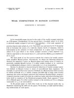
Figure 1: Weighted matchings of Seg
4
and Seg
5
.
where | µ| denotes the number of edges o f µ and EIND(µ) the number of edges {i, i + 1}
with i even. The polynomials U
n
(x, a) came first up in some enumeration problems
in molecular biology [15] and are gene ralized Chebyshev polynomials of the second kind
because we get the classical (monic) Chebyshev polynomials of the second kind [14, p. 2 9]
for a = 1. Recently, Kim and Zeng [7] used (1) and a combinatorial interpretation of

the corresponding moments to evaluate the linearization coefficients of certain products
involving U
n
(x, a), which again generalize and refine results by De Sainte-Catherine and
Viennot [4].
The purpose of this paper consists in studying these matching polynomials yet from
another point of view. We are interested in simultaneous weighted matchings on segment
graphs of different size, and a sk how often the cumulative weight of these matchings, i.e.
the corresponding weighted matching polynomials, can be made equal.
To clarify the problem, we first may take a closer look at a specific example, namely,
at the weighted matching polynomials of Seg
4
and Seg
5
(see Fig. 1):
We see that
U
4
(x, a) = x
4
+ (−1)x
2
+ (−a)x
2
+ (−1)x
2
+ (−1)
2
= x
4

− (a + 2)x
2
+ 1,
U
5
(ˆx, ˆa) = ˆx
5
+ (−1)ˆx
3
+ (−ˆa)ˆx
3
+ (−1)ˆx
3
+ (−ˆa)ˆx
3
+ (−1)
2
ˆx + (−1)(−ˆa)ˆx + (−ˆa)
2
ˆx
= x
5
− 2(ˆa + 1)ˆx
3
+ (ˆa
2
+ ˆa + 1)ˆx.
Given m, n, a and ˆa, how often can we cho ose x and ˆx, such that the cumulative
weights equalize? In other words, regarding our example, how many integral solutions
does U

4
(x, a) = U
5
(ˆx, ˆa) have?
the electronic journal of combinatorics 16 (2009), #R56 2
It is well-known [7, 15] that the family of polynomials {U
n
(x, a)} satisfies a three-term
recurrence equation, i.e.,
U
0
(x, a) = 1, U
1
(x, a) = x, U
n+1
(x, a) = x U
n
(x, a) − λ
n
U
n−1
(x, a), (2)
where λ
2k
= a, λ
2k+1
= 1. Kim and Zeng [7] used Viennot’s theory for orthogonal
polynomials [16, 17] to derive the combinatorial model (1) from (2). Recently, McSor-
ley, Feinsilver and Schott [9] provided a general framework for generating all or t hogonal
polynomials via vertex-matching-partition functions of some suitably labeled paths. The

main point of t he present work is to exhibit a close connection between the enumeration
of a graph-theoretic quantity (i.e., weighted matchings) and a number-theoretic finiteness
result, which here relies on the fact that {U
n
(x, a)} “almost” denotes a classical orthog-
onal polynomial family. Similar diophantine problems evolve from the enumeration of
colored permutations [8] and from lattice point enumeration in polyhedra [1] ( see [12] f or
a list of references). One of the first works studying a diophantine equation which arises
from a combinatorial problem is due to Hajdu [6]; many papers on similar topics have
appeared. In the present graph-theoretic context, however, it is crucial that {U
n
(x, a)}
can be related to classical orthogonal polynomials. Note that by Favard’s theorem [3],
the polynomials U
n
(x, a) given in (2) are orthogonal with respect to a positive-definite
moment functional if and only if a > 0.
Theorem 1.1. Let a, ˆa ∈ Q
+
and m > n ≥ 3. Then the equation
U
m
(x, a) = U
n
(ˆx, ˆa)
has only finitely many integral solutions x, ˆx with the exception of the case
m = 6, n = 3, a = 9/2, ˆa = 59/4, (3)
where x = t, ˆx = t
2
− 4 with t ∈ Z is an infin i te family of solutions. In other words,

besides (3), matchings of segment graphs with sufficiently large node-weights cannot have
equal total matching weigh t.
The paper is organized as follows. We first establish a differential equation of second
order for U
n
(x, a) (Section 2), which may be of independent interest. We then apply
an algorithm due to the first author [13] to characterize all polynomial decompositions
U
n
(x, a) = r(q(x)) with polynomials r, q ∈ R[x] and use a theorem due to Bilu and
Tichy [2] to conclude (Section 3).
2 Differential equation
Recall that the Chebyshev polynomials of the second kind U
n
(x) := U
n
(x, 1) are defined
by
U
0
(x) = 1 , U
1
(x) = 2x, U
n+1
(x) = 2x U
n
(x) − U
n−1
(x). (4)
the electronic journal of combinatorics 16 (2009), #R56 3

Let V
n
(x) = U
n
(x/2) be the monic Chebyshev polynomials of the second kind. In what fol-
lows, we assume that a ∈ R
+
. From (2) we observe that there are polynomials P
n
(x, a) ∈
R[x] and Q
n
(x, a) ∈ R[x] such that U
2n+1
(x, a) = xP
n
(x
2
, a) and U
2n
(x, a) = Q
n
(x
2
, a).
Since
U
n+1
(x, a) = (x
2

− a − 1)U
n−1
(x, a) − a U
n−3
(x, a), n ≥ 3, (5)
by scaling with
W
n
(x, a) = P
n
(
√
ax + a + 1, a)/(
√
a)
n
,
S
n
(x, a) = Q
n
(
√
ax + a + 1, a)/(
√
a)
n
,
we derive from (5) that W
n

(x, a) and S
n
(x, a) satisfy the recurrences:
W
0
(x, a) = 1, W
1
(x, a) = x, W
n+1
(x, a) = xW
n
(x, a) − W
n−1
(x, a),
S
0
(x, a) = 1, S
1
(x, a) = x +
√
a, S
n+1
(x, a) = xS
n
(x, a) − S
n−1
(x, a).
Thus, the polynomials W
n
(x, a) are independent of a and equal the monic Chebyshev

polynomials of the second kind V
n
(x), while the polynomials S
n
(x, a) are co-recursive
versions of the polynomials V
n
(x) (see [5, sec. 2.1 .2 ]). In general, co-recursive orthogonal
polynomials can be easily rewritten in terms of the original non-shifted and the first
associated polynomials (see [5, eq. (20)]). By straightforward calculations we therefore
get the following representation for U
n
(x, a).
Proposition 2.1. We ha ve
U
n
(x, a) =



(
√
a)
k
x V
k

x
2
−a−1

√
a

, n = 2k + 1;
(
√
a)
k

V
k

x
2
−a−1
√
a

+
√
a V
k−1

x
2
−a−1
√
a

, n = 2k.

Taking into account the explicit coefficient formula for Chebyshev polynomials of the
second kind (see e.g. [10]) we obtain
U
n
(x, a) = x
n
+ ε
(n)
2
x
n−2
+ ε
(n)
4
x
n−4
+ ··· ,
where
ε
(n)
2
=

−
1
2
(a + 1)n + a, n even;
−
1
2

(a + 1)(n − 1), n odd,
ε
(n)
4
=

1
8
(n − 2)(n(a + 1)
2
− 4a
2
− 8a), n even;
1
8
(n − 3)(n(a + 1)
2
− a
2
− 6a −1), n odd.
(6)
Similar expressions can be also given for ε
(n)
6
, ε
(n)
8
and ε
(n)
10

(see Appendix). It is
well-known [14] that Chebyshev polynomials of the second kind satisfy a second order
differential equation with polynomial coefficients of degree ≤ 2. With the aid of Proposi-
tion 2.1, it is a direct calculation to come up with a differential equation also for U
n
(x, a)
(however, with polynomial coefficients of higher order).
the electronic journal of combinatorics 16 (2009), #R56 4
Proposition 2.2. Th e polynomials U
n
(x, a) satisfy
A(x) U
n
(x, a) + B(x) U
′
n
(x, a) + C(x) U
′′
n
(x, a) = 0, (7)
where
• n even:
A(x) = −n(n + 1)(n + 2)x
5
+ 3n(n + 2)(a −1)x
3
,
B(x) = 3(n + 1)x
6
− 5(a −1)x

4
− (a − 1) {(3n −1)a − (3n + 7)}x
2
+ (a − 1)
3
,
C(x) = (n + 1)x
7
− {(2n + 3)a + (2n + 1)}x
5
+ (a − 1) {(n + 3)a − (n − 1)}x
3
− (a − 1)
3
x;
• n odd:
A(x) = −n(n + 2)x
4
+ 3(a −1)
2
,
B(x) = 3x
5
− 3(a −1)
2
x,
C(x) = x
6
− 2(a + 1)x
4

+ (a − 1)
2
x
2
.
In the next lemma we make use of the differential equation given in Proposition 2.2.
Lemma 2.3. Let a ∈ R
+
and U
n
(x, a) = r(q(x)) with r, q ∈ R[x] and min(deg r, deg q) ≥
2. Then deg q ≤ 6.
Proof. We use a powerful method due to Sonin, P´olya and Szeg˝o; for more details see [12,
13]. Define the Sonin-type function
h(x) = U
n
(x, a)
2
+
C(x)
A(x)
U
′
n
(x, a)
2
,
which by Proposition 2.2 satisfies h
′
(x) = −

ω (x)
A(x)
2
U
′
n
(x, a)
2
with
ω(x) = (2 B(x) − C
′
(x)) A(x) + C(x)A
′
(x).
If n is even then
ω(x) = x
5

−4n(n + 1)
2
(n + 2)x
6
+ 16 n(n + 1)(n + 2)(a − 1)x
4
+4n(n + 2)(n
2
+ 2n −5)(a −1)
2
x
2

− 8n(n + 2)(a −1)
2
(2an − a − 2n − 5)

.
By Descartes’ rule of signs [10, p. 7] and a ∈ R
+
this polynomial has at most five distinct
real zero es, thus h
′
(x) changes sign at most five times. Since U
n
(x, a) has only simple real
zeroes for a > 0, by Rolle’s theorem so does U
′
n
(x, a). We therefore have deg gcd(U
n
(x, a)−
ζ, U
′
n
(x, a)) ≤ 6, for all ζ ∈ C. Now, suppose a non-trivial decomposition U
n
(x, a) =
r(q(x)) and denote by ζ
0
a zero of r
′
, which exists by deg r ≥ 2. Then both U

n
(x, a)−r(ζ
0
)
and U
′
n
(x, a) are divisible by q(x) − r(ζ
0
). Thus,
deg q ≤ deg(q −ζ) ≤ deg gcd(U
n
(x, a) − ζ, U
′
n
(x, a)) ≤ 6,
which completes the proof for n even. If n is odd then
ω(x) = x

−4n(n + 2)x
8
+ 4(a − 1)
2
n(n + 2)x
4
+ 24(a + 1)(a −1)
2
x
2
− 24(a − 1)

4

,
and a similar arg ument yields the result.
the electronic journal of combinatorics 16 (2009), #R56 5
3 Polynomial decomposi t ion
This section is devoted to a complete characterization of polynomial decompositions of
U
n
(x, a). By a polynomial decomposition of p(x) ∈ R[x] we mean p(x) = r ◦ q(x) with
r, q ∈ R[x] and min(deg r, deg q) ≥ 2. We call two decompositions p = r
1
◦ q
1
= r
2
◦ q
2
equivalent, if there is a linear polynomial κ such that r
2
= r
1
◦ κ and q
2
= κ
−1
◦ q
1
. A
polynomial p is said to be indecomposable, if there is no polynomial decomposition of p.

Lemma 3.1. The generalized Chebyshev polynomials U
n
(x, a) are indecomposable (up to
equivalence) e xcept in the following cases:
(i) n = 2k, k ≥ 2; then U
n
(x, a) = r(x
2
) and r(x) is indecomposable unless (iii).
(ii) n = 6, a =
3
4
; then U
6
(x,
3
4
) = (x
2
− 1) ◦ (x
3
−
9
4
x).
(iii) n = 8, a = 4; then U
8
(x, 4) = (x
2
+ 14 x + 1) ◦(x

4
− 8x
2
).
In view of Lemma 2.3, we have to show that U
n
(x, a) = r(q(x)) with 3 ≤ deg q ≤ 6
leads – in general – to a contradiction. A well-arranged way to equate the (parametric)
coefficients on both sides of the decomposition equation is via the algorithmic approach
(using Gr¨obner techniques) presented in [13, sec. 4]. We shortly recall and outline the
procedure for deg q = 3 and n even, where we find (ii) in Lemma 3.1 . The other cases
are similar (for instance, for deg q = 4 we consider [x
4k− 6
] = [x
4k− 10
] = 0 etc.).
By [12, Proposition 3.3] we can calculate a polynomial ˆq( x) o f degree three from the
data given in (6) which has the following property: If U
n
(x, a) = r(q(x)) with deg q = 3
and q(0) = 0, lcoeff(q(x)) = 1 then necessarily q(x) ≡ ˆq(x). In other words, ˆq(x) is the
only (normed) candidate of degree three. According to [13, Algorithm 1] we here get
ˆq(x) = x
3
−
3k(a + 1) − 2a
2k
x,
such that U
3k

(x, a) = ˆq(x)
k
+ R(x) with R(x) = β
1
x
3k− 4
+ terms of lower order. If there
is a decomposition with a right component of degree three, then necessarily β
1
= 0, which
gives the equation
3k
2
a
2
− 6k
2
a + 3k
2
− 8a
2
k + 4ak + 4a
2
= 0. (8)
Therefore, assuming k > 2, we may suppose that
U
3k
(x, a) = ˆq(x)
k
+ β

2
ˆq(x)
k−2
+ R
1
(x),
where deg R
1
≤ 3k −8. Indeed, the coefficient [x
3k− 8
] in R
1
(x) must be zero. This yields
(k − 2)(162k
5
a
4
+ 162k
5
− 324k
5
a
2
+ 378k
4
a
2
− 189k
4
− 324k

4
a
3
+ 108k
4
a
− 837k
4
a
4
− 72ak
3
+ 72 a
2
k
3
+ 648a
3
k
3
+ 1656a
4
k
3
+ 72 a
2
k
2
− 624a
3

k
2
− 1512a
4
k
2
+ 480a
3
k + 608a
4
k − 8 0a
4
) = 0. (9)
Obviously, k = 2, a = 3/4 is a solution of (8). On the other hand, it is easy to see that
the solutions of (8) and (9) for k ≥ 3 are not admissible (this can b e checked, for instance,
with the help of the Groebner package and the Solve command in MAPLE).
the electronic journal of combinatorics 16 (2009), #R56 6
Corollary 3.2. Let a, ˆa ∈ R
+
and m > n ≥ 3. Then there does not exis t a polynomial
P (x) ∈ R[x] such that
U
m
(x, a) = U
n
(P (x), ˆa) (10)
with the exception of the case
m = 6 , n = 3, a =
9
2

, ˆa =
59
4
, P (x) = x
2
− 4. (11)
Proof. By Lemma 3.1 every decomposition of U
m
(x, a) = r(q(x)) with deg q ≥ 3 implies
deg r ≤ 2, which is not allowed by n ≥ 3. Therefore, we may assume that P (x) = αx
2
+ β
for some α, β ∈ R. First, suppose n ≥ 5. Equating [x
m−2
], [x
m−4
], [x
m−6
], [x
m−8
] and
[x
m−10
] on bo th sides of (10) yields a contradiction (see the Appendix for the corresponding
quantities). It is straightforward to exclude also the case n = 4. Finally, for n = 3 we
have α = 1 a nd the coefficient equations
−3 − 2a = 3β, a
2
+ 2a + 3 = 3β
2

− ˆa − 1, −1 = β
3
− (1 + ˆa)β,
which yield (β, a, ˆa) = (−1, 0, −1) or (β, a, ˆa) = (−4, 9/2 , 59/4). Only the latter solution
is admissible.
As for the final step, we recall the finiteness theorem due to Bilu and Tichy [2]. Again,
for more details we refer to [12]. First some more notation is needed. Let γ, δ ∈ Q \ {0},
r, q, s, t ∈ Z
+
∪ {0} and v(x) ∈ Q[x]. Denote by D
s
(x, a) the Dickson polynomial of the
first kind of degree s defined by
D
0
(x, a) = 2, D
1
(x, a) = x,
D
n+1
(x, a) = xD
n
(x, a) − aD
n−1
(x, a), n ≥ 1,
which satisfies D
n
(x, a) = x
n
+ d

(n)
2
x
n−2
+ d
(n)
4
x
n−4
+ ···, where
d
(n)
2k
=
n
n −k

n − k
k

(−a)
k
. (12)
To state the result, we also need the notion of five types of so-called standard pairs, which
are pairs of polynomials of some sp ecial shape. To begin with, a standard pair of the
first kind is of the type (x
q
, γx
r
v(x)

q
) (or switched), where 0 ≤ r < q, gcd(r, q) = 1 and
r + deg v > 0. A standard pair of the second kind is given by (x
2
, (γx
2
+ δ)v(x)
2
) (or
switched). A standard pair of the third kind is (D
s
(x, γ
t
), D
t
(x, γ
s
)) with s, t ≥ 1 and
gcd(s, t) = 1. A standard pair of the fourth kind is (γ
−s/2
D
s
(x, γ), −δ
−t/2
D
t
(x, δ)) (or
switched) with s, t ≥ 1 and gcd(s, t) = 2. Finally, a standard pair of the fifth kind is of
the form ((γx
2

− 1)
3
, 3x
4
− 4x
3
) (or switched).
The following (less strong) version of the theorem of Bilu and Tichy [2] is sufficient
for our purposes:
the electronic journal of combinatorics 16 (2009), #R56 7
Theorem 3.3 (Bilu/Tichy [2]). Let f(x), g(x) ∈ Q[x] be non-constant polynomia l s and
assume that there do not exist linear polynomials κ
1
, κ
2
∈ Q[x], a polynomial ϕ(x) ∈ Q[x]
and a standard pair (f
1
, g
1
) such that
f = ϕ ◦ f
1
◦ κ
1
and g = ϕ ◦g
1
◦ κ
2
, (13)

then the equation f(x) = g(y) has only fin i tely many integral solutions.
We stress the fact that the proof of Theorem 3.3 is based – b eside other tools – on
Siegel’s theorem on integral points on algebraic curves [11] a nd is therefore ineffective.
This means that we have no upper bound available for the size of solutions x, y. The
standard pairs make up the exceptional cases where one can find an infinite parametric
solution set. According to Theorem 3.3 we here have to check the decomp ositions of
shape (13) whether they match with those given in Lemma 3.1.
To start with, consider the standard pair of the first kind and U
m
(αx + β, a) = ϕ(x
q
).
If q ≥ 3 then β = 0 and ε
(m)
2
α
m−2
= 0, a contradiction. If q = 2 then since m, n ≥ 3 we
have deg ϕ ≥ 2. We distinguish two cases. If deg ϕ = 2 then we are led to the system of
equations
U
4
(α
1
x + β
1
, a) = e
2
x
4

+ e
1
x
2
+ e
0
,
U
6
(α
2
x + β
2
, ˆa) = e
2
x
2
(v
1
x + v
0
)
4
+ e
1
x(v
1
x + v
0
)

2
+ e
0
, (14)
or, respectively, with switched parameters a, ˆa. Equating coefficients on both sides gives
a contradiction.
1
If deg ϕ ≥ 3 then deg(x
r
v(x)
q
) = 1 which by Corollary 3.2 gives m = 6, n = 3, a = 9/2
and ˆa = 59/4. A similar conclusion holds for q = 1.
A standard pair of the second kind is not possible as well. Since m = n, we have
deg v(x) ≥ 1. Ag ain, we distinguish two cases. If deg v(x) ≥ 2 then ϕ(x) is linear, a
contradiction to m, n ≥ 3. On the other hand, if deg v(x) = 1 we have the two equations
(resp. with switched parameters),
U
4
(α
1
x + β
1
, a) = e
2
x
4
+ e
1
x

2
+ e
0
,
U
8
(α
2
x + β
2
, ˆa) = e
2
(γx
2
+ δ)
2
(v
1
x + v
0
)
4
+ e
1
(γx
2
+ δ)(v
1
x + v
0

)
2
+ e
0
. (15)
Again a contradiction arises.
Next, consider the standard pair of the fifth kind and suppose U
m
(αx+β, a) = ϕ((γx
2
−
1)
3
). This implies that ϕ(x) is linear. Again, a contradiction a r ises, since U
′
m
(x, a) o nly
has simple roots whereas the derivative of the right-hand-side polynomial has a triple
root.
It remains to treat the standard pairs of the third and fourth kind. Suppose a stan-
dard pair of the third kind, namely U
m
(α
1
x + β
1
) = ϕ(D
s
(x, γ
t

)) and U
n
(α
2
x + β
2
) =
ϕ(D
t
(x, γ
s
)). By gcd(s, t) = 1 and Lemma 3.1 we see that deg ϕ ≤ 2 (leaving aside the
1
Again, we used safe Groebner computations with MAPLE to conclude for (14) and (15).
the electronic journal of combinatorics 16 (2009), #R56 8
case (11)). First, let ϕ(x) b e linear. Assume m ≥ 7 and U
m
(α
1
x + β
1
) = e
1
D
s
(x, δ) + e
0
with δ = γ
t
. Then using (1 2) the coefficient equations

ε
(m)
2k
= α
2k
1
d
(m)
2k
, k = 1, 2, 3 (16)
yield a contradiction. Therefore,
(m, n) ∈ {(6, 5), (5, 4), (5, 3), (4, 3)}.
Suppose m = 5. Then (16) with k = 1, 2 yields a = (3 ±
√
5)/2 ∈ Q, a contradiction. Let
U
4
(α
1
x + β
1
, a) = e
1
(x
4
− 4 γ
3
x
2
+ 2γ

6
) + e
0
and U
3
(α
2
x + β
2
, ˆa) = e
1
(x
3
− 3 γ
4
x) + e
0
.
This gives e
0
= 0, e
1
= α
4
1
and the contradiction 2α
4
1
γ
6

= 1. Now, suppose ϕ(x) =
e
2
x
2
+ e
1
x + e
0
. By (s, t) = 1 and Lemma 3.1 we have an equation similar to
U
6
(α
1
x + β
1
) = e
2
D
3
(x, δ)
2
+ e
1
D
3
(x, δ) + e
0
,
which directly leads to a contradiction.

Finally, suppose a standard pair of the fourth kind. Again, we conclude deg ϕ ≤ 2.
First, let deg ϕ = 1. Fr om the discussion above we see that (m, n) = (6, 4). Thus,
U
6
(α
1
x + β
1
, a) = e
1

x
6
γ
3
1
−
6x
4
γ
2
1
+
9x
2
γ
1
− 2

+ e

0
,
U
4
(α
2
x + β
2
, ˆa) = e
1

−
x
4
γ
2
2
+
4x
2
γ
2
− 2

+ e
0
.
This gives α
4
2

γ
2
2
= −e
1
and −(2a + 3)α
4
1
γ
2
1
= −6e
1
which implies a < 0, a contradiction.
A similar argument also applies for deg ϕ = 2. This completes the proof of Theorem 1.1.
Remark. It causes no great difficulty to replace the edge weight −1 by −β with β ∈ Q
+
in ( 1) and to conclude in a similar way. Both Proposition 2.2 and Lemma 3 .1 can be
appropriately generalized. As the focus of the paper is on the cross connection between
Diophantine properties and graph quantities, we here omit the details for the general case.
Appen dix
We here append some more upper coefficients of U
n
(x, a) which are needed in the proof
of Corollary 3.2 and in the last section.
ε
(n)
6
=








−
1
48
(n − 4)(3n
2
a + n
2
+ n
2
a
3
+ 3n
2
a
2
− 24na − 2n − 30na
2
−8na
3
+ 72a
2
+ 36a + 12a
3
), n even;

−
1
48
(n − 3)(n − 5)(a + 1)(na
2
− a
2
− 14a + 2na + n − 1), n odd,
the electronic journal of combinatorics 16 (2009), #R56 9
ε
(n)
8
=











1
384
(n − 4)(n −6)(n
2
a
4

+ 4n
2
a
3
+ 6n
2
a
2
+ 4n
2
a + n
2
− 40na − 10na
4
−84na
2
− 2n − 56na
3
+ 64a + 16a
4
+ 288a
2
+ 192a
3
), n even;
1
384
(n − 5)(n −7)(n
2
a

4
+ 4n
2
a
3
+ 6n
2
a
2
+ 4n
2
a + n
2
− 4na
4
− 72na
2
−40na − 4n − 40na
3
+ 84a + 210a
2
+ 3a
4
+ 3 + 84a
3
), n odd.
ε
(n)
10
=
























−
1
3840
(n − 6)(n − 8)(10n
3
a
3

+ n
3
a
5
+ 5n
3
a
4
+ n
3
+ 10n
3
a
2
+ 5n
3
a − 80n
2
a
−110n
2
a
4
− 6n
2
− 220n
2
a
2
− 16n

2
a
5
− 240n
2
a
3
+ 340na
+1520na
2
+ 68na
5
+ 760na
4
+ 8n + 1880na
3
−3200a
2
−400a − 1600a
4
− 4800a
3
− 80a
5
), n even;
−
1
3840
(n − 5)(n − 7)(n − 9)(a + 1)(n
2

a
4
− 4na
4
+ 3a
4
− 56na
3
+ 4n
2
a
3
+132a
3
+ 6n
2
a
2
− 104na
2
+ 498a
2
− 56na + 4n
2
a + 132a
+n
2
− 4n + 3), n odd.
Acknowledgement
The first author is a recipient of an APART-fellowship of the Austrian Academy of Sci-

ences at the University of Waterloo, Canada. Support has also been granted by the Aus-
trian Science Foundation (FWF), project S9604, “Analytic and Probabilistic Methods in
Combinatorics”. The second author is supported by la R´egion Rhˆone-Alpes through the
program “MIRA Recherche 2008”, project 08 034147 01.
References
[1] Y. Bilu, T. Stoll, R.F. Tichy, O ctahedrons with equally many lattice points, Period. Math.
Hungar. 40 (2000), no. 2, 229–238.
[2] Y. Bilu, R.F. Tichy, The Diophantine equation f(x) = g(y), Acta Arith. 95 (2000), 261–288.
[3] T.S. Chihara, An Introduction to Orthogonal Polynomials, Gordon and Breach, New York,
1978.
[4] M. De Sainte-Catherine, X.G. Viennot, Combinatorial Interpretation of Integrals of Prod-
ucts of Hermite, Laguerre and Tchebycheff Polynomials, Lecture Notes in Mathematics,
vol. 1171, Springer-Verlag, 1985, pp. 120–128.
[5] M. Foupouagnigni, W. Koepf, A. Ronveaux, Factorization of forth-order differential equa-
tions for perturbed classical orthogonal polynomials, J. Comput. Appl. Math. 162 (2004),
299–326.
[6] L. Hajdu, On a Diophantine equation concerning the numbe r of integer points in special
domains, Acta Math. Hungar. 78 (1998), 59–70.
[7] D. Kim, J. Zeng, Combinatorics of generalized Tchebycheff polynomials, European J. Com-
bin. 24 (2003), 499–509.
[8] P. Kirschenhofer, O. Pfeiffer, A class of combinatorial Diophantine equations, S´em. Lothar.
Combin. 44 (2000), Art. B44h, 7 pp. (electronic).
the electronic journal of combinatorics 16 (2009), #R56 10
[9] J.P. McSorley, P. Feinsilver, R. Schott, Generating orthogonal polynomials and their deriva-
tives using vertex|matching-partitions of graphs, Ars Combin. 87 (2008), 75–95.
[10] Ze V.V. Prasolov, Polynomials, translated from the 2001 Russian second edition by Dimitry
Leites. Algorithms and Compu tation in Mathematics, S pringer, Berlin, 2004.
[11] C.L. Siegel,
¨
Uber einige Anwendungen Diophantischer Approximationen, Abh. Preuss.

Akad. Wiss. Phys Math. Kl. (1929), no. 1, 209–266.
[12] T. Stoll, Complete decomposition of Di ckson-type recursive polynomials and related Dio-
phantine equations, J. Number Theory, 128 (2008), 1157–1181.
[13] T. Stoll, Decomposition of perturbed Chebyshev polynomials, J. Comp. Appl. Math. 214
(2008), 356–370.
[14] G. Szeg˝o, Orthogonal polynomials, American Mathematical Society C olloquium Publica-
tions, vol. 23, Fourth edition, Providence, R.I., 1975.
[15] M. Vauchassade de Chaumont, X.G. Viennot, Polynˆomes orthogonaux et probl`emes
d’´enum´eration en biologie mol´eculaire, S´em. Lothar. Combin. B081(1984) 8.
[16] X.G. Viennot, Une th´eorie combinatoire des polynˆomes orthogonaux g´en´eraux, Notes de
conf´erences, UQ AM, Montr´eal, 1984.
[17] X.G. Viennot, A combinatorial theory for general orthogonal polynomials with extensions
and applications, Orthogonal polynomials and applications, Lecture Note in Math., 1171,
Springer, Berlin, 1985, pp. 139–157.
the electronic journal of combinatorics 16 (2009), #R56 11