Báo cáo toán học: "Evaluating a Weighted Graph Polynomial for Graphs of Bounded Tree-Width" potx
Bạn đang xem bản rút gọn của tài liệu. Xem và tải ngay bản đầy đủ của tài liệu tại đây (155.68 KB, 14 trang )
Evaluating a Weighted Graph Polynomial for
Graphs of Bounded Tree-Width
S. D. Noble
Department of Mathematical Sciences
Brunel University
Kingston Lane, Uxbridge
UB8 3PH, U.K.
Submitted: Oct 30, 2006; Accepted: May 18, 2009; Published: May 29, 2009
Mathematics S ubject Classification: 05C85, 05C15, 68R10
Abstract
We show that for any k there is a polynomial time algorithm to evaluate the
weighted graph p olynomial U of any graph with tree-width at most k at any point.
For a graph with n vertices, the algorithm requires O(a
k
n
2k+ 3
) arithm etical opera-
tions, where a
k
depends only on k.
1 Introduction
Motivated by a series of papers [9, 10, 1 1], the weighted graph polynomial U was intro-
duced in [22]. Chmutov, Duzhin and Lando [9, 10, 11] introduce a graph polynomial
derived from Vassiliev invariants of knots and note that this polynomial does not include
the Tutte polynomial as a special case. With a slight generalisation of their definition we
obtain the weighted graph polynomial U that does include the Tutte polynomial.
The attraction of U is that it contains many other graph invariants as specialisations,
for instance the 2 -polymatroid rank generating function of O xley and Whittle [23], and as
a consequence the matching polynomial, the stable set polynomial [13] and the symmetric
function generalisation of the chromatic polynomial [27]. Note however that there are
non-isomorphic graphs with the same U polynomial. This is a corolla ry of a result of
Sarmiento [26], showing that the coefficients of U and the polychromate determine one
another. It remains an open problem to determine whether or not there are two non-
isomorphic trees with the same U polynomial. We introduce U in Section 2 and review
some of these results in more detail.
The notion of tree-width was introduced by Robertson and Seymour as a key tool in
their work on the graph minors project [24, 25]. An equivalent notion, studied extensively
by Arnborg and Proskurowski, (see for instance [3, 4]), is that of a partial k-tree.
the electronic journal of combinatorics 16 (2009), #R64 1
Many well-studied classes of graphs have bo unded tree-width: for instance, series-
parallel networks are the graphs with tree-width at most two. A large class of g r aph
problems, which are thought to be intractable, can be solved when the input is restricted
to graphs with tree-width at most a fixed constant k. For example, the NP-complete
problems, 3-Colouring and Hamiltonian Circuit can be solved in linear time for graphs of
bounded tree-width [4]. For a g ood survey of tree-width see [5].
When the underlying graph is obvious, we let n be its number of vertices, m be its
number of edges and p be the largest size of a set of mutually parallel edges.
Theorem 1.1. For any k ∈ N, there exists an algorithm A
k
with the following prop-
erties. The input is any graph G, with tree-width at most k, and rationals x
1
=
p
1
/q
1
, . . . , x
n
= p
n
/q
n
and y = p
0
/q
0
such that for all i, p
i
and q
i
are coprime. The
output is U
G
(x
1
, . . . , x
n
, y); the running time is
O(a
k
n
2k+ 3
(n
2
+ m)r log p log(r(n + m)) log(log(r(n + m)))),
where r = log(max{|p
0
|, . . . , |p
n
|, |q
0
|, . . . , |q
n
|}) and a
k
depends only on k.
The result extends that of [2 0] and independently [2] where an algorithm to evaluate
the Tutte p olynomial of a graph having tree-width at most k is presented. In [20], the
algorithm given requires only a linear (in n) number of multiplications. Despite using the
same basic idea as in [20], we are unable to reduce the amount of computational effort
required to evaluate U down to O(n
α
) operations, where α is independent of k.
More recently Hlinˇen´y [15] has shown that the Tutte polynomial is computable in
polynomial time when the input is restricted to matroids with bounded branchwidth rep-
resentable over a finite field. Furthermore Makowsky [17] and Makowsky and Mari˜no [19]
have shown that there are polynomial time alg orithms to evaluate a wide range of graph
polynomials that are definable in monadic second order logic when the input graph has
bounded tree-width. Examples include the Tutte polynomial for coloured graphs due to
Bollob´as and Riordan [7] and certain instances of the very general graph polynomials
introduced by Farrell [14]. However it has been shown that U is not even definable in
second order logic [18], so none of these results applies. For a recent survey covering the
complexity of evaluating many of these polynomials, see [21].
2 A weighted graph polynomial
We begin with a few definitions and then define U, the weighted graph polynomial. We
then state some of the key results about U for which the proofs may be found in [22 ].
Most of our definitions are standard. Our graphs are allowed to have loops and multiple
edges. By a simple graph we mean one with no loops or multiple edges. If G is a graph
and A ⊆ E(G) then G|A is the graph with vertex set V (G) and edge set A. However,
in general, our subgraphs do not have to be spanning, that is if H is a subgraph of G
then we do not require that V (H) = V (G). The number of connected components of a
the electronic journal of combinatorics 16 (2009), #R64 2
graph G is denoted by k(G). The rank of a set A ⊆ E is denoted by r(A) and defined by
r(A) = |V (G)| − k(G|A).
The original definition of U involved a recurrence relation using deletion and contrac-
tion, but for the purposes of this paper it is more useful to define U using the “states
model expansion” from Proposition 5.1 in [22].
U
G
(x, y) =
A⊆E
x
n
1
x
n
2
· · · x
n
k(G|A)
(y − 1)
|A|−r(A)
, (2.1)
where n
1
, . . . , n
k(G|A)
are the numbers of vertices in the connected compo nents of G|A.
For example, if G is a triangle then
U
G
(x, y) = x
3
1
+ 3x
1
x
2
+ 2x
3
+ yx
3
.
We now state some of the results from [22] concerning specialisations of U. The Tutte
polynomial T
G
(x, y) is an extremely well-studied two-variable graph polynomial which is
defined as follows:
T
G
(x, y) =
A⊆E
(x − 1)
r(E)−r(A)
(y − 1)
|A|−r(A)
.
Evaluations of T include the number of spanning trees, number of spanning forests, the
chromatic polynomial and the reliability polynomial as well as applications in statistical
mechanics and knot theory. See for instance [8, 29].
Proposition 2.1. For any graph G,
T
G
(x, y) = (x − 1)
−k(G)
U
G
(x
i
= x − 1, y).
Note that we have abused notation somewhat by writing U
G
(x
i
= x − 1, y) where we
mean for all i setting x
i
= x − 1. It is well-known that if the class of input graphs is not
restricted, then apart from along one specific curve and at a small number of other specific
points, it is #P -hard to evaluate the Tutte polynomial [16]. Except for the addition of one
extra exceptional curve this result may be extended to bipartite planar graphs [28]. These
results combined with Proposition 2.1 show that if we do not restrict the class of input
graphs then the problem of eva luating U at a point specified in the input is #P -hard.
The 2-polymatroid ra nk generating function S
G
(u, v) was introduced by Oxley and
Whittle in [23] and is defined as follows. Given a graph G = (V, E) and A ⊆ E let f(A)
denote the number of vertices of G that are an endpoint of an edge in A. Then
S
G
(u, v) =
A⊆E
u
|V (G)|−f (A)
v
2|A|−f (A)
.
S contains the matching polynomial as a specialisation.
Proposition 2.2. Let G be a loopless graph with no isolated vertices. Then
S
G
(u, v) = U
G
(x
1
= u, x
2
= 1, x
j
= v
j−2
for j > 2, y = v
2
+ 1).
the electronic journal of combinatorics 16 (2009), #R64 3
A stable set in a graph G = (V, E) is a set S o f vertices fo r which G has no edge with
both endpoints in S. The stability polynomial A
G
(p) was introduced by Farr in [13] and
is given by
A
G
(p) =
U∈S(G)
p
|U |
(1 − p)
|V \U|
,
where S(G) is the set o f all stable sets of G.
Proposition 2.3. If G is loopless then A(G; p) is given by
A(G; p) = U
G
(x
1
= 1, x
j
= −(−p)
j
for j ≥ 2, y = 0).
The symmetric function generalisation of the chromatic polynomial was developed
by Stanley in [27]. Let G be a graph with vertex set V = {v
1
, . . . , v
n
}. Then X
G
is a
homogeneous symmetric function of degree n defined by
X
G
(x
1
, x
2
, . . .) =
χ
x
χ(v
1
)
x
χ(v
2
)
· · · x
χ(v
n
)
where the sum ranges over all proper colourings χ : V → Z
+
. Let p
0
= 1 and for r ≥ 1
let
p
r
(x
1
, x
2
, . . .) =
∞
i=1
x
r
i
.
Then we have the following.
Proposition 2.4. For any graph G,
X
G
(x
1
, x
2
, . . .) = (−1)
|V |
U
G
(x
j
= −p
j
, y = 0).
3 Preliminary results
We begin this section with a f ew definitions that are needed in the algorithm. Although
the ideas behind the algorithm are quite simple, they do involve introducing a lot of
notation. A weighted partition of a set A consists of a partition π of A into non-empty
blocks, together with the assignment to each block of a non-negative integer label. If B
is a block in a weighted partition π, we write B ∈ π and we denote the label of B by
w
π
(B). The number of blocks in π is denoted by #π.
Given two weighted partitions π
1
and π
2
, of the same set, we define their join π =
π
1
∨ π
2
as follows. The blocks are minimal sets such that if two elements ar e in the same
block of either π
1
or π
2
then they are in the same block of π. In other words, before
considering weights, the join operation corresponds to join in the partition lattice. If B
is a block of π then for i = 1, 2, B is t he disjoint union of a collection of blocks from π
i
.
We define w
π
(B) by
w
π
(B) =
B
′
∈π
1
:
B
′
⊆B
w
π
1
(B
′
) +
B
′
∈π
2
:
B
′
⊆B
w
π
2
(B
′
).
the electronic journal of combinatorics 16 (2009), #R64 4
Let G = (V, E) be a graph and A ⊆ E. Let π(A) be the partition of V given by the
connected components of G|A. We use π(A) to make two definitions. The first definition
is the weighted partition induced by A on S and we denote it by π
G
(S, A), often omitting
G when it is obvious fro m the context. The weighted partition π
G
(S, A) is formed from
π(A) by labelling each block B with |B−S| and deleting all the elements of V −S together
with any empty blocks that are created in the deletion process.
Now let c(S, A, i) denote the number of blocks of π(A) contained entirely in S and
having i vertices. The component type of A on S is the monomial
x(S, A) =
∞
i=1
x
c(S,A,i)
i
.
Finally we let c(S, A) =
n
i=1
c(S, A, i).
Let G be the graph in Figure 1, let S = {v
1
, v
2
, v
4
, v
8
} and A = {e, f, g, h}. Then π(A)
has blocks {v
1
, v
2
, v
4
, v
7
}, {v
3
, v
5
}, {v
6
}, {v
8
}. So π
G
(S, A) has blocks {v
1
, v
2
, v
4
} and {v
8
}
with weights one and zero respectively. Furthermore x(V − S, A) = x
1
x
2
corresponding
to the blo cks {v
3
, v
5
} and {v
6
}.
v
2
v
3
v
1
v
4
v
5
v
6
v
7
v
8
e
f
g
h
Figure 1: Weighted partition example
Note that
U
G
(x, y) =
A⊆E
x(V, A)(y − 1)
|A|−r(A)
and also for any S ⊆ V
U
G
(x, y) =
A⊆E
x(V − S, A)
B∈π(S,A)
x
w
π
(B)+|B|
(y − 1)
|A|−r(A)
. (3.1)
For G = (V, E) and S ⊆ V , let Π(S) be the set of all weighted partitions of S such
that the sum of the weights is at most n. Note that |Π(S)| ≤ n
|S|
B(|S|) where B(k)
denotes the kth Bell Number. Let Π
0
(S) denote the set of all weighted partitions o f S
with each block having weight zero.
In the algorithm we compute the evaluation of several polynomials which resemble the
states model expansion of U (2.1), except that we restrict the summation to those sets of
edges inducing a particular weighted partition.
the electronic journal of combinatorics 16 (2009), #R64 5
Let G = (V, E) and S ⊆ V . Let π be a weighted partition of S. Then we define
U
S
G
(π; x, y) =
A⊆E:
π
G
(S,A)=π
x(V − S, A)(y − 1)
|A|−r(A)
. (3.2)
In order to be completely clear, x and y will be specified in the input so we will think
of U
S
G
as an evaluation of a polynomial rather than a polynomial.
In Section 5, we shall see that the algorithm works by building up the set of pairs
U(H, S) = {(π, U
S
H
(π; x, y)) : π ∈ Π(S), U
S
H
(π; x, y) = 0},
for successively larger subgraphs H of G and certain sets S ⊆ V (H). The key step occurs
when G is the union o f two edge-disjoint graphs G
1
and G
2
such that V (G
1
)∩V (G
2
) = S.
Then the following lemma shows that U(G, S) may be computed from U(G
1
, S) and
U(G
2
, S).
Lemma 3.1. Let G
1
= (V
1
, E
1
), G
2
= (V
2
, E
2
) be graphs having disjoint edge sets. Let
S = V
1
∩ V
2
and let G = G
1
∪ G
2
. Then for all π ∈ Π(S),
U
S
G
(π; x, y) =
U
S
G
1
(π
1
; x, y)U
S
G
2
(π
2
; x, y)(y − 1)
(#π+|S|−#π
1
−#π
2
)
,
where the summation is over all π
1
, π
2
∈ Π(S) such that π
1
∨ π
2
= π.
Proof. Let V = V
1
∪ V
2
and E = E
1
∪ E
2
. Recall that the definition of U
S
G
is as follows.
U
S
G
(π; x, y) =
A⊆E:
π(S,A)=π
x(V − S, A)(y − 1)
|A|−r(A)
.
Now let A
1
⊆ E
1
, A
2
⊆ E
2
and let A = A
1
∪ A
2
. We claim that π
G
(S, A) = π
G
1
(S, A
1
) ∨
π
G
2
(S, A
2
). Suppose the weighted partitions induced on S by A
1
, A
2
and A are π
1
, π
2
and π respectively. Two vertices in the same block of either π
1
or π
2
must be in t he
same block of π. Hence the blocks of π are the blocks of π
1
∨ π
2
. Let B be a block of
π and for i = 1, 2 let w
i
(B) denote the number of vertices of V
i
− S that lie on a path
beginning at a vertex in B and containing only edges of A
i
. Then the label on B in π is
w
1
(B) + w
2
(B). Now B is the disjoint union of blocks of π
1
. It is not difficult to see that
the sum of the lab els on these blocks is w
1
(B) and a similar result holds considering π
2
.
Hence π = π
1
∨ π
2
as required. Now π
G
(S, A
1
) = π
G
1
(S, A
1
) and π
G
(S, A
2
) = π
G
2
(S, A
2
),
so we have
A⊆E:
π
G
(S,A)=π
x(V − S, A)(y − 1)
|A|−r(A)
=
π
1
,π
2
:
π
1
∨π
2
=π
A
1
⊆E
1
:
π
G
1
(S,A
1
)=π
1
A
2
⊆E
2
:
π
G
2
(S,A
2
)=π
2
x(V − S, A
1
∪ A
2
)(y − 1)
|A
1
|+|A
2
|−r(A
1
∪A
2
)
.
the electronic journal of combinatorics 16 (2009), #R64 6
Edges of G
1
do not have either endpoint in V
2
− S and similarly edges of G
2
do not
have either endpoint in V
1
− S. Consequently if A
1
⊆ E
1
and A
2
⊆ E
2
then for a ll i,
c(V − S, A
1
∪ A
2
, i) = c(V
1
− S, A
1
, i) + c(V
2
− S, A
2
, i) which implies that
x(V − S, A
1
∪ A
2
) = x(V
1
− S, A
1
)x(V
2
− S, A
2
).
Furthermore for i = 1, 2 we have
r(A
i
) = |V
i
| − c(V
i
− S, A
i
) − #π(S, A
i
)
and similarly
r(A) = |V | − c(V − S, A) − #π(S, A).
So
r(A) = |V | − c(V − S, A) − #π(S, A)
= |V
1
| − c(V
1
− S, A
1
) − #π(S, A
1
)
+ |V
2
| − c(V
2
− S, A
2
) − #π(S, A
2
)
+ (#π(S, A
1
) + #π(S, A
2
) − #π(S, A) − |S|)
= r(A
1
) + r(A
2
) + #π(S, A
1
) + #π(S, A
2
) − #π(S, A) − |S|.
Finally we get
π
1
,π
2
:
π
1
∨π
2
=π
A
1
⊆E
1
:
π
G
1
(S,A
1
)=π
1
A
2
⊆E
2
:
π
G
2
(S,A
2
)=π
2
x(V − S, A
1
∪ A
2
)(y − 1)
|A
1
|+|A
2
|−r(A
1
∪A
2
)
=
π
1
,π
2
:
π
1
∨π
2
=π
A
1
⊆E
1
:
π
G
1
(S,A
1
)=π
1
A
2
⊆E
2
:
π
G
2
(S,A
2
)=π
2
x(V
1
− S, A
1
)(y − 1)
|A
1
|−r(A
1
)
· x(V
2
− S, A
2
)(y − 1)
|A
2
|−r(A
2
)
(y − 1)
(#π+|S|−#π
1
−#π
2
)
=
π
1
,π
2
:
π
1
∨π
2
=π
U
S
G
1
(π
1
; x, y)U
S
G
2
(π
2
; x, y)(y − 1)
(#π+|S|−#π
1
−#π
2
)
,
as required.
4 Tree-width
We begin with definitions of tree-decompositions and of tree-width. A tree-decomposition
of a graph G = (V, E) is a pair
S = {S
i
|i ∈ I}, T = (I, F)
where S is a family of subsets
of V , one for each vertex of T , and T is a tr ee such that
•
i∈I
S
i
= V .
• for all edges {v, w} ∈ E, there exists i ∈ I such that {v, w} ⊆ S
i
.
• for all i, j, k ∈ I, if j is on the path from i to k in T , then S
i
∩ S
k
⊆ S
j
.
the electronic journal of combinatorics 16 (2009), #R64 7
The width of a tree-decomposition is max
i∈I
|S
i
| − 1. The tree-width of a g r aph G is
the minimum width of a tree-decomposition of G.
Given a simple graph with tree-width at most k, the algorithm given in [6] will, in
time O(g(k)n), produce a tree-decomposition of width at most k. Note however that
g(k) = k
5
(2k + 1)
2k− 1
((4k + 5)
4k+ 5
(2
2k+ 5
/3)
4k+ 5
)
4k+ 1
.
Let T
′
= (S
′
, T
′
) be the output of the algor ithm. Suppose we arbitrarily give T
′
a root
r. Then it is easy to modify T
′
to produce a tree-decomposition T =
{S
i
|i ∈ I}, T =
(I, F)
satisfying the following properties.
1. T is rooted.
2. For all i ∈ I, |S
i
| = k + 1.
3. If S
i
and S
j
are joined by an edge of T then |S
i
∩ S
j
| ≥ k.
4. For all i ∈ I, there is a leaf l of T such that S
l
= S
i
.
5. For all i ∈ I, either i is a leaf of T or i has two children.
6. |I| ≤ 2n.
This f ollows using an easy induction and the procedure may be carried out in time
O(g(k)n). We call such a tree-decomposition, a reduced rooted tree-decomposition.
5 The algorithm
We now describe how the algorithm works and discuss its complexity. Let k be a fixed
strictly positive integer. We assume that we are given a graph G with tree-width at most
k, and rationals x
1
, . . . , x
n
and y. Remove all but one edge from each parallel class to
give G
′
. Define m : E(G
′
) → Z
+
so that m(e) is the size of the parallel class (that is the
maximal set of mutually parallel edges) containing e in G. Compute a reduced rooted
tree-decomposition (S, T ) of G
′
with width at most k.
Using pro perty (4) of a reduced rooted tree-decomposition, we see that we may arbi-
trarily associate each edge e = {u, v} of G
′
with a leaf l of T such that {u, v} ⊆ S
l
. Let E
l
denote the set of edges associated with leaf l. Then the collection {E
l
: l is a leaf of T }
forms a partition of E(G
′
).
Removing multiple edges and loops from G and defining m(e) requires time O(m).
Computing a tree-decomposition using the algorithm in [6] requires time O(g(k)n) and
producing a reduced tree-decomposition fro m this requires time O(g(k)n). Finally com-
puting the partition {E
l
: l is a leaf of T } needs time O(k
2
n).
For i, j ∈ I, we write i j if i = j or i is a descendant of j in T . Now for each
i ∈ I, let G
i
denote the subgraph of G for which the vertex set is
ji
S
j
and the edge
set consists of all edges of G for which the corresp onding edge of G
′
is in E
l
for some l
the electronic journal of combinatorics 16 (2009), #R64 8
that is a descendant i in T. (It is not necessary for the algorithm to explicitly compute
or construct any of these subgraphs.)
Then for each i ∈ V (T) the algorithm iteratively computes the set of pairs
U(G
i
, S
i
) = { ( π, U
S
i
G
i
(π; x, y)) : π ∈ Π(S
i
), U
S
i
G
i
(π; x, y) = 0},
by working upwards through the tree computing U(G
i
, S
i
) only when the sets corre-
sponding to each of its descendants have been computed. Let β(n, m, k, x, y) denote
the maximum time needed for one multiplication or addition during the computation of
U
G
(x, y).
We first deal with the computation at leaves of T .
Lemma 5.1. If l is a leaf, then U(G
l
, S
l
) can be computed in time O(2
(k+1)
2
k
2
log(p)β).
Proof. Since V (G
l
) = S
l
, U
S
l
G
l
(π; x) = 0 unless the weight o f each block of π is zero. So
we may restrict our attention to weighted partitions where each block has weight zero. If
π ∈ Π
0
(S
i
) and y = 1 then
U
S
l
G
l
(π; x) =
A⊆E
l
:π(S
l
,A)=π
(y − 1)
−r(A)
e∈A
(y
m(e)
− 1).
If π ∈ Π
0
(S
l
) and y = 1 then
U
S
l
G
l
(π; x) =
A⊆E
l
:r(A)=|A|
π(S
l
,A)=π
e∈A
m(e).
We compute all these sums in parallel by making one pass through all A ⊆ E
l
, determining
π(S
l
, A) in time O(k
2
), computing (y − 1)
−r(A)
e∈A
(y
m(e)
− 1) or
e∈A
m(e) in time
k
2
log(p)β and adding the result on to the appropriate sum.
The next two lemmas deal with the computation at vertices of T that are not leaves.
Suppose that j is the child of i in T . Recall that S
i
\ S
j
contains at most one vertex.
Define G
+
j
as follows: if S
i
= S
j
then let G
+
j
= G
j
and otherwise form G
+
j
from G
j
by
adding the unique vertex of S
i
\ S
j
as an isolated vertex.
First we show how to compute U(G
+
j
, S
i
) from U(G
j
, S
j
). This is really a bookkeeping
exercise but its description is slightly complicated. If S
i
= S
j
then there is nothing
to be done. Otherwise let S
j
\ S
i
= {s} and S
i
\ S
j
= {t}. Let A ⊆ E(G
j
) and let
π = π
G
j
(S
j
, A). Suppose the block of π containing s is B . Now there are two cases to
consider. If B = {s} then π
G
+
j
(S
i
, A) is formed from π
G
j
(S
j
, A) by adding {t} as a block
with weight zero, deleting s from B and incrementing the weight of B by one. Furthermore
x(V (G
+
j
) \ S
i
, A) = x(V (G
j
) \ S
j
, A). On the other hand if B = {s} then π
G
+
j
(S
i
, A) is
formed from π
G
j
(S
j
, A) by adding {t} as a block with weight zero a nd deleting B. Now
x(V (G
+
j
) \ S
i
, A) = x(V (G
j
) \ S
j
, A)x
w(B)+1
. Notice that in either case π
G
+
j
(S
i
, A) and
x(V (G
+
j
)\S
i
, A) depend on A only via π
G
j
(S
j
, A) and x(V (G
j
)\S
j
, A). Consequently for
the electronic journal of combinatorics 16 (2009), #R64 9
any π ∈ Π(S) we define π
t
s
by adding {t} as a block with weight zero and then proceeding
as follows. If {s} is a block o f π then delete it, otherwise increment the weight of the
block containing s by one and then delete s. If B is the block of π containing s then we
define
x(s, π) =
x
w(B)+1
if B = {s},
1 otherwise.
Lemma 5.2. Let j be a child of i in T with S
i
= S
j
and let π
0
∈ Π(S
i
). Then using the
notation above
U
S
i
G
+
j
(π
0
; x, y) =
π∈Π(S
j
):π
t
s
=π
0
U
S
j
G
j
(π; x, y)x(s, π).
Furthermore U(G
+
j
, S
i
) can be computed from U(G
j
, S
j
) in time O(B(k)n
k+1
β).
Proof. First note tha t if {t} is not a block o f π
0
then U
S
i
G
+
j
(π
0
; x, y) = 0. Otherwise by (3.2)
we have
U
S
i
G
+
j
(π
0
; x, y) =
A⊆E(G
+
j
):
π(S
i
,A)=π
0
x(V (G
+
j
) \ S
i
, A)(y − 1)
|A|−r(A)
. (5.1)
Furthermore we have
π∈Π(S
j
):π
t
s
=π
0
U
S
j
G
j
(π; x, y)x(s, π)
=
π∈Π(S
j
):
π
t
s
=π
0
A⊆E(G
j
):
π(S
j
,A)=π
x(V (G
j
) \ S
j
, A)(y − 1)
|A|−r(A)
x(s, π). (5.2)
From the discussion preceding the lemma and the fact that E(G
j
) = E(G
+
j
), a set
A contributes to the sum in (5.1) if and only if it contributes to the right-hand side
of (5.2). Furthermore fo r such a set A, the discussion preceding the lemma implies that
x(V (G
+
j
) \ S
i
, A) = x(V (G
j
) \ S
j
, A)x(s, π). Hence the first par t of the lemma follows.
To see that the complexity calculation is correct first recall that |Π(S
i
)| = n
k+1
B(k+1).
However if t does not occur as a singleton block of weight zero in π
0
then U
S
i
G
+
j
(π
0
; x, y) = 0,
so we only have to compute U
S
i
G
+
j
(π
0
; x, y) for n
k
B(k) different weighted partitions π
0
.
For such a weighted partition π
0
, we must determine which weighted partitions of S
j
appear in the sum in (5.1). There are two types, those in which s appears as a singleton
block and t hose in which s does not. In the former case we may add s to π
0
as a singleton
block with any of the possible O(n) weights and in the latter case we may add s to any
of the at most k blocks of π
0
. In both cases we remove the singleton block containing t.
It remains to calculate x(s, π) for each of these O(n) partitions and finally compute the
sum. The total time required is O(B(k)n
k+1
β) as required.
The second lemma follows from Lemma 3.1.
the electronic journal of combinatorics 16 (2009), #R64 10
Lemma 5.3. Let j and k be the children of i in T . Then U(G
i
, S
i
) can be computed from
U(G
+
j
, S
i
) and U(G
+
k
, S
i
) in time O((B(k + 1))
2
kn
2k+ 2
(k + β)).
Proof. Applying Lemma 3.1 we see that For all π ∈ Π(S
i
),
U
S
i
G
i
(π; x, y) =
U
S
i
G
+
j
(π
1
; x, y)U
S
i
G
+
k
(π
2
; x, y)(y − 1)
(#π+k+1−#π
1
−#π
2
)
,
where the summation is over all π
1
, π
2
∈ Π(S) such that π
1
∨ π
2
= π.
We can compute U(G
i
, S
i
) by making one pass through all pairs (π
1
, U
S
i
G
+
j
(π
1
; x, y))
and (π
2
, U
S
i
G
+
k
(π
2
; x, y)) of elements from U(G
+
j
, S
i
) and U(G
+
k
, S
i
) respectively, computing
π
1
∨ π
2
and adding the contribution from this pair to the sum giving (π
1
∨ π
2
, U
S
i
G
i
(π
1
∨
π
2
; x, y)). To find π
1
∨π
2
requires time O(k
2
+kβ); to find (y −1)
(#π+|S|−#π
1
−#π
2
)
requires
time O(kβ). Consequently the complexity estimate follows.
Together, the preceding two lemmas show that for any i ∈ I with children j and k,
we can calculate U(G
i
, S
i
) from U(G
j
, S
j
) and U(G
k
, S
k
). Finally we can recover U
G
(x, y)
given U(G
r
, S
r
), where r is the root of T .
Lemma 5.4. Let r be the root of T . Then
U
G
(x, y) =
π∈Π(S
r
)
U
S
r
G
r
(π; x, y)
B∈π
x
(w
π
(B)+|B|)
.
Furthermore U
G
(x, y) can be computed from U(G
r
, S
r
) in time O(B(k + 1)n
k+1
kβ).
Proof. By applying the definition of U
S
G
and the fact that G
r
= G, we have
π∈Π(S
r
)
U
S
r
G
r
(π; x, y)
B∈π
x
(w
π
(B)+|B|)
=
A⊆E(G)
x(V − S
r
, A)(y − 1)
|A|−r(A)
B∈π(S
r
,A)
x
(w
π(S
r
,A)
(B)+|B|)
.
Comparing this expression with (3.1), we see that this is exactly U
G
. The sum contains
O(B(k + 1)n
k+1
) terms and to compute each term requires time O(kβ), so the complexity
calculation is correct.
By combining Lemmas 5.1–5.4 and the remarks at the beginning of this section, we
see that the overall running time of the algorithm is O(g(k)n
2k+ 3
log(p)β). Finally we
compute bounds on the numbers involved in the computations. When y = 1 the numbers
involved other than the weights of the blocks of partitions may be written in the following
form:
A∈A
x
a
1
1
· · · x
a
n
n
(y − 1)
|A|−r(A)
the electronic journal of combinatorics 16 (2009), #R64 11
where A is a collection of subsets of E(G) and
n
i=1
a
i
≤ n. Recall that for a ll i, x
i
= p
i
/q
i
and y = p
0
/q
0
. Let
M = max{|p
0
|, |p
1
|, . . . , |p
n
|, |q
0
|, |q
1
|, . . . , |q
n
|}.
Then
A∈A
x
a
1
1
· · · x
a
n
n
(y − 1)
|A|−r(A)
=
A∈A
p
a
1
1
. . . p
a
n
n
(p
0
− q
0
)
|A|−r(A)
q
a
1
1
. . . q
a
n
n
q
|A|−r(A)
0
=
A∈A
p
a
1
1
q
n−a
1
1
. . . p
a
n
n
q
n−a
n
n
(p
0
− q
0
)
|A|−r(A)
q
m+r(A)−|A|
0
q
n
1
. . . q
n
n
q
m
0
.
Considering the denominator, we have |q
n
1
. . . q
n
n
q
m
0
| ≤ M
n
2
+m
. For the numerator we have
A⊆E(G)
p
a
1
1
q
n−a
1
1
. . . p
a
n
n
q
n−a
n
n
(p
0
− q
0
)
|A|−r(A)
q
m+r(A)−|A|
0
≤ 2
m
M
n
2
(2M)
m
.
Similar bounds hold when y = 1. Hence a bound on the size of any of the numbers
occurring in the algorithm is M
n
2
+m
4
m
. To add, subtract, multiply or divide two b-bit
integers takes at most O(b log(b) log(log(b))) time [1, 12]. So the overall running time of
the algorithm is
O(g(k)n
2k+ 3
(n
2
+ m) log(p)r log(r(n + m)) log(log(r(n + m)))),
where r = log(max{|p
0
|, . . . , |p
n
|, |q
0
|, . . . , |q
n
|}).
When the graph is simple, m ≤ kn a nd so the running time is at most
O(g(k)n
2k+ 5
r log(rn) log(log(rn))).
Acknowledgement
We thank Janos Makowsky and the anonymous referee for their helpful comments.
References
[1] A. V. Aho, J. E. Hopcroft, and J. D. Ullman. The Design and Analysis of Computer
Algorithms. Addison-Wesley, Reading Massachusetts, 1974.
[2] A. Andrzejak. A polynomial-time algorithm for computation of the Tutte polynomi-
als of graphs of bounded treewidth. Discrete Mathematics, 190:39–54, 1998.
[3] S. Arnborg, D. G. Corneil, and A. Proskurowski. Complexity of finding embeddings
in a k-tree. SIAM Journal of Algebraic and Discrete Methods, 8:277–284, 1987 .
the electronic journal of combinatorics 16 (2009), #R64 12
[4] S. Arnborg and A. Proskurowski. Linear time algorithms for NP-hard problems
restricted to pa rt ia l k-trees. Discrete Applied Mathematics, 23:1 1–24, 1989.
[5] H. L. Bodlaender. A tourist guide through treewidth. Acta Cybernetica, 11:1–21,
1993.
[6] H. L. Bodlaender. A linear time algorithm for finding tree-decompositions of small
treewidth. SIAM Journal on Computing, 25:1305–1317, 1996.
[7] B. Bollob´as and O. Riordan. A Tutte polynomial for coloured graphs. Combinatorics,
Probability and Computing, 8:45–94, 1999.
[8] T. H. Brylawski and J. G. Oxley. The Tutte polynomial and its applications. In
N. White, editor, Matroid applications, pages 12 3–225. Cambridge University Press,
Cambridge, 1992.
[9] S. V. Chmutov, S. V. Duzhin, and S. K. Lando. Vassiliev knot invariants: I. Intro-
duction. Advances in Soviet Mathematics, 21 :1 17–126, 1994.
[10] S. V. Chmutov, S. V. Duzhin, and S. K. Lando. Vassiliev knot invariants: II. Inter-
section graph for trees. Advances in Soviet Mathematics, 21:127–134, 1994.
[11] S. V. Chmutov, S. V. Duzhin, a nd S. K. Lando. Vassiliev knot invariants: III. Forest
algebra and weighted graphs. Advances in Soviet Mathematics, 21:135–145, 1994.
[12] J. Edmonds. Systems of distinct representatives and linear algebra. Journal of
Research of the National Bureau of Standards Section B, 71B:241–2 45, 1967.
[13] G. E. Farr. A correlation inequality involving stable sets and chromatic polynomials.
Journal of Combinatorial Theory Series B, 58:14–21, 1993.
[14] E. J. Farrell. On a general class of graph polynomials. Journal of Combinatorial
Theory Series B, 2 6:111–122, 1979.
[15] P. Hlinˇen´y. The Tutte polynomial for matroids of bounded branch-width. Combina-
torics, Probability and Computing, 15:397–409, 2006.
[16] F. Jaeger, D. L. Vertigan, and D. J. A. Welsh. On the computational complexity
of the Jones a nd Tutte polynomials. Mathematical Proceedings of the Cambridge
Philosophical Society, 108:35 –53, 1990.
[17] J. A. Makowsky. Coloured Tutte polynomials and Kaufmann brackets f or graphs of
bounded tree width. Discrete Applied Mathematics, 145:276 –290, 2005.
[18] J. A. Makowsky. Personal Communication, 2008.
[19] J. A. Makowsky and J. P. Mari˜no. Farrell p olynomials on graphs of bounded tree
width. Advances in Applied Mathematics, 3 0:160–176, 2003. Special issue of FP-
SAC’01 papers.
[20] S. D. Noble. Evaluating the Tutte polynomial for graphs of bounded tree-width.
Combinatorics, Probability and Computing, 7:307–32 1, 1998.
[21] S. D. Noble. Complexity of graph polynomials. In G. Grimmett and C. J. H. Mc-
Diarmid, editors, Combinatorics, Complexity, and Chance: A Tribute to Dominic
Welsh. Oxford University Press, Oxford, 2007.
the electronic journal of combinatorics 16 (2009), #R64 13
[22] S. D. Noble and D. J. A. Welsh. A weighted graph polynomial from chromatic
invariants of knots. Annales de l’Institut Fourier, 49:1057–1087, 1999.
[23] J. G. Oxley and G. P. Whittle. A characterization of Tutte invariants of 2-
polymatroids. Journal of Combinatorial Theory Series B, 59:210–244, 1993.
[24] N. Robertson and P. D. Seymour. Graph minors II. Algorithmic aspects of tree-width.
Journal of Algorithms, 7:30 9–322, 1986.
[25] N. Robertson and P. D. Seymour. Graph minors IV. Tree-width and well-quasi-
ordering. Journal of Combinatorial Theory Series B, 48:227–254, 1990.
[26] I. Sarmiento. The polychromate and a chord diagram polynomial. Annals of Com-
binatorics, 4:227–236, 20 00.
[27] R. P. Stanley. A symmetric function generalisation of the chromatic polynomial of a
graph. Advances in Mathematics, 1 11:166–194, 1995.
[28] D. L. Vertigan and D. J. A. Welsh. The computational complexity of the Tutte plane:
the bipartite case. Combinatorics Probability and Computing, 1:181–1 87, 1992.
[29] D. J. A. Welsh. Complexity : Knots, Colourings, and Counting. Number 186 in Lon-
don Mathematical Society Lecture Note Series. Cambridge University Press, Cam-
bridge, 1993.
the electronic journal of combinatorics 16 (2009), #R64 14