Báo cáo toán học: "A Reformulation of Matrix Graph Grammars with Boolean Complexes" ppt
Bạn đang xem bản rút gọn của tài liệu. Xem và tải ngay bản đầy đủ của tài liệu tại đây (472.07 KB, 36 trang )
A Reformulation of Matrix Graph Grammars with
Boolean Complexes
Pedro Pablo P
´
erez Velasco, Juan de Lara
Escuela Polit´ecnica Superior
Universidad Aut´onoma de Madrid, Spain
{pedro.perez, juan.delara}@uam.es
Submitted: Jul 16, 2008; Accepted: Jun 10, 2009; Published: Jun 19, 2009
Mathematics Subject Classifications: 05C99, 37E25, 68R10, 97K30, 68Q42
Abstract
Graph transformation is concerned with the manipulation of graphs by means of rules.
Graph grammars have been traditionally studied using techniques from category theory.
In previous works, we introduced Matrix Graph Grammars (MGG) as a purely algebraic
approach for the study of graph dynamics, based on the representation of simple graphs by
means of their adjacency matrices.
The observation that, in addition to positive information, a rule implicitly defines neg-
ative conditions for its application (edges cannot become dangling, and cannot be added
twice as we work with simple digraphs) has led to a representation of graphs as two ma-
trices encoding positive and negative information. Using this representation, we have re-
formulated the main concepts in MGGs, while we have introduced other new ideas. In
particular, we present (i) a new formulation of productions together with an abstraction of
them (so called swaps), (ii) the notion of coherence, which checks whether a production
sequence can be potentially applied, (iii) the minimal graph enabling the applicability of a
sequence, and (iv) the conditions for compatibility of sequences (lack of dangling edges)
and G-congruence (whether two sequences have the same minimal initial graph).
1 Introduction
Graph transformation [1, 2, 14] is concerned with the manipulation of graphs by means of rules.
Similar to Chomsky grammars for strings, a graph grammar is made of a set of rules, each
having a left and a right hand side graphs (LHS and RHS) and an initial host graph, to which
rules are applied. The application of a rule to a host graph is called a derivation step and involves
the deletion and addition of nodes and edges according to the rule specification. Roughly, when
an occurrence of the rule’s LHS is found in the graph, then it can be replaced by the RHS. Graph
transformation has been successfully applied in many areas of computer science, for example,
the electronic journal of combinatorics 16 (2009), #R73 1
to express the valid structure of graphical languages, for the specification of system behaviour,
visual programming, visual simulation, picture processing and model transformation (see [1]
for an overview of applications). In particular, graph grammars have been used to specify
computations on graphs, as well as to define graph languages (i.e. sets of graphs with certain
properties), thus being possible to “translate” static properties of graphs such as coloring into
equivalent properties of dynamical systems (grammars).
In previous work [9, 10, 11, 12] we developed a new approach to the transformation of
simple digraphs. Simple graphs and rules can be represented with Boolean matrices and vectors
and the rewriting can be expressed using Boolean operators only. One important point of MGGs
is that, as a difference from other approaches [2, 14], it explicitly represents the rule dynamics
(addition and deletion of elements), instead of only the static parts (pre- and post- conditions).
Apart from the practical implications, this fact facilitates new theoretical analysis techniques
such as, for example, checking independence of a sequence of arbitrary length and a permutation
of it, or obtaining the smallest graph able to fire a sequence. See [12] for a detailed account.
In [11] we improved our framework with the introduction of the nihilation matrix, which
makes explicit some implicit information in rules: elements that, if present in the host graph,
disable a transformation step. These are all edges not included in the left-hand side (LHS),
adjacent to nodes deleted by the rule (which would become dangling) and edges that are added
by the production, as in simple digraphs parallel edges are forbidden. In this paper, we fur-
ther develop this idea, as it is natural to consider that a production transforms pairs of graphs,
a “positive” one with elements that must exist (identified by the LHS), and a “negative” one,
with forbidden elements (identified by the nihilation matrix), which we call a boolean complex.
Thus, using boolean complexes, we have provided a new formulation of productions, and in-
troduced an abstraction called swap that facilitates rule classification and analysis. Then, we
have recasted the fundamental concepts of MGGs using this new formulation, namely: coher-
ence, which checks whether a production sequence can be potentially applied, the image of a
sequence, the minimal graph enabling the applicability of a sequence, the conditions for com-
patibility of sequences (lack of dangling edges) and G-congruence (whether two sequences have
the same minimal initial graph). Some aspects of the theory are left for further research, such
as constraints, application conditions and reachability (see [12]).
The rest of the paper is organized as follows. Section 2 gives a brief overview of the basic
concepts of MGG. Section 3 introduces Boolean complexes along with the basic operations
defined for them. Section 4 encodes productions as Boolean complexes and relates operations
on graphs with operations on Boolean complexes. Section 5 studies coherence of sequences of
productions and Section 6 initial digraphs and the image of a sequence. Section 7 generalizes
other sequential results of MGG such as compatibility and G-congruence. Finally, Section 8
ends with the conclusions and further research.
2 Matrix Graph Grammars: Basic Concepts
In this section we give a very brief overview of some of the basics of MGGs, for a detailed
account and accesible presentation, the reader is referred to [12].
the electronic journal of combinatorics 16 (2009), #R73 2
Graphs and Rules. We work with simple digraphs, which we represent as (M, V ) where M is
a Boolean matrix for edges (the graph adjacency matrix) and V a Boolean vector for vertices
or nodes. We explicitly represent the nodes of the graph with a vector because rules may add
and delete nodes, and thus we mark the existing nodes with a 1 in the corresponding position
of the vector. Although nodes and edges can be assigned a type (as in [11]) here we omit it for
simplicity.
A production, or rule, p : L → R is a partial injective function of simple digraphs. Using
a static formulation, a rule is represented by two simple digraphs that encode the left and right
hand sides.
Definition 2-1 (Static Formulation of Production). A production p : L → R is statically
represented as p = (L = (L
E
, L
V
); R = (R
E
, R
V
)), where E stands for edges and V for
vertices.
A production adds and deletes nodes and edges; therefore, using a dynamic formulation, we
can encode the rule’s pre-condition (its LHS) together with matrices and vectors to represent
the addition and deletion of edges and nodes.
Definition 2-2 (Dynamic Formulation of Production). A production p : L → R is dynam-
ically represented as p = (L = (L
E
, L
V
); e
E
, r
E
; e
V
, r
V
), where e
E
and e
V
are the deletion
Boolean matrix and vector, r
E
and r
V
are the addition Boolean matrix and vector (with a 1 in
the position where the element is deleted or added respectively).
The right-hand side of a rule p is calculated by the Boolean formula R = p(L) = r ∨ e L,
which applies to nodes and edges. The ∧ (and) symbol is usually omitted in formulae. In order
to avoid ambiguity, and has precedence over or. The and and or operations between adjacency
matrices are defined componentwise.
Figure 1: Simple Production Example (left). Matrix Representation, Static and Dynamic (right)
Example. Figure 1 shows an example rule and its associated matrix representation, in its static
(right upper part) and dynamic (right lower part) formulations
In MGGs, we may have to operate graphs of different sizes (i.e. matrices of different dimen-
sions). An operation called completion [9] rearranges rows and columns (so that the elements
that we want to identify match) and inserts zero rows and columns as needed. For example, if
we need to operate with graphs L
1
and R
1
in Fig. 1, completion adds a third row and column to
R
E
(filled with zeros) as well as a third element (a zero) to vector R
V
.
the electronic journal of combinatorics 16 (2009), #R73 3
A sequence of productions s = p
n
; . . . ; p
1
is an ordered set of productions in which p
1
is
applied first and p
n
is applied last. The main difference with composition c = p
n
◦ . . . ◦ p
1
is
that c is a single production. Therefore, s has n − 1 intermediate states plus initial and final
states, while c has just an initial state plus a final state. Often, sequences are said to be com-
pleted, because an identification of nodes and edges accross productions has been chosen and
the matrices of the rules have been rearranged accordingly. This is a way to decide if two nodes
or edges in different productions will be identified to the same node or edge in the host graph
(the graph in which the sequence will be applied).
Compatibility. A graph (M, V ) is compatible if M and V define a simple digraph, i.e. if
there are no dangling edges (edges incident to nodes that are not present in the graph). A rule is
said to be compatible if its application to a simple digraph yields a simple digraph (see [12] for
the conditions). A sequence of productions s
n
= p
n
; . . . ; p
1
(where the rule application order is
from right to left) is compatible if the image of s
m
= p
m
; . . . ; p
1
is compatible, ∀m ≤ n.
Nihilation Matrix. In order to consider the elements in the host graph that disable a rule
application, rules are extended with a new graph K. Its associated matrix specifies the two
kinds of forbidden edges: those incident to nodes deleted by the rule and any edge added by the
rule (which cannot be added twice, since we are dealing with simple digraphs).
1
According to the theory developed in [12], the derivation of the nihilation matrix can be
automatized because
K = p
D
with D = e
V
⊗ e
V
t
,
where transposition is represented by
t
. The symbol ⊗ denotes the Kronecker product, a special
case of tensor product. If A is an m-by-n matrix and B is a p-by-q matrix, then the Kronecker
product A ⊗ B is the mp-by-nq block matrix
A ⊗ B =
a
11
B ··· a
1n
B
.
.
.
.
.
.
.
.
.
a
m1
B ··· a
mn
B
.
For example, if e
V
= [0 1 0], then
D = e
V
⊗ e
V
t
=
1 · [1 0 1]
t
0 · [1 0 1]
t
1 · [1 0 1]
t
=
1 0 1
0 0 0
1 0 1
.
Please note that given an arbitrary LHS L, a valid nihilation matrix K should satisfy L
E
K =
0, that is, the LHS and the nihilation matrix should not have common edges.
Example. The left of Fig. 2 shows, in the form of a graph, the nihilation matrix of the rule
depicted in Fig. 1. It includes all edges incident to node 3 that were not explicitly deleted
and all edges added by p
1
. To its right we show the full formulation of p
1
which includes the
nihilation matrix
1
Nodes are not considered because their addition does not generate conflicts of any kind.
the electronic journal of combinatorics 16 (2009), #R73 4
Figure 2: Nihilation Graph (left). Full Formulation of Prod. (center). Evolution of K (right)
As proved in [12] (Prop. 7.4.5), the evolution of the nihilation matrix is fixed by the pro-
duction. If R = p(L) = r ∨ eL then
Q = p
−1
(K) = e ∨ rK, (1)
being Q the nihilation matrix
2
of the right hand side of the production p. Hence, we have that
(R, Q) = (p(L), p
−1
(K)). Notice that Q = D in general though it is true that D ⊂ Q.
Example. The right of Fig. 2 shows the change in the nihilation matrix of p
1
when the rule is
applied. As node 3 is deleted, no edge is allowed to stem from it. Self-loops from nodes 1 and
2 are deleted by p so they cannot appear in the resulting graph
We can depict a rule p : L → R as R = p(L) = L, p, splitting the static part (initial and
final states, L and R) from the dynamics (element addition and deletion, p).
Direct Derivation. A direct derivation consists in applying a rule p: L → R to a graph G,
through a match m: L → G yielding a graph H. In MGG we use injective matchings, so given
p : L → R and a simple digraph G any m : L → G total injective morphism is a match for p
in G. The match is one of the ways of completing L in G. In MGG we do not only consider
the elements that should be present in the host graph G (those in L) but also those that should
not be (those in the nihilation matrix, K). Hence two morphisms are sought: m
L
: L → G and
m
K
: K → G, where G is the complement of G, which in the simplest case is just its negation.
In general, the complement of a graph may take place inside some bigger graph. See [11] or
Ch. 5 in [12]. For example, L will normally be a subgraph of G. The negation of L is of the
same size (L has the same number of nodes), but not its complement inside G which would be
as large as G.
Definition 2-3 (Direct Derivation). Given a rule p : L → R and a graph G = (G
E
, G
V
)
as in Fig. 3(a), d = (p, m) – with m = (m
L
, m
K
) – is called a direct derivation with result
H = p
∗
(G) if the following conditions are fulfilled:
1. There exist m
L
: L → G and m
K
: K → G
E
total injective morphisms.
2. m
L
(n) = m
K
(n), ∀n ∈ L
V
.
3. The match m
L
induces a completion of L in G. Matrices e and r are then completed in the
same way to yield e
∗
and r
∗
. The output graph is calculated as H = p
∗
(G) = r
∗
∨ e
∗
G.
2
In [12], K is written N
L
and Q is written N
R
. We shall use subindices when dealing with sequences in Sec.
7, hence the change of notation. In the definition of production, L stands for left and R for right. The letters that
preceed them in the alphabet (K and Q) have been chosen.
the electronic journal of combinatorics 16 (2009), #R73 5
K
m
K
L
p
//
=
m
L
R
m
∗
L
G
E
G
p
∗
//
H
Figure 3: Direct Derivation (left). Example (right)
Remarks. The square in Fig. 3 (a) is a categorical pushout (also known as a fibered coproduct
or a cocartesian square). The pushout is a universal construction, hence, if it exists, is unique
up to a unique isomorphism. It univoquely defines H, p
∗
and m
∗
L
out of L, R and p.
Item 2 in the definition is needed to ensure that L and K are matched to the same nodes in
G.
Example The right of Fig. 3 depicts a direct derivation example using rule p
1
shown in Fig. 1,
which is applied to a graph G yielding graph H. A morphism from the nihilation matrix to the
complement of G, m
K
: K → G, must also exist for the rule to be applied
Analysis Techniques. In [9, 10, 11, 12] we developed some analysis techniques for MGG.
One of our goals was to analyze rule sequences independently of a host graph. For its analy-
sis, we complete the sequence by identifying the nodes across rules which are assummed to be
mapped to the same node in the host graph (and thus rearrange the matrices of the rules in the
sequences accordingly). Once the sequence is completed, our notion of sequence coherence [9]
allows us to know if, for the given identification, the sequence is potentially applicable, i.e. if
no rule disturbs the application of those following it. For the sake of completeness:
Definition 2-4 (Coherence of Sequences). The completed sequence s = p
n
; . . .; p
1
is co-
herent if the actions of p
i
do not prevent those of p
k
, k > i, for all i, k ∈ {1, . . . , n}.
Closely related to coherence are the notions of minimal and negative initial digraphs, MID
and NID, resp. Given a completed sequence, the minimal initial digraph is the smallest graph
that allows its application. Conversely, the negative initial digraph contains all elements that
should not be present in the host graph for the sequence to be applicable. Therefore, the NID is
a graph that should be found in G for the sequence to be applicable (i.e. none of its edges can
be found in G).
Definition 2-5 (Minimal and Negative Initial Digraphs). Let s = p
n
; . . . ; p
1
be a completed
sequence. A minimal initial digraph is a simple digraph which permits all operations of s and
does not contain any proper subgraph with the same property. A negative initial digraph is a
simple digraph that contains all the elements that can spoil any of the operations specified by s.
If the sequence is not completed (i.e. no overlapping of rules is decided) we can give the set
of all graphs able to fire such sequence or spoil its application. These are the so-called initial
and negative digraph sets in [12]. Nevertheless, they will not be used in the present contribution.
the electronic journal of combinatorics 16 (2009), #R73 6
Other concepts aim at checking sequential independence (i.e. same result) between a se-
quence of rules and a permutation of it. G-congruence detects if two sequences (one permuta-
tion of the other) have the same MID and NID.
Definition 2-6 (G-congruence). Let s = p
n
; . . . ; p
1
be a completed sequence and σ(s) =
p
σ(n)
; . . .; p
σ(1)
, being σ a permutation. They are called G-congruent (for graph congruent) if
they have the same minimal and negative initial digraphs.
G-congruence conditions return two matrices and two vectors, representing two graphs,
which are the differences between the MIDs and NIDs of each sequence. Thus, if zero, the
sequences have the same MID and NID. It can be proved that two coherent and compatible
completed sequences that are G-congruent are sequentially independent.
All these concepts have been characterized using operators △ and ▽. They extend the
structure of sequence, as explained in [12]. Their definition is included here for future reference:
△
t
1
t
0
(F (x, y)) =
t
1
y =t
0
t
1
x=y
(F (x, y))
(2)
▽
t
1
t
0
(G(x, y)) =
t
1
y =t
0
y
x=t
0
(G(x, y))
. (3)
As we have seen with the concept of the nihilation matrix, it is natural to think of the LHS
of a rule as a pair of graphs encoding positive and negative information. Thus, we extend our
approach by considering graphs as pair of matrices, so called Boolean complexes, that will be
manipulated by rules. This new representation brings some advantages to the theory, as it allows
a natural and compact handling of negative conditions, as well as a proper formalization of the
functional notation L, p as a dot product. In addition, this new reformulation has led to the
introduction of new concepts, like swaps (an abstraction of the notion of rule), or measures on
graphs and rules. Next section introduces the theory of Boolean complexes, while the following
ones use this theory to reformulate the MGG concepts we have introduced in this section.
3 Boolean Complexes
In this section we introduce Boolean complexes together with some basic operations defined on
them. Also, we shall define the Preliminary Monotone Complex Algebra (monotone because
the negation of Boolean complexes is not defined), PMCA. This algebra and the Monotone
Complex Algebra to be defined in the next section permit a compact reformulation of grammar
rules and sequential concepts such as independence, initial digraphs and coherence.
Definition 3-1 (Boolean Complex). A Boolean complex (or just a complex) z = (a, b) con-
sists of a certainty part ’a’ plus a nihil part ’b’, where a and b are Boolean matrices. Two
complexes z
1
= (a
1
, b
1
) and z
2
= (a
2
, b
2
) are equal, z
1
= z
2
, if and only if a
1
= a
2
and b
1
= b
2
.
A Boolean complex will be called strict Boolean complex if its certainty part is the adjacency
matrix of some simple digraph and its nihil part corresponds to the nihilation matrix.
the electronic journal of combinatorics 16 (2009), #R73 7
Definition 3-2 (Basic Operations). Let z = (a, b), z
1
= (a
1
, b
1
) and z
2
= (a
2
, b
2
) be two
Boolean complexes. The following operations are defined componentwise:
• Addition: z
1
∨ z
2
= (a
1
∨ a
2
, b
1
∨ b
2
).
• Multiplication: z
1
∧ z
2
= z
1
z
2
= (a
1
a
2
∨ b
1
b
2
, a
1
b
2
∨ a
2
b
1
).
• Conjugation: z
∗
= (b, a).
• Dot Product: z
1
, z
2
= z
1
z
∗
2
.
Here, componentwise means not only that the definition takes place on the certainty and on
the nihil parts, but also that we use the standard Boolean operations on each element of the
corresponding Boolean matrices. For example, if a = (a
jk
)
j,k=1, ,n
and b = (b
jk
)
j,k=1, ,n
are
two Boolean matrices, then
3
a ∨ b = (a
jk
∨ b
jk
)
j,k=1, ,n
a ∧ b = (a
jk
∧ b
jk
)
jk=1, ,n
a = (a
jk
)
jk=1, ,n
The notation ·, · for the dot product is used because it coincides with the functional no-
tation introduced in [9, 12]. Notice however that there is no underlying linear space so this is
just a convenient notation. Moreover, the dot product of two Boolean complexes is a Boolean
complex and not a scalar value.
The dot product of two Boolean complexes is zero
4
(they are orthogonal) if and only if each
element of the first Boolean complex is included in both the certainty and nihil parts of the
second complex. Otherwise stated, if z
1
= (a
1
, b
1
) and z
2
= (a
2
, b
2
), then
z
1
, z
2
= 0 ⇐⇒ a
1
a
2
= a
1
b
2
= b
1
a
2
= b
1
b
2
= 0. (4)
Given two Boolean matrices, we say that a ≺ b if ab = a, i.e. whenever a has a 1, b also has a
1 (graph a is contained in graph b). The four equalities in eq. (4) can be rephrased as a
1
≺ a
2
,
a
1
≺ b
2
, b
1
≺ a
2
and b
1
≺ b
2
. This is equivalent to (a
1
∨b
1
) ≺ (a
2
b
2
). Orthogonality is directly
related to the common elements of the certainty and nihil parts.
A particular relevant case – see eq. (8) – is when we consider the dot product of one element
z = (a, b) with itself. In this case we get (a ∨b) ≺ (ab), which is possible if and only if a = b.
We shall come back to this issue later.
Definition 3-3 (Preliminary Monotone Complex Algebra, PMCA). The set G
′
= {z |z is a
Boolean complex} together with the basic operations of Def. 3-2 will be known as preliminary
monotone complex algebra. Besides, we shall also introduce the subset H
′
= {z = (a, b) ∈
G
′
|a ∧ b = 0} with the same operations.
3
Notice that these operations are also well defined for vectors (they are matrices as well).
4
Zero is the matrix in which every element is a zero, and is represented by 0 or a bolded 0 if any confusion may
arise. Similarly, 1 or 1 will represent the matrix whose elements are all ones.
the electronic journal of combinatorics 16 (2009), #R73 8
Elements of H
′
are the strict Boolean complexes introduced in Def. 3-1. We will get rid of
the term “preliminary” in Def. 4-1, when not only the adjacency matrix is considered but also
the vector of nodes that make up a simple digraph. In MGG we will be interested in those z ∈ G
′
with disjoint certainty and nihil parts, i.e. z ∈ H
′
. We shall define a projection Z : G
′
−→ H
′
by Z(g) = Z(a, b) = (ab, ba). The mapping Z sets to zero those elements that appear in both
the certainty and nihil parts.
A more complex-analytical representation can be handy in some situations and in fact will
be preferred for the rest of the present contribution:
z = (a, b) −→ z = a ∨ i b.
Its usefulness will be apparent when the algebraic manipulations become a bit cumbersome,
mainly in Secs. 5, 6 and 7.
Define one element i – that we will name nil term or nihil term – with the property i ∧i = 1,
being i itself not equal to 1. Then, the basic operations of Def. 3-2, following the same notation,
can be rewritten:
5
z
∗
= b ∨ i a
z
1
∨ z
2
= (a
1
∨ a
2
) ∨ i (b
1
∨ b
2
)
z
1
z
2
= z
1
∧ z
2
= (a
1
∨ ib
1
) ∧ (a
2
∨ ib
2
) = (a
1
a
2
∨ b
1
b
2
) ∨ i (a
1
b
2
∨ b
1
a
2
)
z
1
, z
2
= (a
1
∨ ib
1
) ∧
b
2
∨ ia
2
=
a
1
b
2
∨ b
1
a
2
∨ i
a
1
a
2
∨ b
1
b
2
.
Notice that the conjugate of a complex term z ∈ G
′
that consists of certainty part only is
z
∗
= (a ∨ i0)
∗
= 1∨i a. Similarly for one that consists of nihil part alone: z
∗
= (0∨ib)
∗
= b∨i.
If z ∈ H
′
then they further reduce to a ∨i0 and 0 ∨ib by applying the projection Z, respectively,
i.e. they are invariant.
6
Also, the multiplication reduces to the standard and operation if there
are no nihil parts: (a
1
∨ i0)(a
2
∨ i0) = a
1
a
2
.
Proposition 3-4. Let x, y, z ∈ G
′
and z
1
, z
2
∈ H
′
. Then, x ∨ y, z = x, z ∨ y, z,
z
1
, z
2
= z
2
, z
1
∗
and (z
1
z
2
)
∗
= z
∗
1
z
∗
2
.
Proof
The first identity is fulfilled by any Boolean complex and follows directly from the definition.
The other two hold in H
′
but not necessarily in G
′
. For the second equation just write down the
definition of each side of the identity:
z
1
, z
2
=
a
1
b
2
∨ a
2
b
1
∨ i
a
1
a
2
∨ b
1
b
2
z
2
, z
1
∗
=
a
1
b
2
∨ a
2
b
1
∨
a
1
b
1
∨ a
2
b
2
∨ i
a
1
a
2
∨ b
1
b
2
∨
a
1
b
1
∨ a
2
b
2
.
Terms a
1
b
1
∨ a
2
b
2
vanish as they appear in both the certainty and nihil parts. The third identity
is proved similarly.
5
The authors did not manage to prove the existence of such element i in any domain, by any means. In the
present contribution, i should be understood just as a very convenient notation that simplifies some manipulations.
The reader may however stick to the representation of Boolean complexes as pairs of matrices (a, b). All formulas
and final results in this paper have an easy translation from one notation into the other.
6
Notice that 1 ∨ia = (a ∨a) ∨ia = a ∨i0 and b ∨ i1 = b ∨i
b ∨b
= 0 ∨ ib.
the electronic journal of combinatorics 16 (2009), #R73 9
Notice however that (z
1
∨ z
2
)
∗
= z
∗
1
∨ z
∗
2
. It can be checked easily as (z
1
∨ z
2
)
∗
=
[(a
1
∨ a
2
) ∨ i (b
1
∨ b
2
)]
∗
= b
1
b
2
∨ i a
1
a
2
but z
∗
1
∨ z
∗
2
=
b
1
∨ b
2
∨ i (a
1
∨ a
2
). This implies
that, although z
1
∨ z
2
, z = z
1
, z ∨ z
2
, z, we no longer have sesquilineality, i.e. it is not
linear in its second component taking into account conjugacy:
z
b
1
∨ b
2
∨ i (a
1
∨ a
2
)
= z , z
1
∨ z
2
= z, z
1
∨ z, z
2
= z
b
1
b
2
∨ i a
1
a
2
.
In fact the equality z, z
1
∨ z
2
= z, z
1
∨ z, z
2
holds if and only if z
1
= z
2
.
The following identities show that the dot product of one element with itself does not have
nihil part, returning what one would expect. Equation (7) is particularly relevant as it states that
the certainty and nihil parts are in some sense mutually exclusive, which together with eq. (8)
suggest the definition of H
′
as introduced in Sec. 3. Notice that this fits perfectly well with the
interpretation of L and K in MGG given in Sec. 2.
a ∨ i 0, a ∨ i 0 = (a ∨ 0 a) (1 ∨ ia) = (a ∨ 0 a) ∨ i (0 ∨ a a) = a (5)
0 ∨ i b, 0 ∨ i b = (0 ∨ i b)
b ∨ i 1
=
b ∨ 0 b
∨ i
b b ∨ 0
= b (6)
c ∨ i c, c ∨ i c) = (c ∨i c) (c ∨ i c) = (c c ∨ c c) ∨ i (c c ∨ c c) = 0. (7)
The dot product of one element with itself gives rise to the following useful identity:
z, z = z z
∗
=
ab ∨ ab
∨ i
bb ∨ aa
= a ⊕ b, (8)
being ⊕ the componentwise xor operation. Apart from stating that the dot product of one
element with itself has no nihil part (as commented above), eq. (8) tells us how to factorize one
of the basic Boolean operations: xor.
We shall introduce the notation
z = z, z. (9)
In some sense, z measures how big (closer to 1) or small (closer to 0) the Boolean com-
plex z is. It follows directly from the definition that i = 1 (this is just a formal identity) and
z
∗
= z.
4 Production Encoding
In this section we introduce the Monotone Complex Algebra, which not only considers edges
but also nodes. Compatibility issues may appear so we study compatibility for a simple digraph
and also for a single production (compatibility for sequences will be addressed in Sec. 7). Next
we turn to the characterization of MGG productions using the dot product of Def. 3-2. The
section ends introducing swaps, which can be thought of as a generalization of productions.
This concept will allow us to reinterpret productions as introduced in [12].
To get rid of the “preliminary” term in the definition of G
′
and H
′
(Def. 3-3) we shall
consider an element as being composed of a (strict) Boolean complex and a vector of nodes.
Hence, we have that L =
L
E
∨ iK
E
, L
V
∨ iK
V
where E stands for edge and V for vertex.
7
Notice that L
E
∨ iK
E
are matrices and L
V
∨ iK
V
are vectors.
7
If an equation is applied to both edges and nodes then the superindices will be omitted. They will also be
omitted if it is clear from the context which one we refer to.
the electronic journal of combinatorics 16 (2009), #R73 10
Definition 4-1 (Monotone Complex Algebra). The Monotone Complex Algebra is the set
G = {
L
E
∨ iK
E
, L
V
∨ iK
V
|L
E
∨ iK
E
and L
V
∨ iK
V
are Boolean complexes as intro-
duced in the paragraph above} together with the operations in Def. 3-2. Let H be the subset of
G in which certainty and nihil parts are disjoint.
This definition extends Def. 3-3. The intuition behind G (and H) is that L
E
∨ iK
E
keeps
track of edges while L
V
∨ iK
V
keeps track of nodes.
Concerning G, a production p : G → G consists of two independent productions p =
(p
C
, p
N
) – being p
C
, p
N
MGG productions; see Defs. 2-1 and 2-2 – one acting on the certainty
part and the other on the nihil part:
R = p(L) = p(L ∨iK) = p
C
(L) ∨ ip
N
(K) = R ∨iQ, (10)
where R is introduced in Def. 2-1 and Q in eq. (1). As p
C
and p
N
are not related to each other
if we stick to G, it is true that ∀g
1
, g
2
∈ G, ∃p such that p(g
1
) = g
2
. However, productions
as introduced in MGG do relate p
C
and p
N
: they must fulfill p
N
= p
−1
C
. Also, in MGG, the
certainty and nihil parts have to be disjoint. Hence, we will consider p = (p
C
, p
N
) : H → H for
the rest of the paper unless otherwise stated.
We want p
N
to be a production so we must split it into two parts: the one that acts on edges
and the one that acts on vertices. Otherwise there would probably be dangling edges in the nihil
part as soon as the production acts on nodes. The point is that the image of the nihil part with
the operations specified by productions are not graphs in general, unless we restrict to edges
and keep nodes apart. This behaviour is unimportant and should not be misleading.
Figure 4: Potential Dangling Edges in the Nihilation Part
Example.The left of Fig. 4 shows the certainty part of a production p that deletes node 1
(along with two incident edges) and adds node 3 (and two incident edges). Its nihil counterpart
for edges is depicted to the right of the same figure. Notice that node 1 should not be included
in K because it appears in L and we would be simultaneously demanding its presence and its
absence. Therefore, edges (1, 3), (1, 2) and (3, 1) – those with a red dotted line – would be
dangling in K (red dotted edges do belong to the graphs they appear on). The same reasoning
shows that something similar happens in Q but this time with edges (1, 3), (3, 1), (3, 2) and
(3, 3) and node 3.
This is the reason to consider nodes and edges independently in the nihil parts of graphs and
productions. In K, as nodes 1 and 3 belong to L, it should not make much sense to include them
in K too, for if K dealt with nodes we would be demanding their presence and their abscense.
In Q the production adds node 3 and something similar happens.
Now that nodes are considered, compatibility issues in the certainty part may show up.
The determination of compatibility for a simple digraph is almost straightforward. Let g =
the electronic journal of combinatorics 16 (2009), #R73 11
(g
E
C
∨ ig
E
N
, g
V
C
∨ ig
V
N
) ∈ H. Potential dangling edges are given by
D
g
= g
V
C
⊗ g
V
C
, (11)
so the graph g will be compatible if g
E
C
D
g
= 0. As g ∈ H, there are no common elements
between the certainty and nihil parts and D
g
≺ g
E
N
.
A production p(L) = p(L ∨iK) = R ∨iQ = R is compatible if it preserves compatibility,
i.e. if it transforms a compatible digraph into a compatible digraph. This amounts to saying that
RQ = 0.
Recall from Sec. 2 that grammar rule actions are specified through erasing and addition
matrices, e and r respectively. Because e acts on elements that must be present and r on those
that should not exist, it seems natural to encode a production as
p = e ∨ir. (12)
Our next objective is to use the dot product – see Def. 3-2 – to represent the application of
a production. This way, a unified approach would be obtained. To this end define the operator
P : G → G by
p = e ∨ir −→ P (p) = e r ∨ i (e ∨r) . (13)
Proposition 4-2 (Production). Let L and R be the left and right hand sides, resp., as in
Def. 4-1 and eq. (10), and P as defined in eq. (13). Then,
R = L, P(p). (14)
Proof
The proof is a short exercise that makes use of some identities which are detailed below:
L, P (p) = (L ∨ iK), e r ∨ i(e ∨ r) =
= [e rL ∨ (e ∨ r)K] ∨ i [e rK ∨ (e ∨ r)L] =
= (r ∨eL) e ∨i (rK) = p(L) ∨ ip
−1
(K) = R. (15)
In addition to rL = L, we have used the following identities:
(e ∨ r)K = eK ∨ rK = rK = r(r ∨ eD) = r.
e r K = r
e r ∨ e eD
= r K.
(e ∨ r)L = eL ∨rL = eL = e.
We have also used that re = r, rD = r due to compatibility and rL = 0 almost by definition.
Besides, Prop. 7.4.5 in [12] has also been used, which proves that transformation of the nihil
parts evolves according to the inverse of the production, i.e. Q = p
−1
(K) .
The production is defined through the operator P instead of directly as p = e r ∨ i(e ∨ r)
for several reasons. First, eq. (12) and its interpretation seem more natural. Second, P (p)
is self-adjoint, i.e. P (p)
∗
= P (p), which in particular implies that P (p) = 1, ∀p (see eq.
(16) below). Therefore, · would not measure the size of productions (interpreted as graphs
the electronic journal of combinatorics 16 (2009), #R73 12
according to eq. (12) and as long as · measures sizes of Boolean complexes) and we would
be forced to introduce a new norm. This is because
P (p) = P (p), P (p) =
= (e r ∨ i(e ∨ r)) (e r ∨ i(e ∨r))
∗
= e r ∨ e ∨ r = 1. (16)
By way of contrast, p = e⊕r = e∨r. With operator P the size of a production is the number
of changes it specifies, which is appropriate for MGG.
8
The proposed encoding puts into a single expression the application of a grammar rule, both
to L and to K. Also, it links the functional notation introduced in [12] and the dot product of
Sec. 3.
Theorem 4-3 (Surjective Mapping). There exists a surjective mapping from the set of MGG
productions on to the set of self-adjoint graphs in H.
Proof
It is not difficult to check that z is self-adjoint if and only if z = 1: on the one hand, if
z = a ∨ ia then z, z = zz
∗
= (a ∨ ia)(a ∨ ia) = a ∨ a = 1. On the other hand, if we have
z = a ∨ ib and z = a ⊕ b = 1 then a = b.
The surjective morphism is given by operator P . Clearly, P is well-defined for any pro-
duction. To see that it is surjective, fix some graph g = g
1
∨ ig
2
such that g = 1. Then,
g = g
1
∨ ig
1
. Any partition of g
1
as or of two disjoint digraphs would do. Recall that produc-
tions (as graphs) have the property that their certainty and nihil parts must be disjoint.
The operator P is surjective but not necessarily injective. It defines an equivalence relation
and the corresponding quotient space. In this way, we introduce the notion of swap which
allows a more abstract view of the concept of production. Their importance stems from the fact
that swaps summarize the dynamics of a production, independently of its left hand side. They
allow us to study a set of actions, indepedently of the actual graph they are going to be applied
to.
Definition 4-4 (Swap). The swap space is defined as W = H/P (H). An equivalence class
in the swap space will be called a swap. The swap w associated to a production p : H → H is
w = w
p
= P(p), i.e. p ∈ H −→ w
p
∈ W.
9
Figure 5: Example of Productions
Example Let p
2
and p
3
be two productions as those depicted in Fig. 5. Their images in W
are:
P (p
2
) = P(p
3
) =
0 0
1 0
∨ i
1 1
0 1
= w. (17)
8
Eventually, in complexity theory, one is interested in looking for an appropriate measure of the number of
actions that transform one state (graph) into another.
9
Acording to eq. (12) any element in H can be interpreted as a production and viceversa.
the electronic journal of combinatorics 16 (2009), #R73 13
They appear to be very different if we look at their defining matrices L
2
, L
3
and R
2
, R
3
or
at their graph representation. Also, they seem to differ if we look at their erasing and addition
matrices:
e
2
=
1 0
0 1
e
3
=
1 1
0 0
r
2
=
0 1
0 0
r
3
=
0 0
0 1
.
However, they are the same swap as eq. (17) shows, i.e. they belong to the same equivalence
class. Notice that both productions act on edges (1, 1), (2, 2) and (1, 2) and none of them
touches edge (2, 1). This is precisely what eq. (17) says as we will promptly see.
Swaps can be helpful in studying and classifying the productions of a grammar. For ex-
ample, there are 16 different simple digraphs with 2 nodes. Hence, there are 256 different
productions that can be defined. However, there are only 16 different swaps. From the point
of view of the number of edges that can be modified, there is 1 swap that does not act on any
element (which includes 16 productions), 4 swaps that act on 1 element, 6 swaps that act on 2
elements, 4 swaps that act on 3 elements and 1 swap that acts on all elements.
We can reinterpret actions specified by productions in Matrix Graph Grammars in terms of
swaps: instead of adding and deleting elements, they interchange elements between the certainty
and nihil parts, hence the name.
Notice that, because swaps are self-adjoint, it is enough to keep track of the certainty or
nihil parts. So one production is fully specified by, for example, its left hand side and the nihil
part of its associated swap.
10
5 Coherence
So far we have extended MGG by defining the transformations (productions) in G and H. The
theory will be more interesting if we are able to develop the necessary concepts to deal with
sequences of applications rather than productions alone. Among the two most basic notions are
coherence and the initial digraph, which have been introduced in Sec. 2. We shall reformulate
and extend them in this and the next sections.
Recall that the coherence of the sequence s = p
n
; . . .; p
1
guarantees that the actions of one
production p
i
do not prevent the actions of those sequentially behind it: p
i+1
, . . . , p
n
. The first
production to be applied in s is p
1
and the last one is p
n
. The order is as in composition, from
right to left.
Theorem 5-1 (Coherence). The sequence of productions s = p
n
; . . . ; p
1
is coherent if the
Boolean complex C ≡ C
+
∨ iC
−
= 0, where
C
+
=
n
j=1
R
j
▽
n
j+1
(e
x
r
y
) ∨ L
j
△
j−1
1
(e
y
r
x
)
(18)
10
Given a swap and a complex L, it is not difficult to calculate the production having L as left hand side and
whose actions agree with those of the swap.
the electronic journal of combinatorics 16 (2009), #R73 14
and
C
−
=
n
j=1
Q
j
▽
n
j+1
(e
y
r
x
) ∨ K
j
△
j−1
1
(r
y
e
x
)
. (19)
with △ and ▽ as defined in eqs. (2) and (3), resp.
Proof
The definition of equality of Boolean complexes in Def. 3-1 states that C
+
∨ iC
−
= 0 if and
only if C
+
= C
−
= 0. The certainty part C
+
and the nihil part C
−
= 0 can be proved simi-
larly.
11
We shall start with the certainty part C
+
.
Certainty part C
+
Consider s
2
= p
2
; p
1
a sequence of two productions. In order to decide whether the application
of p
1
does not exclude p
2
, we impose three conditions on edges:
1. The first production – p
1
– does not delete (e
1
) any element used (L
2
) by the second
production:
e
1
L
2
= 0. (20)
2. p
2
does not add (r
2
) any element preserved (used but not deleted, e
1
L
1
) by p
1
:
r
2
L
1
e
1
= 0. (21)
3. No common elements are added by both productions:
r
1
r
2
= 0. (22)
The first condition is needed because if p
1
deletes an edge used by p
2
, then p
2
would not be
applicable. Regarding edges, the last two conditions are mandatory in order to obtain a simple
digraph (with at most one edge in each direction between two nodes).
Conditions (21) and (22) are equivalent to r
2
R
1
= 0 because, as both are equal to zero, we
can do
0 = r
2
L
1
e
1
∨ r
2
r
1
= r
2
(r
1
∨ e
1
L
1
) = r
2
R
1
,
which may be read “p
2
does not add any element that comes out from p
1
’s application”. All
conditions can be synthesized in the following identity:
r
2
R
1
∨ e
1
L
2
= 0. (23)
To obtain a closed formula for the general case, we may use the fact that re = r and er = e.
Equation (23) can be transformed to obtain:
R
1
e
2
r
2
∨ L
2
e
1
r
1
= 0. (24)
the electronic journal of combinatorics 16 (2009), #R73 15
D
2
; D
1
(20) D
2
; P
1
√
D
2
; A
1
√
P
2
; D
1
(20) P
2
; P
1
√
P
2
; A
1
√
A
2
; D
1
√
A
2
; P
1
(21) A
2
; A
1
(22)
Table 1: Possible Actions for Two Productions
Now we chack that eq. (24) covers all possibilities. Call D the action of deleting an element,
A its addition and P its preservation, i.e. the edge appears in both the LHS and the RHS. Table
1 comprises all nine possibilities for two productions.
A tick means that the action is allowed, while a number refers to the condition that prohibits
the action. For example, P
2
; D
1
means that first production p
1
deletes the element and second
p
2
preserves it (in this order). If the table is looked up we find that this is forbidden by eq. (20).
Now we proceed with three productions. Consider the sequence s
3
= p
3
; p
2
; p
1
. We must
check that p
2
does not disturb p
3
and that p
1
does not prevent the application of p
2
. Notice that
both of them are covered in our previous explanation (in the two productions case). Thus, we
just need to ensure that p
1
does not exclude p
3
, taking into account that p
2
is applied in between.
1. p
1
does not delete (e
1
) any element used (L
3
) by p
3
and not added (r
2
) by p
2
:
e
1
L
3
r
2
= 0. (25)
2. Production p
3
does not add (r
3
) any edge stemming from p
1
(this is R
1
) and not deleted
(e
2
) by p
2
:
r
3
R
1
e
2
= 0. (26)
Again, regarding edges, the last condition is needed in order to obtain a simple digraph.
Performing similar manipulations to those carried out for s
2
we get the full condition for s
3
,
given by the equation:
L
2
e
1
∨ L
3
(e
1
r
2
∨ e
2
) ∨ R
1
(e
2
r
3
∨ r
2
) ∨ R
2
r
3
= 0. (27)
Proceeding as before, identity (27) is “extended” to represent the general case using operators
△ and ▽:
L
2
e
1
r
1
∨ L
3
r
2
(e
1
r
1
∨ e
2
) ∨ R
1
e
2
(r
2
∨ e
3
r
3
) ∨ R
2
e
3
r
3
= 0. (28)
This part of the proof can be finished by induction.
Nihil part C
−
We proceed as for the certainty part. First, let’s consider a sequence of two productions s
2
=
p
2
; p
1
. In order to decide whether the application of p
1
does not exclude p
2
(regarding elements
that appear in the nihil parts) the following conditions must be demanded:
1. No common element is deleted by both productions:
e
1
e
2
= 0. (29)
11
The reader is invited to consult the proof of Th. 4.3.5 in [12] plus Lemma 4.3.3 and the explanations that
follow Def. 4.3.2 in the same reference. Diagrams and examples therein included can be of some help.
the electronic journal of combinatorics 16 (2009), #R73 16
2. Production p
2
does not delete any element that the production p
1
demands not to be
present and that besides is not added by p
1
:
e
2
K
1
r
1
= 0. (30)
3. The first production does not add any element that is demanded not to exist by the second
production:
r
1
K
2
= 0. (31)
Altogether we can write
e
1
e
2
∨ r
1
e
2
K
1
∨ r
1
K
2
= e
2
(e
1
∨ r
1
K
1
) ∨ r
1
K
2
= e
2
Q
1
∨ r
1
K
2
= 0, (32)
which is equivalent to
e
2
r
2
Q
1
∨ e
1
r
1
K
2
= 0 (33)
due to basic properties of MGG productions (see e.g. Prop. 4.1.4 in [12] for further details).
In the case of a sequence that consists of three productions, s
3
= p
3
; p
2
; p
1
, the procedure
is to apply the same reasoning to subsequences p
2
; p
1
(restrictions on p
2
actions due to p
1
) and
p
3
; p
2
(restrictions on p
3
actions due to p
1
) and or them. Finally, we have to deduce which
conditions have to be imposed on the actions of p
3
due to p
1
, but this time taking into account
that p
2
is applied in between. Again, we can put all conditions in a single expression:
Q
1
(e
2
∨ r
2
e
3
) ∨ Q
2
e
3
∨ K
2
r
1
∨ K
3
(r
1
e
2
∨ r
2
) = 0. (34)
D
2
; D
1
(31) D
2
; P
1
√
D
2
; A
1
√
P
2
; D
1
(31) P
2
; P
1
√
P
2
; A
1
√
A
2
; D
1
√
A
2
; P
1
(30) A
2
; A
1
(29)
Table 2: Possible Actions for Two Productions
We now check that eqs. (33) and (34) do imply coherence. To see that eq. (33) implies
coherence we only need to enumerate all possible actions on the nihil parts. It might be easier
if we think in terms of the negation of a potential host graph to which both productions would
be applied
G
and check that any problematic situation is ruled out. See table 2 where D is
deletion of one element from G (i.e., the element is added to G), A is addition to G and P is
preservation (These definitions of D, A and P are opposite to those given for the certainty case
above).
12
For example, action A
2
; A
1
tells that in first place p
1
adds one element ε to G. To do
so this element has to be in e
1
(or incident to a node that is going to be deleted). After that, p
2
adds the same element, deriving a conflict between the rules. This proves C
−
= 0 for the case
n = 2.
When the sequence has three productions, s = p
3
; p
2
; p
1
, there are 27 possible combinations
of actions. However, some of them are considered in the subsequences p
2
; p
1
and p
3
; p
2
. Table
3 summarizes them.
12
Preservation means that the element is demanded to be in G because it is demanded not to exist by the
production (it appears in K
1
) and it remains as non-existent after the application of the production (it appears
also in Q
1
).
the electronic journal of combinatorics 16 (2009), #R73 17
D
3
; D
2
; D
1
(31) D
3
; D
2
; P
1
(31) D
3
; D
2
; A
1
(31)
P
3
; D
2
; D
1
(31) P
3
; D
2
; P
1
(31) P
3
; D
2
; A
1
(31)
A
3
; D
2
; D
1
(31) A
3
; D
2
; P
1
√
A
3
; D
2
; A
1
√
D
3
; P
2
; D
1
(31) D
3
; P
2
; P
1
√
D
3
; P
2
; A
1
√
P
3
; P
2
; D
1
(31) P
3
; P
2
; P
1
√
P
3
; P
2
; A
1
√
A
3
; P
2
; D
1
(31)/(30) A
3
; P
2
; P
1
(30) A
3
; P
2
; A
1
(30)
D
3
; A
2
; D
1
√
D
3
; A
2
; P
1
(30) D
3
; A
2
; A
1
(29)
P
3
; A
2
; D
1
√
P
3
; A
2
; P
1
(30) P
3
; A
2
; A
1
(29)
A
3
; A
2
; D
1
(29) A
3
; A
2
; P
1
(29) A
3
; A
2
; A
1
(29)
Table 3: Possible Actions for Three Productions
There are four forbidden actions:
13
D
3
; D
1
, A
3
; P
1
, P
3
; D
1
and A
3
; A
1
. Let’s consider the
first one, which corresponds to r
1
r
3
(the first production adds the element – it is erased from G
– and the same for p
3
). In Table 3 we see that related conditions appear in positions (1, 1), (4, 1)
and (7, 1). The first two are ruled out by conflicts detected in p
2
; p
1
and p
3
; p
2
, respectively. We
are left with the third case which is in fact allowed. The condition r
3
r
1
taking into account the
presence of p
2
in the middle in eq. (34) is contained in K
3
r
1
e
2
, which includes r
1
e
2
r
3
. This
must be zero, i.e. it is not possible for p
1
and p
3
to remove from G one element if it is not added
to G by p
2
. The other three forbidden actions can be checked similarly.
The proof can be finished by induction on the number of productions. The induction hy-
pothesis leaves again four cases: D
n
; D
1
, A
n
; P
1
, P
n
; D
1
and A
n
; A
1
. The corresponding table
changes but it is not difficult to fill in the details.
There are some duplicated conditions, so it could be possible to “optimize” C. The form
considered in Th. 5-1 is preferred because we may use △ and ▽ to synthesize the expressions.
Some comments on previous proof follow:
1. Notice that eq. (29) is already in C through eq. (18) which demands e
1
L
2
= 0 (as e
2
⊂ L
2
we have that e
1
L
2
= 0 ⇒ e
1
e
2
= 0).
2. Condition (30) is e
2
K
1
r
1
= e
2
r
1
r
1
∨ e
2
r
1
e
1
D
1
= e
2
e
1
D
1
, where we have used that
K
1
= p
D
1
. Note that those e
1
D
1
= 0 are the dangling edges not deleted by p
1
.
3. Equation (31) is r
1
K
2
= r
1
p
2
D
2
= r
1
r
2
∨ e
2
D
2
= r
1
r
2
∨ r
1
e
2
D
2
. The first term
(r
1
r
2
) is already included in C and the second term is again related to dangling edges.
4. Potential dangling edges appear in coherence and this may seem to indicate a possible
link between coherence and compatibility.
14
An easy remark is that the complex C
+
∨iC
−
in Th. 5-1 provides more information than just
settling coherence as it measures non-coherence: problematic elements (i.e. those that prevent
coherence) would appear as ones and the rest as zeros.
13
Those actions appearing in table 1 updated for p
3
.
14
Compatibility for sequences is characterized in Sec. 7. Coherence takes into account dangling edges, but only
those that appear in the “actions” of the productions (in matrices e and r).
the electronic journal of combinatorics 16 (2009), #R73 18
Figure 6: Example of Coherence
Example.Let’s consider the sequence s = p
5
; p
4
. Recall that the order of application is from
right to left so p
4
is applied first and p
5
right afterwards. Let p
4
and p
5
be those productions
depicted in Fig. 6. Once simplified, its coherence complex is
C(s) = C
+
(s) ∨ iC
−
(s) = (R
4
r
5
∨ L
5
e
4
) ∨ i (Q
4
e
5
∨ K
5
r
4
) =
=
0 1 1
0 0 1
0 0 0
0 0 0
0 0 1
0 0 0
∨
0 1 0
0 0 0
0 0 1
0 0 0
0 0 0
0 0 1
∨
∨ i
0 0 0
0 0 0
0 0 1
0 1 0
0 0 0
0 0 0
∨
1 0 1
1 0 1
1 0 0
0 1 1
0 0 1
0 0 0
=
=
0 0 0
0 0 1
0 0 1
∨ i
0 0 1
0 0 1
0 0 0
.
Coherence problems appear in this example for several reasons. Edge (2, 3) is added twice
while self-loop (3, 3) is first deleted in p
4
and then used in p
5
. Edge (1, 3) becomes dangling
because production p
5
deletes node 1. Edge (2, 3) appears in C
−
(s) for the same reason that
makes it appear in C
+
(s).
6 Initial Digraph
The minimal initial digraph M(s) for a completed sequence s = p
n
; . . . ; p
1
was introduced
in [12] as a simple digraph that permits all operations of s and that does not contain a proper
subgraph with the same property. The negative initial digraph has a similar definition but for
the nihil part (see Sec. 2 for both definitions).
In this section, in Th. 7-1 we encode, as a Boolean complex, the minimal and negative initial
digraphs, renaming it to initial digraph. Also, a closed formula for its image under the action
of a sequence of productions is provided.
Coherence and initial digraphs are closely related. The coherence of a sequence of produc-
tions depends on how nodes are identified across productions. This identification defines the
minimum digraph needed to apply a sequence, which is the initial digraph.
Now we are interested in what elements will be forbidden and which ones will be available
once every production is applied.
15
Matrix D = e ⊗ e
t
specifies what edges can not be present
15
Whenever the tensor (Kronecker) product is used, we refer to the vector of nodes so the V superscript is
the electronic journal of combinatorics 16 (2009), #R73 19
because at least one of their incident nodes have been deleted. Let’s introduce the dual concept:
T =
r ⊗ r
t
∧
e ⊗ e
t
. (35)
T are the newly available edges after the application of a production due to the addition
of nodes.
16
The first term, r ⊗ r
t
, has a one in all edges incident to a vertex that is added by
the production. We have to remove those edges that are incident to some node deleted by the
production, which is what e ⊗ e
t
does.
Figure 7: Available and Unavailable Edges After the Application of a Production
Example.Figure 7 depicts to the left a production q that deletes node 1 and adds node 3. Its
nihil term and its image are
K = q
D
= r ∨eD =
1 0 1
1 0 1
1 0 0
Q = q
−1
(K) = e ∨ rK =
1 1 1
1 0 0
1 0 0
To the right of Fig. 7, matrix T is included. It specifies those elements that are not forbidden
once production q has been applied.
It is worth stressing that matrices D and T do not tell actions of the production to be per-
formed in the complement of the host graph, G. Actions of productions are specified exclusively
by matrices e and r.
Theorem 6-1 (Initial Digraph). The initial digraph M(s) for the completed coherent se-
quence of productions s = p
n
; . . . ; p
1
is given by
M(s) = M
C
(s) ∨ iM
N
(s) = ▽
n
1
r
x
L
y
∨ i e
x
T
x
K
y
. (36)
Proof
We shall first prove the theorem for the certainty part. This will give us the main ideas to
proceed with the nihil part. In both cases we shall use induction on the number of productions.
Certainty part M
C
= ▽
n
1
(r
x
L
y
)
As the sequence is coherent and has been completed (i.e. nodes are related across produc-
tions) the graph L =
n
j=1
L
i
has enough elements to carry out all operations specified in
omitted. For example R ⊗ R
′
≡ R
V
⊗
R
V
t
. The
t
symbol stands for transposition.
16
This is why T does not appear in the calculation of the coherence of a sequence: coherence takes care of real
actions (e, r) and not of potential elements that may or may not be available
D, T
.
the electronic journal of combinatorics 16 (2009), #R73 20
the sequence.
17
Hence, in order to check if M(s) has enough elements it suffices to see that
s(L) = s(M(s)).
If we had a sequence consisting of only one production s
1
= p
1
then it should be clear that
the minimal digraph needed to apply the sequence is L
1
. This is almost by definition.
In the case of a sequence of two productions, say s
2
= p
2
; p
1
, what p
1
uses (L
1
) is again
needed. All edges that p
2
uses (L
2
), except those added (r
1
) by the first production, are also
mandatory. Note that the elements added (r
1
) by p
1
are not considered in the initial digraph.
If an element is preserved (used and not erased, e
1
L
1
) by p
1
, then it should not be taken into
account:
L
1
∨ L
2
r
1
(e
1
L
1
) = L
1
∨ L
2
r
1
e
1
∨ L
1
= L
1
∨ L
2
R
1
. (37)
This formula can be paraphrased as “elements used by p
1
plus those needed by p
2
’s left hand
side, except the ones resulting from p
1
’s application”. Let’s see that it provides enough elements
to s
2
:
p
2
; p
1
L
1
∨ L
2
R
1
= r
2
∨ e
2
r
1
∨ e
1
L
1
∨ L
2
R
1
=
= r
2
∨ e
2
R
1
∨ r
1
R
1
L
2
∨ e
1
R
1
L
2
=
= r
2
∨ e
2
(R
1
∨ r
1
L
2
∨ e
1
L
2
) =
= r
2
∨ e
2
(r
1
∨ e
1
(L
1
∨ L
2
)) = p
2
; p
1
(L
1
∨ L
2
) .
Let’s move one step forward with the sequence of three productions s
3
= p
3
; p
2
; p
1
. The
minimal digraph needs what s
2
needed (L
1
∨L
2
R
1
) but even more so. We have to add what the
third production uses (L
3
) except what comes out from p
1
and is not deleted by production p
2
(this is R
1
e
2
) to finally remove what comes out (R
2
) from p
2
:
M(s
3
) = L
1
∨ L
2
R
1
∨ L
3
(e
2
R
1
) R
2
= L
1
∨ L
2
R
1
∨ L
3
R
2
e
2
∨ R
1
. (38)
Similarly to what has already been done for s
2
, we check that the initial digraph has enough
elements such that it is possible to apply p
1
, p
2
and p
3
:
p
3
; p
2
; p
1
(M(s
3
)) = r
3
∨e
3
r
2
∨e
2
r
1
∨ e
1
L
1
∨ L
2
R
1
∨ L
3
R
2
e
2
∨ R
1
=
= r
3
∨e
3
r
2
∨e
2
e
1
L
2
∨ e
1
e
2
L
3
R
2
∨ R
1
∨ L
3
e
1
R
1
R
2
=R
1
∨L
3
e
1
R
2
=
= r
3
∨e
3
e
2
r
1
∨ e
2
e
1
L
1
=e
2
R
1
∨e
2
e
1
L
2
∨ r
2
∨ L
3
e
1
e
2
r
2
L
2
=r
2
∨L
3
e
1
e
2
L
2
=
= r
3
∨e
3
(r
2
∨ e
2
(r
1
∨ e
1
(L
1
∨ L
2
∨ L
3
))) =
= p
3
; p
2
; p
1
(L
1
∨ L
2
∨ L
3
) .
17
It is also possible to interpret L as a non-completed graph, whose completion will avoid any coherence issue.
If for example we had coherence issues with every single element in p
i
then L would be the disjoint union of every
L
i
.
the electronic journal of combinatorics 16 (2009), #R73 21
The same reasoning applied to the case of four productions gives the equation:
M
4
= L
1
∨ L
2
R
1
∨ L
3
(e
2
R
1
) R
2
∨ L
4
(e
3
e
2
R
1
) (e
3
R
2
) R
3
. (39)
Minimality is inferred by construction, because for each L
i
all elements added by a previous
production and not deleted by any production p
j
, j < i, are removed. If any other element is
erased from the initial digraph, then some production in s
n
would miss some element.
Now we want to express previous formulas using operators △ and ▽. The expression
L
1
∨
n
i=2
L
i
△
i−1
1
R
x
e
y
(40)
is close but we would be adding terms that include R
1
e
1
, and clearly R
1
e
1
= R
1
, which is what
we have in the initial digraph.
18
Therefore, considering the fact that ab∨a b = a in propositional
logics, we eliminate them by performing or operations:
e
1
▽
n−1
1
R
x
L
y +1
. (41)
Thus we have a formula for the initial digraph which is slightly different from that in the
theorem:
M(s) = L
1
∨ e
1
▽
n−1
1
R
x
L
y +1
∨
n
i=2
L
i
△
i−1
1
R
x
e
y
. (42)
Our next step is to show that previous identity is equivalent to
M(s) = L
1
∨ e
1
▽
n−1
1
(r
x
L
y +1
) ∨
n
i=2
L
i
△
i−1
1
(r
x
e
y
)
(43)
by illustrating the way to proceed for n = 3. To this end, the identity rL = L is used as well as
the fact that a ∨ ab = a ∨ b in propositional logics:
M
3
= L
1
∨ L
2
R
1
∨ L
3
R
2
e
2
∨ R
1
=
= L
1
∨ L
2
r
1
e
1
∨ L
1
∨
L
3
r
2
e
2
∨ L
3
r
2
L
2
e
2
∨ r
1
e
1
r
1
L
1
=
= L
1
∨ L
2
r
1
L
1
∨ L
2
e
1
∨ L
3
e
2
∨ L
3
e
2
e
1
∨ L
3
e
2
r
1
L
1
∨ L
3
e
2
L
2
disappears due to L
3
e
2
∨
∨ L
3
r
2
L
2
r
1
L
1
∨ L
3
r
2
L
2
e
1
=
= L
1
∨ L
2
(r
1
∨ e
1
) ∨ L
3
L
2
r
2
r
1
∨ L
3
e
2
∨ L
3
L
2
r
2
e
1
=
= L
1
∨ L
2
r
1
∨ L
3
r
2
(e
2
∨ r
1
) .
But (43) is what we have in the theorem, because as the sequence is coherent, the third term
in (43) is zero:
n
i=2
L
i
△
i−1
1
(r
x
e
y
)
= 0. (44)
18
Not in formula (36) but in expressions derived up to now for minimal initial digraph: formulas (37) and (38).
the electronic journal of combinatorics 16 (2009), #R73 22
Finally, as L
1
= L
1
∨ e
1
, it is possible to omit e
1
and obtain (36), recalling again that
rL = L.
Nihil part M
N
(s) = ▽
n
1
e
x
T
x
K
y
We shall go a little bit faster as the proof proceeds along the lines of that for the certainty part,
which in essence started with a big enough graph and removed as many elements as possible.
However, for edges in the nihil part, besides the actions of the productions on edges, we need
to keep track of the actions of the productions on nodes because some potential dangling edges
may become available (if their incident nodes are added by some grammar rule then they stop
being potential dangling edges).
Think of G as an “ambient graph” in which the operations are taking place. For the nihil
term ▽
n
1
e
x
T
x
K
y
it is easier to think in what must be or must not be found in G, rather than in
G.
We once more proceed by induction on the number of productions. For the time being, for
simplicity, we omit the effect of adding nodes which may turn potential dangling edges into
available ones, i.e. we ignore T
x
. In a sequence with a single production it should be obvious
that K
1
(and only K
1
) needs to be demanded.
For a sequence of two productions s
2
= p
2
; p
1
, K
1
is again necessary. It is clear that
K
1
∨ K
2
with K
V
1
K
V
2
= 0 – i.e. all nodes and hence edges unrelated – would be enough, but it
may include more elements than strictly needed. Among them, those already deleted by p
1
and
those that already appear in K
1
and that are not added by p
1
– r
1
K
1
–. If these elements of K
2
are not going to be considered, we need to and their negation: e
1
(r
1
K
1
)K
2
. Altogether, we get
K
1
∨ e
1
(r
1
K
1
)K
2
. Some simple manipulations prove that:
K
1
∨ K
2
e
1
(r
1
K
1
) = K
1
∨ K
2
e
1
r
1
∨ K
1
=
= K
1
∨ K
2
(e
1
∨ r
1
K
1
) = K
2
Q
1
. (45)
Minimality is inferred by construction. If any other element was removed then either p
−1
1
or
p
−1
2
could not be applied (and still consider dangling edges). It is not difficult to check that the
sequence p
−1
2
; p
−1
1
can be applied to K
1
∨ K
2
Q
1
. The expressions for sequences of three, four,
. . ., n poductions are:
N
3
= N
2
∨ K
3
r
2
Q
1
Q
2
(46)
N
4
= N
3
∨ K
4
r
3
r
2
Q
1
r
2
Q
2
Q
3
(47)
. . .
N
n
= K
1
∨ r
1
▽
n−1
1
Q
x
K
y +1
∨
n
j=2
K
j
△
j−1
1
Q
x
r
y
(48)
N
n
= K
1
∨ r
1
▽
n−1
1
(e
x
K
y +1
) ∨
n
j=2
K
j
△
j−1
1
(e
x
r
y
)
. (49)
There are two tricky steps. The first one is how to derive N
n
in eq. (48) and the second is
how to obtain its equivalent expression (49). The reader is referred to the proof for the certainty
part above, where detailed explanations have been provided.
the electronic journal of combinatorics 16 (2009), #R73 23
Once we get here it is easy to obtain ▽
n
1
(e
x
K
y
). First, note that the sequence is coherent so
the third term in eq. (49) is zero. Second, as K
1
= K
1
∨ r
1
, the r
1
can be simplified because
a ∨ ab = a ∨ b in propositional logics.
Finally, the same reasoning applies for those nodes that are added. So we do not only need
to remove elements erased by previous productions but also edges that are not incident to any
non-existent edge, ▽
n
1
(e
x
K
y
) −→ ▽
n
1
e
x
T
x
K
y
Figure 8: Sequence of Two Productions
Example.Figure 8 includes two productions with their nihilation matrices K
1
and K
2
. The
initial digraph of the sequence s = q
2
; q
1
is
M(s) = ▽
2
1
r
x
L
y
∨ie
x
T
x
K
y
= (r
1
L
1
∨r
1
r
2
L
2
)∨i
e
1
T
1
K
1
∨e
1
e
2
T
1
T
2
K
2
=
= (L
1
∨ r
1
L
2
)∨i
T
1
K
1
∨ e
1
T
1
T
2
K
2
=
1 1 0
0 0 0
1 1 0
∨
1 1 1
0 1 1
1 1 1
0 0 0
1 1 0
0 0 0
∨ i
1 1 1
1 1 1
1 1 1
0 0 1
1 0 1
0 0 1
∨
∨
1 0 1
1 1 1
0 0 1
1 1 1
1 1 1
1 1 1
1 1 0
1 1 0
0 0 0
0 1 1
0 0 1
0 0 0
=
=
1 1 0
0 1 0
1 1 0
∨ i
0 0 1
1 0 1
0 0 1
≡ M
C
(s
2
) ∨ iM
N
(s
2
).
M
C
(s
2
) has the minimal set of edges and nodes necessary to apply productions p
1
and p
2
,
in this precise order. M
N
(s
2
) has the minimal amount of edges that must be missing.
We have represented M
C
(s
2
) ∨ iM
N
(s
2
) to the left of Fig. 9 together with its evolution as
well as the final state, s
2
(M(s
2
)). To the right of the same figure there is the same evolution
but limited to edges and from the point of view of swaps. With black solid lines we have
represented the edges that are present and with red dotted lines those that are absent. Recall that
swaps interchange them.
As above, think of G as an “ambient graph” in which operations take place. A final remark
is that T makes the number of edges in G as small as possible. For example, in e
1
e
2
T
1
T
2
K
2
we
the electronic journal of combinatorics 16 (2009), #R73 24
Figure 9: Initial Digraph of a Sequence of Two Productions Together with its Evolution
are in particular demanding e
1
T
1
T
2
r
2
(because K
2
= r
2
∨e
2
D
2
). If we start with a compatible
host graph, it is not necessary to ask for the absence of edges incident to nodes that are added
by a production (we called them potentially available above). Notice that these edges could not
be in the host graph as they would be dangling edges or we would be adding an already existent
node. Summarizing, if compatibility is assumed or demanded by hypothesis, we may safely
ignore T
x
in the formula for the initial digraph. This remark will be used in the proof of the
G-congruence characterization theorem in Sec. 7.
We end this section with a closed formula for the effect of the application of a coherent
concatenation to an initial digraph. It can be useful if we want to operate in the general case.
Corollary 6-2. Let s = p
n
; . . .; p
1
be a coherent sequence of productions, and M(s) its
initial digraph. Considering only the certainty parts, then
s(M(s)) =
n
i=1
(e
i
M(s)) ∨ △
n
1
(e
x
r
y
) (50)
s(M(s)) =
n
i=1
r
i
M(s)
∨ △
n
1
(r
x
e
y
) (51)
Proof
Theorem 6-1 proves that s (M(s)) = s (
n
i=1
L
i
). To derive the formulas apply induction on
the number of productions and er = r.
Notice that eqs. (50) and (51) have the same shape as a single production p = r ∨eL, where
for eq. (50)
e =
n
i=1
e
i
r = △
n
1
(e
x
r
y
) (52)
and for eq. (51)
e =
n
i=1
r
i
r = △
n
1
(r
x
e
y
) . (53)
The e’s in eqs. (52) and (53) are those elements not deleted by any production and the r’s
are what a grammar rule adds and no previous production deletes (previous with respect to the
order of application).
the electronic journal of combinatorics 16 (2009), #R73 25