Báo cáo lâm nghiệp: "A method for describing and modelling of within-ring wood density distribution in clones of three coniferous species" ppt
Bạn đang xem bản rút gọn của tài liệu. Xem và tải ngay bản đầy đủ của tài liệu tại đây (635.54 KB, 11 trang )
759
Ann. For. Sci. 61 (2004) 759–769
© INRA, EDP Sciences, 2005
DOI: 10.1051/forest:2004072
Original article
A method for describing and modelling of within-ring wood density
distribution in clones of three coniferous species
Miloš IVKOVI
a,b
*, Philippe ROZENBERG
a
a
INRA, Centre de Recherches d’Orléans, Unité d’Amélioration, Génétique et Physiologie Forestières, France
b
Current address: ENSIS Tree Improvement and Germplasm, CSIRO Forestry and Forest Products, PO Box E4008, Kingston ACT 2604, Australia
(Received 5 January 2004; accepted 15 September 2004)
Abstract – Wood density within growth rings was examined and modelled for clones of three coniferous species: Norway spruce, Douglas fir,
and maritime pine. Within-ring density measurements obtained by X-ray scanning were represented as a frequency distribution. The distribution
was described using both moment-based and non-parametric (robust) statistics and its sample quantiles were modelled using the generalised
lambda distribution. In Norway spruce the frequency distribution of wood density was unimodal and asymmetric (i.e. positively skewed),
whereas in Douglas fir and maritime pine, the distribution was bimodal (i.e. mixture of two skewed distributions, corresponding to earlywood
and latewood ring zones). In all three species, analyses of covariance revealed that, after adjustment for ring width or mean ring density, there
was still significant (p < 0.01) clone variability in within-ring frequency distribution parameters (i.e. clones with similar growth rate or mean
density had different within-ring structure).
Norway spruce / Douglas-fir / maritime pine / wood density / modelling
Résumé – Une méthode pour description et modélisation de la distribution de densité intra-cerne du bois parmi les clones de trois
espèces de conifères. La densité du bois dans les cernes de croissance a été examinée et modélisée pour les clones de trois espèces de conifères :
épicéa commun, sapin Douglas, et pin maritime. Les mesures de densité intra-cerne, obtenues par densitométrie aux rayons-X, ont été
représentées sous forme de distribution de fréquence. La distribution a été décrite en utilisant des statistiques paramétriques (basés sur les
moments) et non-paramétriques, et ses quantiles ont été modélisés en utilisant la distribution généralisée de lambda. Pour l'épicéa la distribution
de fréquence de la densité du bois était uni-modale et asymétrique (coeff. d’asymétrie positif), tandis que dans le Douglas et le pin maritime, la
distribution était bimodale (c-à-d mélange de deux distributions asymétriques, correspondant aux zones de cerne du bois initial et du bois final).
Dans chacune des trois espèces, les analyses de covariance ont indiqué que, après ajustement pour la largeur de cerne ou la densité moyenne de
cerne, il restait une variabilité significative entre clones (p < 0,01) des paramètres de distribution de fréquence intra-cerne (c-à-d des clones avec
un taux de croissance ou une densité moyenne semblable, avaient une structure intra-cerne différente).
épicéa / douglas / pin maritime / densité du bois / modélisation
C
′
1. INTRODUCTION
Within a tree, wood density varies from pith to bark and from
butt to top, however, most variation in wood density lies within
growth rings. In temperate climates, wood formation is a peri-
odic process. Cambium activity starts in spring and stops at the
end of summer or at the beginning of autumn. During the active
period, the cambium produces a number of xylem cells of dif-
ferent shapes and sizes. Two classes of cells, earlywood and
latewood, are usually defined to explain the apparent ring struc-
ture. Those two classes are usually used to account for within-
ring density variation. They can also be used to examine the
relationship between growth and wood density within individ-
ual rings. By separating a ring into different wood density
classes, its total density can be decomposed into the sum of den-
sities of each class multiplied by its proportion [23]. Wide rings
can conceivably have an extra component of less dense early-
wood, causing a negative correlation between ring width and
density in some conifers. If the proportion of latewood is small,
as in spruce (Picea sp.), total ring density is largely determined
by the density of earlywood [15, 22, 26, 27]. In Douglas fir and
pines, the negative correlation between growth and wood den-
sity is generally less pronounced than in spruce, and the causal
relationships are not so clear [3, 18, 28, 30].
Availability of X-ray and anatomical imaging data make it
possible to look at complete sequence of within-ring wood pro-
duction (i.e. to trace a density profile). Such a profile represents
a complete time sequence of wood production and it can be
* Corresponding author:
760 M. Ivkovi , P. Rozenbergc
′
modelled using an exponential or polynomial function [10].
However, high order polynomials are usually needed to
describe a profile and derived parameters are difficult to inter-
pret. Other ways of describing density profiles have also been
proposed, such as multiple classes with variable boundaries,
wavelets, and the “profile energy” [16]. In this study, we exam-
ine the empirical frequency class distribution obtained from
within-ring density measurements without considering the time
sequence of wood production (Fig. 1).
Although the wood production sequence in time can be very
valuable for studying relationship between cambial activity and
climate, it may be irrelevant for modelling end- product prop-
erties. The end-users of wood, for example, in the pulp and
paper production, could benefit from knowing the complete
distribution of fibre properties rather than only the average val-
ues [7, 9]. Within-ring frequency distributions of various fibre
characteristics were also used for comparing wood of different
ages in radiata pine [2]. The frequency distributions may not
be symmetric and unimodal, and statistics such as mean and
standard deviation may not provide for their most accurate
description. The shape of the frequency distribution can be
described more accurately by other (robust) statistical param-
eters, and modelled by a known distribution function.
The main objective of this study was to examine alternative
ways to describe and model within-ring distribution of wood
density for plantation grown clones of three coniferous species:
Norway spruce (Picea abies L.), Douglas fir (Pseudotsuga
menziesii Douglas) and maritime pine (Pinus pinaster Ait.). It
was supposed that some alternative descriptive statistics might
have closer correlation with growth rate and more variability
among clones than the classical ones (e.g. mean ring density,
latewood percentage etc.). The specific objectives were the fol-
lowing:
(i) to estimate descriptive statistical parameters and to model
within-ring density frequency distribution using a known (i.e.
generalised ) distribution,
(ii) to estimate correlation between growth rate and the posi-
tion and shape of the density distribution,
(iii) to determine contribution of genetic causes to the vari-
ability in the distribution, and to examine the potential utility
of using parameters describing within-ring distribution of
wood density in clone selection and deployment.
2. MATERIALS AND METHODS
2.1. Plant material
Norway spruce (Ns) clone test used for this study was established
in 1978 at two sites in southern Sweden: Hermanstorp and Knutstorp.
At Hermanstorp 182 trees representing 43 clones and at Knutstorp
125 trees representing 30 clones were planted. Twenty clones were
Figure 1. Typical wood structure, density profiles and frequency class histograms for Norway spruce (Ns), Douglas fir (Df) and Maritime pine
(Mp).
λ
Within-ring wood density distribution 761
common to both sites. In the fall of 1997, 299 trees representing
53 clones were felled. The sampling was done randomly with restric-
tion that all common clones should be included and the other clones
should have at least four living trees left in the trial. Discs were taken
at breast height (1.3 m) from each tree for assessment of wood prop-
erties. However, for various reasons data for only 45 clones were kept
for the final analyses.
Douglas fir (Df) clone test was established in 1978 at a site in the
forest district of Kattenbuehl, Lower Saxony, Germany. The clones
were propagated from seedlings grown at Escherode (Germany),
originating from a large seed collection made in Canada (British
Columbia) and the USA (Washington and Oregon, west of the Cascade
range). The test was planted using rooted cuttings from the best
seedlings of the best provenances (selection based on survival and
growth). The best 20% of clones were selected for planting. In the
spring of 1998, when trees were 24 years old, 50 clones were sampled
from the clonal test with the objective of maximising the variation in
diameter and depth of pilodyn pin penetration within the sample (pilo-
dyn is a tool for indirect assessment of wood density). Sampling was
done from the extremes of distributions for the two traits and is likely
to over-estimate the genetic variation in wood properties. One radial
increment core was collected at breast height from 179 trees (3–5 trees
per clone).
Maritime pine (Mp) clone test used in this study was established
in 1987 in Robinson, Gironde, France. The clones come from control-
led crossing of parents selected for their growth vigour and straight-
ness. In 2000, when trees were 13 years old, increment cores at breast
height were collected with the objective of wood quality assessment.
Altogether 42 clones with four trees per clone were sampled.
X-ray micro-density measurements were taken on sample strips cut
from cross-sectional discs or cores. The within-ring density data was
recorded at a rate of one data point each 4.25 mµ distance. Frequency
distributions of wood density were obtained for 3 growing seasons (i.e.
3 ring ages), for Ns 1994–1996 (age 16–18), for Df 1995–1997 (age
21–23) and for Mp 1996–1998 (age 9–11).
2.2. Statistics describing within-ring distribution
of wood density
Frequency distribution of multiple within-ring density classes was
first visually examined using histograms. Some distribution features
were obvious, although a histogram representation is not optimal
because of the arbitrary class separation [1]. In Norway spruce the fre-
quency distribution of wood density appeared to be unimodal and
asymmetric (i.e. a positively skewed distribution). Therefore, for Nor-
way spruce, only one density distribution was used in the subsequent
analyses. On the other hand, for Douglas fir and maritime pine, species
which have an abrupt transition between early- and late-wood zones,
the distribution appeared to be bimodal (i.e. mixture of two skewed
distributions). In the latter case, we estimated the probability density
function for those two distributions combined. We then separated the
two distributions at the point of their overlap. This method is different
from commonly used methods for earlywood (EW) and latewood
(LW) separation. Nevertheless, the two distributions of low and high
density corresponded to EW and LW ring zones as defined by classical
methods: there was generally a good agreement when classical density
parameters (zone width and its minimum, average and maximum den-
sity) were calculated for EW and LW zones separated either by the
method based on the frequency distribution and by the “Average of
Extremes” method [23]. For Douglas fir correlation coefficients were
high (r > 0.99, p
(r =0)
< 0.01). For maritime pine the agreement was
not as good, especially in certain rings with multiple peaks (r < 0.80,
p
(r =0)
< 0.01). For such rings the placement of the EW/LW boundary
was problematic anyhow. Low and high density distributions in Douglas
fir and maritime pine were treated separately in the subsequent analyses.
The within-ring density distributions were described using the fol-
lowing statistical parameters: mean ( ), standard deviation (sd), and
the coefficients of skewness (skw) and kurtosis (kur). Those statistics
provide a moment based summary of a data set, but the coefficient skw
is sensitive to outlying observations and kur is even less robust. Fur-
thermore, kur depends on both central and tail data and very different
shaped data can lead to the same kur [5].
Quantile (or percentile) based coefficients produce parallel, but
generally more robust measures of the shape of a distribution [5].
Based on minimum (min), lower quartile (lq), median (med), upper
quartile (uq), maximum (max) a quantile summary for a distribution
is provided by the following derived parameters:
– interquartile range: qr = uq – lq;
– quartile difference: qd = lq+ uq – 2med (qd = 0 for a symetric
distribution);
– Galtion’s skewness coeficient:g = qd/iqr (a positive g indicates
a distribution skewed to the right);
– quantile kurtosis: qkur = [(e
7
– e
5
) + (e
3
– e
1
)]/iqr
(which makes use of octiles e
j
= q
(j/8)
).
For more precise distribution comparisons shape indices can be
estimated over a range of proportions (p). For a symmetric distribution
difference between some upper and lower p-deviations will be equal
to zero: pd
(p)
= up
(p)
+ lp
(p)
– 2med = 0. Skewness can be evaluated
over a range 0 < p < 0.5 and the maximum gives an overall measure
of asymmetry as:
– quantile skewness: qskw
(p)
= pd
(p)
/ ipr
(p)
where ipr
(p)
= up
(p)
– lp
(p)
.
For non-symmetric distributions it is useful to look at the tails sep-
arately. Tail weight and upper and lower kurtosis coefficients can be
evaluated for 0 < p < 0.25. Tail length can be simply summarised by
looking at p = 0.99 (upper tail length, utl) or p = 0.01 (lower tail length,
ltl). For example, a distribution with (up
(0.99)
– med)/2ipr > 1 is
regarded as having a long right tail, if it is between 0 and 0.5 it is
regarded short tailed [5, 8].
2.3. Modelling within-ring wood density using
the generalised lambda distribution
We attempted to fit two normal distributions with five parameters
to within-ring wood density using the maximum likelihood method
[24]. The parameters were early-latewood zone separator (%) and the
first two moments for the two distributions ( ). The attempt
was unsuccessful because the frequency distributions of the data were
not normally distributed. A wide range of skewness and kurtosis coef-
ficients can be modelled by the generalised form of Tukey’s lambda
distribution. Inverse of the cumulative distribution function has a sim-
ple closed form with four adjustable parameters. Sample quantiles
(Q
(p)
) for wood density within each ring (zone) were modelled using
the generalised lambda distribution [8]:
where parameter is related to the position of the distribution, to
its dispersion, and and to its shape and tail weight. The distribu-
tion was fitted to the within-ring micro-density data using the “nlm2”
function of S-PLUS
®
package. The function estimates the parameters
of a non linear regression model over a given set of observations, using
Gauss-Marquardt algorithm [21].
2.4. Analyses of variance and covariance
All above mentioned distribution parameters provided within-ring
information and were used to examine relationship between growth
rate and within-ring wood density. Correlation analyses involving
µ
µ
1
,
σ
1
,
µ
2
,
σ
2
Q
p()
λ
1
p
λ
3
1 p–()
λ
4
–
λ
2
+=
λ
1
λ
2
λ
3
λ
4
762 M. Ivkovi , P. Rozenbergc
′
those parameters and ring width (RW) were performed by S-PLUS
®
package [21]. Histograms illustrating change in within-ring density
distributions associated with increased growth rate were also obtained
from S-PLUS
®
package. The histograms were based on regression
analyses of RW and lambda parameters for each of the three examined
species.
Environmental and genetic (clone) control of the variability of dis-
tribution position and shape was examined through analyses of vari-
ance. Heritability for distribution parameters could not be calculated
because the clones were not a random sample from their parent popu-
lation. Nevertheless, statistical significance of clone differences indi-
cates significant genetic differences.
Preliminary analyses of variance (ANOVA) including 20 common
Ns clones grown on two sites in Sweden showed no significant clone
by planting site interactions. Analyses including all 45 Ns clones were
done independently assuming clones being nested within two sites.
Analyses for the other two species (Df and Mp) included only one
planting site.
Repeated measurement ANOVA was used to analyse clone
variation over three growing seasons. The clone effect was in a facto-
rial relationship with the growing season effects (calendar year or cam-
bial age). Within tree errors were not independent, however, because
adjacent rings tend to be more correlated than in rings several years
apart. Formation of cambial initials always in the previous growing
season provides a simple explanation for this correlation [4]. The cova-
riance structure of errors was be modeled by using statement
REPEATED in procedure MIXED of SAS/STAT
, which provide
different structures for within subject variance-covariance matrices
[19, 20]. The most appropriate one, with the property of correlation
being larger for nearby rings than for those far apart, is auto-regressive
of order 1 (AR1). This AR1 correction is important for the inferences
about the main experimental effects. Alternatively, due to the large
computer memory required to perform the above procedure, statement
REPEATED in procedure GLM of SAS/STAT
was also used for the
analysis [19, 20]. This is equivalent to using the unstructured covari-
ance for multivariate tests of main effects, or compound symmetry for
adjusted univariate F tests of time (within subject) effects [12].
Because of the assumption the conservative tests were used to test the
significance of the within subject factors (i.e. year and clone by year
interaction) [21, p. 434].
Clone variability for within-ring parameters was also examined
after adjustments for ring width and mean ring density through
analyses of covariance (ANCOVA). The procedure GLM of SAS/
STAT
does not allow matching up of data columns for growing sea-
son and covariates (ring width or whole ring density). Data format used
in procedure MIXED of SAS/STAT
allows this modelling using
restricted maximum likelihood [19, 20]. In that case, after homogeneity
of slopes was tested for covariates within clones, two models were
possible: equal slopes or nested slopes. The choice of model influenced
the statistical significance of the main factor. The unequal regression
coefficient model was tested [12]. In such a model, regression coefficients
are assumed to be homogenous within groups and different between
groups (i.e. clones). Such coefficients represent clone effects not
explained by covariates. This analysis was used to assess the relative
contribution of clone differences to the overall variation in shape of
within-ring frequency distributions of wood density.
3. RESULTS
3.1. Statistics describing within-ring distribution
of wood density
From wood density histograms within a single ring (Fig. 1)
it was observable that in Norway spruce (Ns) the frequency dis-
tribution of wood density was more or less uni-modal and
asymmetric (i.e. positively skewed). In Douglas fir (Df) and
Maritime pine (Mp), the distribution was bimodal, a mixture
of two skewed distributions corresponding to early- and late-
wood ring zones. Mean values over three growing seasons of
quadratic and quantile based parameters and lambda coeffi-
cients describing within-ring distributions for clones of tree
species are given in Table Ia. Df and Mp had approximately
same proportion of latewood, little less than 40%. The average
Table I. (a) Mean values (over three growing seasons) of quadratic and quantile based parameters and -function coefficients describing within-
ring distributions for Norway spruce (Ns), Douglas fir (Df), and maritime pine (Mp). (b) Correlations between growth rate expressed as ring
width and parameters (and
λ
function coefficients) describing within-ring wood density distributions. (Correlation coefficients with signifi-
cance higher than p = 0.05 are given in bold.)
Width
(mm)
% Mean sd skw kur min med max iqr qskw qkur utl ltl
(a)
Ns / 2.5 100 0.362 0.138 1.0 3.3 0.214 0.326 0.699 0.191 0.40 1.2 2.2 0.6 468 0.004 4.970 0.673
Df EW 3.2 61 0.270 0.072 1.3 3.8 0.197 0.242 0.475 0.086 0.60 1.5 2.8 0.6 345 0.008 6.185 0.577
LW 1.9 39 0.670 0.082 –0.5 2.7 0.486 0.679 0.789 0.122 –0.10 1.3 1.0 1.8 626 0.007 3.003 5.313
Mp EW 2.6 62 0.301 0.037 0.8 3.2 0.253 0.290 0.392 0.056 0.20 1.3 2.3 0.8 323 0.017 6.580 1.138
LW 1.7 38 0.514 0.055 0.2 2.6 0.411 0.511 0.626 0.078 0.00 1.3 1.6 1.3 522 0.010 4.766 2.846
(b)
Ns
1
/1.00/–0.79 –0.16 0.79 0.76 –0.72 –0.79 0.08 –0.54 0.44 0.57 0.76 –0.06 –0.27 –0.47 0.71 –0.72
Dg
1
EW 0.96 0.39 –0.33 0.51 0.22 0.24 –0.51 –0.38 0.26 0.34 0.09 0.09 0.33 0.25 0.02 –0.59 –0.08 –0.26
LW 0.87 –0.43 0.15 –0.10 0.7 –0.24 0.31 0.06 0.27 –0.06 0.45 0.09 0.65 –0.32 0.55 0.27 0.10 0.03
Mp
2
EW 0.84 0.34 –0.25 –0.05 –0.42 –0.41 –0.30 –0.25 –0.27 0.13 –0.16 –0.10 –0.29 0.03 –0.38 0.20 –0.06 –0.03
LW 0.70 –0.49 –0.32 –0.55 0.24 –0.05 –0.06 –0.33 –0.38 –0.46 0.25 –0.01 0.07 –0.30 –0.26 0.53 0.28 –0.22
1
Significant correlation coefficients: r
(df = 49, p = 0.05)
= 0 .27 and r
(df = 49, p = 0.01)
= 0.35.
2
Significant correlation coefficients: r
(df = 42, p = 0.05)
= 0 .30 and r
(df = 42, p =0.01)
= 0.39.
λ
1
λ
2
λ
3
λ
4
Within-ring wood density distribution 763
wood density was 0.426 for Df, 0.385 for Mp and 0.362 for Sp.
The whole-ring values of standard deviation were in magnitude
order of 0.201 for Df, 0.138 for Ns and 0.106 for Mp, giving
coefficients of variation of 47%, 38% and 28% respectively. Df
had the coefficient of variation almost 1.7 times that of Mp.
While the whole ring interquartile range (iqr) was also the high-
est for Df (iqr = 0.437), the species rankings reversed for Mp
(iqr = 0.221) and Ns (iqr = 0.191), perhaps because the density
values were more extreme for Ns. Moment-based estimates of
skewness (skw) paralleled approximately the percentile-based
(qskw) estimates. There were generally low values for moment-
based kurtosis (kur) and quantile based (qkur) parameters (e.g.
values of kur lower than 3 and values of qkur lower than 1 imply
a peaked distribution). The upper tail length (utl) was especially
high in Ns and earlywood of Df and Mp.
3.2. Modelling within-ring wood density using
the generalised lambda distribution
Observed and expected distributions were first compared
visually using Quantile-Quantile (Q-Q) plots (Fig. 2). Pearson’s
Chi-squared Test ( )
and Kolmogorov-Smirnov (K-S) good-
ness of fit tests were used to statistically test the identity of mod-
eled distributions. For the test data were grouped so that the
number of observations per interval was ≥ 5 and number of
intervals . When modelled using the generalised lambda
distribution, more than 95% of sampled rings in all tree species
had a goodness of fit measure smaller than appropriate value
(p = 0.05). For Ns and Df, the values were in more than
80% of distributions smaller than the (p = 0.25). Similar non-
significant results were obtained by using the exact p-values of
K-S for two-sided test (Tab. II). The non-significant tests indi-
cated that overall good fit can be obtained by using the four
parameter function. The residual values resulting from the
function were unbiased when compared with predicted values.
Exception was the ring 1997 of Mp containing unusually high
density peaks in EW (i.e. false rings) for which was difficult
to obtain a good fit (Tab. II).
Values of the estimated lambda coefficients
and
for
individual rings generally paralleled in magnitude the values
of moment based statistics: followed values of mean and
followed (inversely) values of standard deviation. The only
exception was the ring 1997 of maritime pine containing an
unusually high density peak (i.e. false ring), which was difficult
to model (Tab. Ia).
Table II. Average values of goodness of fit statistics for the fitted distributions for each of three rings and within-ring zones for Norway spruce
(Ns), Douglas fir (Df), and maritime pine (Mp).
Species Year Zone
1
df p K-S D p
Ns
1994 WR 20.6 18.9 0.31 0.10 0.77
1995 WR 21.4 19.5 0.32 0.07 0.88
1996 WR 19.4 18.5 0.37 0.09 0.87
Df
1995 EW 21.3 20.4 0.38 0.10 0.70
LW 16.7 18.9 0.54 0.09 0.93
1996 EW 20.3 20.5 0.41 0.09 0.89
LW 17.5 16.3 0.35 0.10 0.78
1997 EW 22.2 19.2 0.27 0.09 0.64
LW 14.3 16.8 0.58 0.13 0.89
Mp
1997 EW 30.3 20.5 0.06 0.12 0.32
LW 22.9 20.6 0.30 0.13 0.77
1998 EW 25.6 23.8 0.32 0.10 0.70
LW 20.9 21.5 0.46 0.07 0.90
1999 EW 25.8 24.2 0.35 0.11 0.56
LW 18.9 19.6 0.47 0.07 0.92
1
WR = whole ring, EW = earlywood, LW = latewood.
χ
2
χ
2
χ
2
20≈
χ
2
χ
2
χ
2
χ
2
Figure 2. Q-Q plot of fitted earlywood density distribution for pro-
file Df: 11-1995.
λ
1
λ
2
λ
1
λ
2
764 M. Ivkovi , P. Rozenbergc
′
3.3. Correlation between growth rate and within-ring
density
Df had the highest mean wood relative density (0.426) and
the fastest growth rate expressed as ring width (5.1 mm). Mp
had intermediate wood density (0.382) and intermediate ring
width (4.3 mm). Ns had the lowest density (0.362) and slowest
growth (2.5 mm). In spite of these among species comparisons,
within individual species growth rate (expressed as ring width)
was negatively correlated with wood density (Tab. Ib). In
Table Ib is shown that certain number of moment and quantile
based distribution parameters had significant correlations with
ring width. In some cases, those correlations were higher than
the correlation between ring width and mean ring density: In
Ns, ring width had strong correlations (r > |0.5|, p < 0.01) with
most position (mean, q
0
-q
3
), dispersion (iqr) and shape param-
eters (skw, kur, qkur, utl) of frequency distribution. For Df and
Mp, ring width had strong correlations with the width of the EW
and LW zones and weaker but significant correlations with
zone proportions (i.e. increasing ring width increased EW and
decreased LW proportion). The correlations were weak or non
significant for most within zone position, dispersion, or shape
parameters (e.g. correlation of ring width with mean, med, kur
or qkur). Some function coefficients were also more closely
correlated with growth rate than parameters describing within-
ring wood density (e.g. correlation of RW with in Sp, Df and
in LW of Mp was higher than correlation of RW with sd). For
Ns, significant regression coefficients (p < 0.05) were obtained
between RW
and four estimated parameters. They were used
to graphically represent expected changes in the position and
shape of within-ring density distribution in Sp. The expected
change in distribution of within-ring density for one sd increase
in ring width is presented in Figure 3.
3.4. Differences among clones in within-ring density
Fluctuations in growth rate and within-ring density distributions
are related to the confounded effects of climate within each
growing season and cambial age of growth rings. Annual incre-
ments can also show presence of genotype (Cl) by growing sea-
son (Y) interaction with possible rank changes among clones.
Differences among clones and clone by growing season
interactions (Cl × Y) were analyzed through repeated measures
analyses of variance (ANOVA). The results are presented in
Table III. Although, Y effect was significant (p = 0.001) for
width and mean relative density of rings in all three species, this
effect was not the main interest of the study. More interestingly,
Cl effect was significant in all three species for width, mean,
quantile location parameters including median and coefficient
. For distribution quantiles, the range of variation in clone
means was the highest for Df, especially in the LW (Fig. 4). In
general, significance of Cl effect was similar for moment (sd)
and quantile (iqr) based dispersion parameters and for lambda
function dispersion coefficient ( ). Significance of Cl effect
was also similar for moment (skw, kur) and quantile based
(qskw, qkur) shape parameters, and lambda function coefficients
( and ). Cl × Y interaction was significant for ring and zone
width, and for wood density distribution position parameters.
It was of less significance for dispersion and shape of the
distributions in Df and Mp. For the most part, quantile based and
function coefficients had similar significance of Cl and Cl × Y
variation as moment based parameters.
Analysis of covariance (ANCOVA) was performed on all
types of parameters using first growth rate expressed as ring
width (RW) and then mean ring density (RD) as covariates to
examine causes of variability in the position and shape of dis-
tribution of wood density. (Ring area was not used because of
its non-linear relationship with mean ring density). The results
of ANCOVA using RW as the covariate are presented in
Table IV. RW was a significant covariate for most parameters
in Ns and for width and proportion of latewood % in Df and
Mp. However, RW was not a significant covariate for mean
density (and most other distribution position parameters) of
LW zone in Df and Mp. Cl effect for width and % had no sig-
nificance after the adjustment in Mp but stayed significant in
Df. In all three species, analyses of covariance revealed that,
after adjustment for ring width, there were still highly significant
λ
λ
2
λ
Figure 3. Expected change in the position and shape of within-ring density distribution after one sd increase in growth ring width (RW) relative
to average distribution for Norway spruce (Ns).
λ
1
λ
2
λ
3
λ
4
λ
Within-ring wood density distribution 765
(p < 0.01) clonal variability in mean density (and other position
parameters). In general the adjustment for RW influenced Cl
and CL × Y significance for dispersion and shape parameters
but to a lesser extent (Tab. IV).
Although, after adjusting for mean ring density, there was
generally reduction in F values of Cl and Cl × Y effects for dis-
tribution position parameters (Tab. V), their significance still
stayed high (except for Cl effect in EW of Df). There were no
clear effects of the adjustment on dispersion and shape param-
eters. This means that clones with similar mean density had sig-
nificantly different within-ring structure. None of the effects
were significant after adjustment for both RW and RD at the
same time. That could be of real biological significance or a
result of the complexity of statistical model (Tab. V).
4. DISCUSSION AND CONCLUSIONS
Transition from earlywood to latewood is gradual in Norway
spruce, while the transition is more or less abrupt in Douglas
fir and Maritime pine. However, there is no universally
accepted criterion for separation of early- and latewood zones.
The criterion to separate those two classes is usually defined
as the point in the ring where density equals the mean between
minimum and maximum density values (“Average of Extremes
Method”) or as a fixed value of density (“Threshold Method”)
[14, 23]. If the boundary is defined by the Average of Extremes
Method, the extreme size of a single wood density record (a sin-
gle cell or a small number of wood cells) could cause a shift of
the boundary. This shift of the boundary may occur although
there might not have been a significant change if a fixed thresh-
old was used. This consideration is more important for species
with a gradual transition between early- and latewood such as
spruces. Therefore we avoided such a separation in our analyses
of Norway spruce, which had a unimodal distribution of within-
ring density. In Douglas fir and maritime pine, the distribution
was bimodal (i.e. mixture of two distributions) with corre-
sponding separation to early- and latewood ring zones.
Early-latewood separation does not give a clear description
of the shape of whithin-ring density distribution. Because the
within-ring density distributions are generally skewed, stand-
ard descriptive statistics may not be adequate [17]. In this paper
we used multiple density classes based on the frequency dis-
tribution of within-ring (and within-zone) wood density. We re-
examined the use of “classical” (moment-based) statistical
parameters that describe within ring distribution of wood den-
sity. According to both moment based and quantile statistical
parameters Df had the most variable within-ring density. The
variability was intermediate for Ns while, despite common density
Table III. Analyses of variance (F values and associated probability
1
) including moment and quantile based parameters and
λ
-function coeffi-
cients describing within-ring distribution of wood density in Norway spruce (Ns), Douglas fir (Df) and maritime pine (Mp). Sources of varia-
tion are: clone (Cl), year (Y) and clone by year interaction (Cl × Y).
Sp. Source
NDF
DDF
Width % Mean sd skw kur min med max iqr qskw qkur utl ltl
Ns
Cl
44 2.91 / 3.502.742.832.153.743.852.162.901.592.832.462.902.341.982.122.24
252 0.000 / 0.000 0.007 0.000 0.000 0.000 0.000 0.008 0.000 0.000 0.000 0.000 0.000 0.000 0.008 0.000 0.000
Cl × Y
88 2.84 / 2.411.952.292.052.052.102.182.231.092.212.081.492.611.732.071.32
426 0.000 / 0.000 0.001 0.000 0.000 0.000 0.000 0.000 0.000 0.274 0.000 0.000 0.027 0.000 0.000 0.000 0.094
Df
Cl
49 5.07 / 2.511.761.151.402.942.681.971.451.431.171.410.812.091.881.920.95
112 0.000 / 0.000 0.008 0.269 0.076 0.000 0.000 0.002 0.056 0.064 0.245 0.072 0.793 0.001 0.003 0.003 0.566
Cl × Y
98 1.86 / 1.691.531.631.671.551.501.821.441.131.361.541.041.681.532.021.11
EW
276 0.000 / 0.014 0.038 0.021 0.017 0.027 0.046 0.006 0.015 0.236 0.100 0.036 0.424 0.015 0.038 0.002 0.331
LW
Cl
49 2.88 4.06 3.700 1.110 2.020 1.400 1.490 4.000 4.190 1.130 1.190 0.970 3.900 1.080 2.500 1.490 0.710 1.140
112 0.000 0.000 0.000 0.321 0.001 0.075 0.044 0.000 0.000 0.293 0.230 0.544 0.000 0.360 0.000 0.046 0.909 0.286
Cl × Y
98 0.09 1.10 1.66 1.19 1.16 1.19 1.49 1.62 1.44 1.22 1.44 1.02 1.84 0.91 1.80 1.24 0.80 1.39
276 0.060 0.338 0.001 0.150 0.185 0.145 0.009 0.002 0.014 0.118 0.014 0.451 0.000 0.692 0.000 0.098 0.901 0.024
Mp
Cl
41 1.85 / 5.281.041.461.456.365.013.030.911.031.702.151.294.281.110.850.93
149 0.005 / 0.000 0.426 0.059 0.062 0.000 0.000 0.000 0.627 0.446 0.014 0.001 0.143 0.000 0.324 0.718 0.593
Cl × Y
82 1.95 / 1.461.261.291.291.721.411.451.151.061.141.320.851.581.061.020.92
EW
261 0.000 / 0.014 0.092 0.073 0.070 0.001 0.024 0.016 0.210 0.371 0.215 0.053 0.805 0.004 0.354 0.443 0.663
LW
Cl
41 1.69 1.45 3.82 2.09 1.01 1.74 1.88 3.32 4.91 1.64 1.53 1.33 0.97 2.37 4.55 2.13 1.23 1.56
149 0.017 0.063 0.000 0.001 0.469 0.011 0.005 0.000 0.000 0.021 0.039 0.119 0.534 0.000 0.000 0.001 0.198 0.035
Cl × Y 82 1.42 1.35 1.62 1.14 0.98 1.57 1.37 1.48 1.80 1.23 1.17 1.12 1.05 0.89 1.54 1.24 1.48 0.83
261 0.022 0.044 0.003 0.226 0.537 0.004 0.035 0.012 0.000 0.114 0.183 0.256 0.387 0.731 0.007 0.108 0.012 0.836
1
Significance of F values with p < 0.05 is given in bold.
λ
1
λ
2
λ
3
λ
4
766 M. Ivkovi , P. Rozenbergc
′
peaks in density profiles it was the lowest for Mp. Increase in
growth rate was generally followed by change in range
(decrease in min), but not necessarily in general variability of
wood density, except in EW of Df were the variability generally
increased and in LW of Mp were the variability decreased.
Most of the models of within-ring wood density have been
based on the time sequence of wood production or density
profile (e.g. [16]). We disregarded the within-ring time
sequence to obtain empirical frequency class distribution from
within-ring density measurements. We used the generalised λ
distribution for modelling of within-ring frequency of wood
density. Generally, modelling follows the principle of parsi-
mony, but sometimes it is desirable to have more parameters,
with each parameter controlling a different aspect [5, 8]. The
aspects described by generalised distribution are position, dis-
persion and shape (i.e. left and right skew, kurtosis and tail
length). The fit for within ring wood density was generally
good. Nonetheless it was more difficult to model within-ring
density in Maritime pine rings because of plateaus and multiple
peaks (false rings) in density profiles.
Norway spruce, Douglas fir and Maritime pine have gener-
ally negative correlation between mean wood density and radial
growth rate [30]. The negative correlation is typically the most
pronounced in Ns. When various within-ring moment and
quantile based statistical parameters were used to correlate with
growth rate the correlation coefficients varied. In some cases,
those correlations were higher than the correlation between ring
width and mean ring density. The relationship between growth
and density is based on underlying physiological processes,
which could be understood better, by considering a variety of
basic and composite traits [11, 25, 26]. There is evidence of ana-
tomical differences among trees of same wood density [6]. It
is important to determine whether such differences have a
genetic basis. It is also important to determine how selection
for growth and mean wood density affects density components
and how the change in these component traits is related to the
value of final products.
Mean ring density as a composite trait and its components
such as latewood percentage, earlywood and latewood density
are all under certain genetic control [27–29]. We show that
some other component traits (i.e. moment and quantile based
statistics and λ-function coefficients) had also substantial
genetic variation and can potentially be useful for circumvent-
ing the negative correlation of growth rate with wood density
through clone selection and deployment. For coefficients
related to position of density distribution differences among
clones and clone by growing season interactions were signifi-
cant in all three species. For coefficients related to dispersion
and shape of density distribution significance of clone and
clone by growing season interactions effect was varied. The
high significance in some cases may be a consequence of
the fact that clones are not necessarily a random selection from
the population.
In this study, ring width and ring density were examined as
covariates or “mechanism variables” [12] in the causal path
between the treatment (Cl, Cl × Y) and the examined response
variables. In all three species, analyses of covariance revealed
that, after adjustment for ring width, there were still significant
clonal variability in mean ring density and certain within-ring
frequency distribution parameters. Even after adjusting for
Figure 4. Overall means and ranges of variation in clone means (for
three growing seasons) of distribution quantiles for Norway spruce
(Ns), Douglas fir (Df) and Maritime pine (Mp).
Within-ring wood density distribution 767
mean ring density there was still significant clonal variability
in some statistical parameters describing within-ring frequency
distribution of density classes (i.e. clones with similar mean
density had different within-ring structure). In most cases quan-
tile based and function coefficients had similar significance of
Cl and Cl × Y variation as moment based parameters. More
complex models imply that covariates have different effects for
each clone. This led to the conclusion that exist not only clones
with fast growth and high mean wood density, but also ones
with favourable internal structure (e.g. more uniform within-
ring structure or higher proportion of certain type of wood
within a ring).
The within-ring variation is the most significant source of
wood variation, and wood uniformity is one of the main
requirements by the processing industry [30]. That underlines
the importance of modelling within-ring wood variation as a
tool used for evaluating wood resource quality. Highly signif-
icant clone differences and strong correlations with growth and
potentially some processing parameters and end-product qual-
ity [7, 9] imply a potential utility of within-ring parameters for
clonal selection for breeding and deployment [17]. Besides pro-
viding the additional information about within-ring structure,
an advantage of the frequency distribution over density profile
presentation is that the internal structure can be described and
Table IV. Analyses of covariance (F values and associated probability
1
) including moment and quantile based parameters and
λ
-function coef-
ficients describing within-ring distribution of wood density. Sources of variation are: ring width (RW), clone (Cl), year (Y) and clone by year
interaction (Cl × Y).
Sp. Source
NDF
DDF
Width % Mean sd skw kur min med max iqr qskw qkur utl ltl
Ns RW
1/426
/ / 518 18.5 509 362 301 574 0.05 189 68.3 137 395 0.19 7.54 38.9 187 230
//0.000 0.000 0.000 0.000 0.000 0.000 0.830 0.000 0.000 0.000 0.000 0.664 0.007 0.000 0.000 0.000
Cl 44/252
/ / 3.04 2.96 2.24 1.82 3.13 3.51 2.11 3.30 1.80 2.44 2.19 3.01 2.19 1.71 1.39 1.80
//0.000 0.000 0.000 0.002 0.000 0.000 0.000 0.000 0.002 0.000 0.000 0.000 0.000 0.005 0.055 0.002
Cl × Y 88/426
/ / 2.20 1.92 2.34 2.08 1.67 1.96 1.94 2.31 1.09 2.13 2.14 1.40 2.28 1.70 2.07 1.33
//0.000 0.000 0.000 0.000 0.000 0.000 0.000 0.000 0.275 0.000 0.000 0.011 0.000 0.000 0.000 0.026
Df RW 1/276
229 / 28.015.20.380.6571.135.30.778.940.014.223.754.053.2720.10.002.67
0.000 / 0.000 0.000 0.542 0.423 0.000 0.000 0.382 0.003 0.928 0.042 0.056 0.047 0.073 0.000 0.958 0.105
EW
Cl 49/112
1.78 / 2.52 1.44 1.15 1.40 2.64 2.57 2.06 1.29 1.43 1.07 1.32 0.76 2.29 1.44 1.91 0.90
0.008 / 0.000 0.061 0.272 0.076 0.000 0.000 0.001 0.141 0.065 0.372 0.119 0.855 0.000 0.058 0.003 0.654
Cl × Y 98/276
1.16 / 1.80 1.49 1.60 1.64 1.74 1.66 1.82 1.39 1.13 1.36 1.52 1.02 1.70 1.52 2.01 1.11
0.191 / 0.000 0.008 0.002 0.001 0.000 0.001 0.000 0.024 0.230 0.032 0.006 0.441 0.001 0.006 0.000 0.257
RW 1/276
477 20.99 0.00 0.12 121 25.9 0.81 1.84 9.08 1.52 26.14 1.04 88.70 30.14 37.33 7.29 2.99 2.69
0.000 0.000 0.945 0.730 0.000 0.000 0.369 0.177 0.003 0.221 0.000 0.309 0.000 0.000 0.000 0.008 0.087 0.104
LW Cl 49/112
1.68 3.61 3.96 1.16 1.47 1.70 1.57 4.42 3.97 1.27 1.14 1.04 2.75 1.33 1.91 1.36 0.77 1.24
0.014 0.000 0.000 0.254 0.049 0.011 0.027 0.000 0.000 0.152 0.280 0.425 0.000 0.113 0.003 0.094 0.849 0.179
Cl × Y 98/276
1.09 1.03 1.70 1.22 1.27 1.22 1.49 1.71 1.37 1.31 1.51 1.13 1.82 0.96 1.75 1.22 0.80 1.29
0.293 0.423 0.001 0.114 0.072 0.121 0.008 0.001 0.030 0.051 0.007 0.232 0.000 0.576 0.000 0.113 0.899 0.065
Mp RW 1/276
582 / 4.93 2.43 17.08 21.61 24.21 5.71 0.25 7.40 1.43 16.2 13.4 0.00 6.74 0.79 0.32 1.23
0.000 / 0.028 0.121 0.000 0.000 0.000 0.018 0.616 0.008 0.235 0.000 0.000 0.965 0.011 0.376 0.572 0.269
EW Cl 41/149
1.05 / 5.09 1.22 1.27 1.29 5.93 4.79 3.30 1.03 1.02 1.70 2.08 1.32 4.15 1.36 0.85 0.99
0.409 / 0.000 0.204 0.165 0.149 0.000 0.000 0.000 0.445 0.455 0.015 0.001 0.125 0.000 0.101 0.718 0.504
Cl × Y 82/261
1.47 / 1.31 1.26 1.25 1.27 1.53 1.24 1.43 1.14 1.05 1.15 1.32 0.86 1.53 1.07 1.18 0.91
0.013 / 0.060 0.092 0.097 0.086 0.007 0.108 0.020 0.220 0.396 0.211 0.057 0.792 0.007 0.341 0.173 0.676
RW 1/276
13846.33.1526.18.330.012.902.9011.612.50.891.621.3410.21.0031.72.175.17
0.000 0.000 0.078 0.000 0.005 0.907 0.091 0.091 0.001 0.001 0.347 0.206 0.249 0.002 0.319 0.000 0.144 0.025
LW Cl 41/149
1.28 1.50 4.11 1.59 1.65 1.73 2.42 3.66 5.17 1.37 1.00 1.33 1.66 2.28 5.32 1.63 1.17 1.48
0.149 0.047 0.000 0.028 0.020 0.012 0.000 0.000 0.000 0.096 0.484 0.122 0.019 0.000 0.000 0.023 0.256 0.054
Cl × Y 82/261
1.61 1.35 1.62 1.14 1.67 1.57 1.37 1.64 1.48 1.23 1.08 1.12 1.72 0.89 1.54 1.24 1.48 0.83
0.003 0.044 0.003 0.226 0.001 0.004 0.035 0.002 0.012 0.114 0.319 0.256 0.001 0.731 0.007 0.108 0.012 0.836
1
Significance of F values with p < 0.05 is given in bold.
λ
1
λ
2
λ
3
λ
4
768 M. Ivkovi , P. Rozenbergc
′
modelled for wood samples containing several rings. These
advantages can simplify modelling of final product properties
[13].
Aknowledgements: This research was done while Miloš Ivkovi was
a post-doctoral fellow with INRA, Centre de Recherches d’Orléans,
France. He was supported by the two European Union projects: GENI-
ALITY and GEMINI. The authors are grateful for their comments on
early drafts to Dr Jugo Ilic and Dr Harry Wu of CSIRO, FFP, Australia.
REFERENCES
[1] Chambers J., Cleveland W., Kleiner B., Tukey P., Graphical
methods for data analysis, Wadsworth, London, 1983.
[2] Corson S.R., Tree and fibre selection for optimal TMP quality,
Appita J. 52 (1999) 351–357.
[3] Dutilleul P., Herman M., Avella-Shaw T., Growth rate effects on
correlations among ring width, wood density, and mean tracheid
length in Norway spruce (Picea abies), Can. J. For. Res. 28 (1998)
56–68.
Table V. Analyses of covariance (F values and associated probability
1
) including moment and quantile based parameters and
λ
function coef-
ficients describing within-ring distribution of wood density. Sources of variation are: ring density (RD), clone (Cl), year (Y) and clone by year
interaction (Cl × Y).
Sp. Source
NDF
DDF
Width % Mean sd skw kur min med max iqr qskw qkur utl ltl
Ns
RD 1/426
451 / / 53.4 536 404 1690 4766 39.2 282 67.1 72.3 321.3 0.69 149 11.9 205 261
0.000 / / 0.000 0.000 0.000 0.000 0.000 0.000 0.000 0.000 0.000 0.000 0.408 0.000 0.001 0.000 0.000
Cl 44/252
2.35 / / 3.08 2.18 1.88 3.65 2.26 1.87 3.93 1.49 2.76 2.35 3.04 1.73 1.84 1.74 1.16
0.000 / / 0.000 0.000 0.001 0.000 0.000 0.001 0.000 0.027 0.000 0.000 0.000 0.004 0.001 0.004 0.233
Cl × Y 88/426
2.61 / / 1.57 2.68 2.22 1.85 1.72 1.81 1.90 1.13 2.15 2.15 1.59 2.28 1.58 2.10 1.19
0.000 / / 0.001 0.000 0.000 0.000 0.000 0.000 0.000 0.200 0.000 0.000 0.001 0.000 0.001 0.000 0.121
Df RD 1/276
84.5 / 274 0.14 9.03 7.88 326 296 52.1 2.15 1.09 11.1 13.7 0.32 113 1.67 1.00 13.1
0.000 / 0.000 0.707 0.003 0.006 0.000 0.000 0.000 0.145 0.298 0.001 0.000 0.570 0.000 0.199 0.320 0.000
EW Cl 49/112
5.36 / 1.211.761.101.321.681.431.701.481.411.211.390.801.331.881.980.85
0.000 / 0.202 0.008 0.331 0.115 0.013 0.064 0.012 0.046 0.073 0.202 0.082 0.813 0.109 0.003 0.002 0.737
Cl × Y 98/276
2.24 / 1.491.571.651.641.521.431.751.421.081.431.551.091.531.592.071.26
0.000 / 0.008 0.003 0.001 0.001 0.006 0.016 0.000 0.017 0.321 0.016 0.004 0.296 0.005 0.003 0.000 0.082
RD 1/276
0.01 125.4 190.2 13.6 15.1 2.69 29.9 225.5 180.7 4.86 6.53 0.37 16.2 3.20 37.8 30.2 2.77 0.16
0.939 0.000 0.000 0.000 0.000 0.104 0.000 0.000 0.000 0.030 0.012 0.544 0.000 0.076 0.000 0.000 0.099 0.687
LW Cl 49/112
3.17 2.24 3.17 0.86 1.80 1.37 1.42 3.10 3.69 1.03 1.10 0.95 3.75 1.02 2.64 1.00 0.69 1.16
0.000 0.000 0.000 0.712 0.006 0.089 0.068 0.000 0.000 0.434 0.331 0.570 0.000 0.461 0.000 0.493 0.928 0.258
Cl × Y 98/276
0.979 1.28 1.50 1.16 1.17 1.30 1.45 1.45 1.37 1.16 1.50 1.14 1.89 1.02 1.73 1.26 0.79 1.37
0.541 0.159 0.008 0.191 0.170 0.056 0.013 0.012 0.028 0.180 0.008 0.210 0.000 0.447 0.001 0.080 0.905 0.031
Mp RD 1/276
455.9 / 170.2 1.88 2.72 5.12 454 175 44.4 3.34 0.09 4.92 2.09 0.57 124.1 0.09 0.40 1.18
0.000 / 0.000 0.173 0.102 0.026 0.000 0.000 0.000 0.070 0.761 0.029 0.151 0.451 0.000 0.767 0.526 0.279
EW Cl 41/149
1.70 / 2.231.601.361.453.052.241.991.331.021.662.081.411.771.610.840.96
0.014 / 0.000 0.026 0.103 0.063 0.000 0.000 0.002 0.118 0.466 0.019 0.001 0.079 0.009 0.025 0.730 0.540
Cl × Y 82/261
2.29 / 1.541.201.281.431.741.401.631.071.091.161.400.961.861.110.990.98
0.000 / 0.006 0.141 0.075 0.020 0.001 0.027 0.002 0.344 0.309 0.197 0.025 0.578 0.000 0.273 0.515 0.539
RD 1/276
287 123 42.4 38.2 0.05 15.9 1.94 39.5 108 9.70 0.58 3.81 5.26 19.9 56.9 64.9 4.14 0.51
0.000 0.000 0.000 0.000 0.818 0.000 0.166 0.000 0.000 0.002 0.448 0.053 0.024 0.000 0.000 0.000 0.044 0.477
LW Cl 41/149
0.95 1.84 2.82 1.45 1.59 1.53 2.21 2.48 2.84 1.46 1.00 1.24 1.52 2.13 3.18 1.44 1.30 1.59
0.556 0.006 0.000 0.064 0.028 0.040 0.000 0.000 0.000 0.062 0.482 0.188 0.042 0.001 0.000 0.068 0.138 0.029
Cl × Y 82/261
1.52 1.24 1.75 1.30 1.66 1.40 1.54 1.75 1.47 1.34 1.08 1.10 1.61 0.81 1.58 1.22 1.44 0.83
0.007 0.107 0.001 0.066 0.002 0.027 0.006 0.001 0.014 0.045 0.324 0.292 0.003 0.874 0.004 0.127 0.018 0.843
1
Significance of F values with p < 0.05 is given in bold.
λ
1
λ
2
λ
3
λ
4
c
′
Within-ring wood density distribution 769
[4] Fritts H.C., Tree Rings and Climate, Academic Press, New York,
1976.
[5] Gilchrist W.G., Statistical Modelling with Quantile Functions,
Chapman & Hall/CRC Press, New York, 2000.
[6] Jagels R., Telewski F.W., Computer-aided image analysis of tree
rings, in: Cook E.R., Kairiukstis L.A. (Eds.), Methods of dendo-
chronology: applications in the environmental sciences, Kluwer
Academic Publishers, Boston, 1990.
[7] Karenlampi P., Effect of distributions of fibre properties on tensile
strength of paper: A closed form theory, J. Pulp Pap. Sci. 21 (1995)
138–143.
[8] Karian Z.A., Dudewicz E.J., Fitting statistical distributions: the
Generalized Lambda Distribution and Generalized Bootstrap
Methods, Chapman & Hall/CRC Press, New York, 2000.
[9] Koubaa A., Koran Z., Effect of fibre properties on strength develo-
pment of air dried and press dried spruce CTMP, in: Zhang S.Y.,
Gosselin R., Chauret G. (Eds.), Proceedings of the 26th Biannual
Meeting of the Canadian Tree Improvement Association and Inter-
national Workshop on Wood Quality (CTIA/IUFRO), Québec
City, 1997, pp. VII 35–42.
[10] Koubaa A., Zhang T.S.Y., Makni S., Defining the transition from
earlywood to latewood in black spruce based on intra-ring wood
density profiles from X-ray densitometry, Ann. For. Sci. 59 (2002)
511–518.
[11] Larson P.R., Wood formation and the concept of wood quality,
Yale University School of Forestry, Bulletin 74, 1969.
[12] Littell R.C., Milliken G.A., Stroup W.W., Wolfinger R., SAS Sys-
tem for Mixed Models, SAS Institute Inc., Cary, N.C., USA, 1996.
[13] Nepveu G., Timber management toward wood quality and end-pro-
duct value: France’s experience, in: Zhang S.Y., Gosselin R., Chauret
G. (Eds.), Proceedings of the 26th Biannual Meeting of the Cana-
dian Tree Improvement Association and International Workshop on
Wood Quality (CTIA/IUFRO), Québec City, 1997, pp. IV 53–62.
[14] Parker M.L., Jozsa L.A., X-ray scanning machine for tree ring
width and density analyses, Wood Fiber 5 (1973) 192–197.
[15] Rozenberg P., Cahalan C., Spruce and wood quality: genetic
aspects (a review), Silvae Genet. 46 (1997) 270–279.
[16] Rozenberg P., Franc A., Mamdy C., Launay J., Scherman N., Bastien
J.C. Genetic control of stiffness of standing Douglas fir; from the
standing stem to the standardised wood sample, relationships
between modulus of elasticity and wood density parameters, Part 2,
Ann. For. Sci. 56 (1999) 145–154.
[17] Rozenberg P., Franc A., Chantre G., Baonza V., Indirect genetic
selection of end-products wood properties: a method suitable for
both tropical and temperate forest trees, S. Afr. For. J. 190 (2001)
99–104.
[18] Rozenberg P., Franc A., Bastien C., Cahalan C., Improving models
of wood density by including genetic effect: a case study in Douglas
fir, Ann. For. Sci., 58 (2001) 385–394.
[19] SAS Institute Inc., SAS/STAT
®
User’s Guide, Version 6, 4th ed.
Vols. 1 and 2, SAS Institute Inc., Cary, N.C., 1996.
[20] SAS Institute Inc., SAS/STAT
®
Software: Changes and Enhance-
ments through Release 6.12, SAS Institute Inc., Carry, N.C., 1997.
[21] Statistical Sciences, S-PLUS Guide to Statistical and Mathematical
Analysis, Version 3.2, Statistical Sciences, MathSoft Inc., Seattle,
1993.
[22] Taylor F.W., Wang E.I., Yanchuk A., Micko M.M., Specific gra-
vity and tracheid length variation of white spruce in Alberta, Can.
J. For. Res. 12 (1982) 561–566.
[23] Vargas-Hernandez J., Adams W.T. Genetic variation of wood den-
sity components in young coastal Douglas fir: implications for tree
breeding, Can. J. For. Res. 21 (1991) 1801–1807.
[24] Venables W.N., Ripley B.D., Modern applied statistics with S-
PLUS, Springer-Verlag, New York, 1999.
[25] Wimmer R., Downes G.M., Evans R., High-resolution analysis of
radial growth and wood density in Eucalyptus nitens, grown under
different irrigation regimes, Ann. For. Sci. 59 (2002) 519–524.
[26] Worrall J., Interrelationships among some phenological and wood
property variables in Norway Spruce, TAPPI J. 53 (1970) 58–63.
[27] Worrall J., Provenance and clonal variation in phenology and wood
properties of Norway spruce, Silvae Genet. 24 (1975) 2–5.
[28] Zamudio F., Beattig R., Vergara A., Guerra F., Rozenberg F.,
Genetic trends in wood density and radial growth with cambial age
in a radiata pine progeny test, Ann. For. Sci. 59 (2002) 541–549.
[29] Zobel B.J., Jett J.B., Genetics of wood production, Springer-
Verlag, New York, 1995.
[30] Zobel B.J., van Buijtenen J.P., Wood variation: its causes and con-
trol, Springer-Verlag, New York, 1989.
To access this journal online:
www.edpsciences.org