Báo cáo lâm nghiệp: "Site index in relation to edaphic variables in stone pine (Pinus pinea L.) stands in south west Spain" ppt
Bạn đang xem bản rút gọn của tài liệu. Xem và tải ngay bản đầy đủ của tài liệu tại đây (1.04 MB, 12 trang )
61
Ann. For. Sci. 62 (2005) 61–72
© INRA, EDP Sciences, 2005
DOI: 10.1051/forest:2004086
Original article
Site index in relation to edaphic variables in stone pine (Pinus pinea L.)
stands in south west Spain
Andrés BRAVO-OVIEDO
a,b
*,
Gregorio MONTERO
a
a
Forest Research Centre (CIFOR-INIA), Ctra. A Coruña, km. 7,5, 28040 Madrid, Spain
b
Current address: Universidad de Valladolid, Dpto, Producción Vegetal y Recursos Forestales, Avda. Madrid s/n Edificio E, 34004 Palencia, Spain
(Received 30 July 2003; accepted 19 April 2004)
Abstract – In this study, the capacity of contingency tables and correspondence analysis (CA) to determine graphically what categories of
edaphic variables vary with Site Index (SI) is analysed. The categories that show association with SI are those related to textural type and water
holding capacity. Furthermore, 66 discriminant rules are tested for their ability to classify plots into SI classes using edaphic data. A
discriminant rule for classifying observations into two SI classes according to elevation and soil texture (represented by the silt and clay content)
is presented for stone pine (Pinus pinea L.). This model was chosen based on a cross-validation. The error rate was 29.4% for the best quality
group and 21.7% for the lowest quality group.
correspondence analysis / discriminant analysis / site index / edaphic variable / categorical data / Pinus pinea L.
Résumé – Site index en relation avec les variables du sol pour les peuplements de pin pignon (Pinus pinea L.) dans le sud-ouest de
l’Espagne. On a étudié l’intérêt des tables de contingence et l’analyse de correspondance pour définir, d’une façon graphique, quelles sont les
variables du sol les plus reliées aux caractéristiques des stations. Les variables qui sont corrélées avec SI (site index) sont celles qui sont en
relation avec le type de texture et la capacité de rétention en eau. Différentes équations discriminantes basées sur des données édaphologiques
ont été testées pour classer les parcelles selon la qualité de station. L’équation discriminante résultante pour le sud-ouest de l’Espagne est basé
sur l’altitude et la teneur en limon et argile. L’erreur totale a été de 29,4 % dans le cas de la meilleure qualité et de 21,7 % dans le cas de la
qualité la moins bonne.
table de contingence / analyse de correspondance / analyse discriminante / site index / variable du sol / Pinus pinea L.
1. INTRODUCTION
Stone pine (Pinus pinea L.) is one of the most important
Mediterranean species. It is distributed extensively along the
Mediterranean coast as well as in Portugal and is widespread
throughout Spain in general, where it occupies approximately
475 000 ha [37], which is over 70% of its world-wide distribu-
tion. The species can be found in both natural and reforested
stands. Several research projects have been oriented towards
aspects such as cone production, general silviculture [11, 14,
21, 37, 53, 54], or the traditional role of stone pine as a sand
dune fixer [52]. Timber production and growth modelling have
also been investigated by researchers in recent years [8, 9, 20,
37].
Once the dunes have been stabilised in south west Spain,
new harvesting opportunities begin to arise and it becomes nec-
essary to assess site index class, understood as potential pro-
ductivity, in order to apply proper silvicultural treatments.
Therefore, site index estimation has been carried out by using
dominant height-base age relations, (dominant height is the
average height of the 100 thickest stems per hectare [2]) and
curves for this purpose have been developed in the study area
using the classical guide-curve method [38], although new meth-
ods such as difference equations curves have become more pop-
ular [8].
Site index curves are appropriate for estimating site produc-
tivity where age is close to the base age. However, in young
stands it is important to determine site index with regard to the
kind of silvicultural treatment that should be applied in order
to achieve optimal production at rotation age. Moreover, if the
potential productivity of a site can be determined prior to plan-
tation, the planted species can be selected appropriately.
Site index, defined as “all environmental factors that affect
the biotic community” [17], has been evaluated using edaphic
and climatic variables, especially for highly productive species
such as Populus tremuloides Michx., Pseudotsuga menziessii
* Corresponding author:
62 A. Bravo-Oviedo, G. Montero
Mirb. (Franco) or Picea glauca (Moench) Voss. In the majority
of cases these studies have developed linear relations but the
results are sometimes poor when using habitat type, precipita-
tion or phisiographic variables or soil nutrient status as descrip-
tors [16, 35]. On the other hand by stratifying the study area
according to biogeoclimatic regions [13, 31] or soil moisture
regimes [51], correlations over 80% have been found. In south
west Europe, site index estimation from edaphic variables has
been based on correlation analysis [19] and multiple regression
analysis in Pinus pinaster Ait. stands. The analysis considers
edaphic [4], climate regimens, topographic attributes and
lesser vegetation [40]. Recently, Bravo and Montero [7], pre-
sented a discriminant rule for site index using soil attributes
such as silt, clay and cationic exchange coefficient with a 36.6%
error rate for four site classes in Scots pine (Pinus sylvestris L.)
stands. Sánchez-Rodríguez et al. [44], applied principal com-
ponent analysis and multiple regression between site index and
soil properties and tree nutritional status in Pinus radiata D.
Don. stands and found a correlation of 82%.
The aim of this study is to determine which edaphic varia-
bles, or categories of these variables, work as predictors of
potential productivity in stone pine stands growing in sandy
areas. The pattern of variation with site index is analysed, in a
qualitative way, using results from a contingency table approach
and graphics obtained in Correspondence Analysis (CA). Then,
a discriminant rule is applied to classify observations into dif-
ferent site index classes. Finally, an evaluation is carried out to
verify if the discriminant analysis uses the same variables as
the CA.
2. MATERIALS AND METHODS
2.1. Data
In a previous study [36], four zones (Fig. 1) in south Huelva were
delimited according to productivity, age and density, covering an area
equal to 45 000 ha.
– Area 1: East inland;
– Area 2: East shore;
– Area 3: West inland;
– Area 4: West shore.
Within each of these areas a 50 cm pit was dug in ten plots with
similar geological and silvicultural features. In each pit, the following
variables were recorded for the whole profile and for the first horizon,
where most of the roots were found: reaction, available nitrogen, avail-
able phosphorus, available potassium, carbon nitrogen ratio and per-
centage of sand, clay and silt. The Compactness Capacity Coefficient
(CCC) and Silt Impermeability Coefficient (SIC) were calculated
according to Nicolás and Gandullo [39]. Table I shows descriptive sta-
tistics for the variables studied as well as for elevation.
Four site classes (I = 18 m, II = 15 m, III = 12 m, IV = 9 m) based
on site index (base age 75 years) were defined according to site index
curves developed by Montero and Ruiz-Peinado [38]. The plots were
assigned to a site index class resulting in 6 plots for class I, 11 for class II,
18 for class III and 5 for class IV. The goal is to classify new observations
into one of these four classes. However, classes I and II were grouped
together, as well as classes III and IV in order to compare results. This
was done because extreme classes had few plots.
2.2. Statistical methods
The association between soil attributes and site index at a site with
low soil variability is first evaluated using a contingency table
approach, where the variables must be categorized into groups and
cross tabulated. Three to five categories were established for the var-
iables. A test of category separation was not performed due to the small
range of variation between each category. Textural type grouping was
done according to the Gandullo and Sánchez-Palomares [19] classifi-
cation, which is a modification of the USDA texture triangle for Span-
ish pine stands, that results in five textural types according to soil clay,
silt and sand content. Nitrogen grouping was based on Cobertera, [15].
Permeability was calculated on the principle that soil aeration counters
the possibility of pooling due to compacting (as measured by the Com-
pactness Capacity Coefficient (CCC)) and microporosity (as meas-
ured by the Silt Impermeability Coefficient (SIC)) [39]. Table II shows
the categories and variation ranges for each edaphic variable. Those
categorized variables that show a relationship to site quality classes
are displayed using Correspondence Analysis. STATISTICA package
[47] was used to perform contingency and correspondence analysis.
Finally, a discriminant rule is developed to classify the observa-
tions (plots) into site qualities according to its soil properties. The var-
iables included in each analysis are compared. PROC DISCRIM of
SAS [45] was used for the discriminant analysis. Contingency and dis-
criminant analysis are better known techniques than correspondence
analysis so special emphasis on the explanation of this technique is
done below.
Figure 1. Study area.
Site index and edaphic attributes 63
2.2.1. Contingency analysis
Categories of edaphic variables and site index are cross tabulated
in a two-way contingency table of r × c order as is shown in Table III.
The independence of categories in a contingency table is studied by
comparing the observed chi-squared to the value expected for alpha = 0.05.
Cramer’s V is calculated to compare the association between catego-
ries in the contingency table. The association between ecological
attributes categories and site index classes is tested with this statistic,
that ranges from 0 (no association) to 1 (perfect association), regard-
less of the order in the table [42]
where is the chi-squared statistic, N is the number of observations and
t is the smallest value of (r – 1) or (c – 1), r is the number of rows and
c is the number of columns.
Only those two-way tables where the null hypothesis of independ-
ence was rejected will be further analysed using correspondence anal-
ysis (CA) to represent the association graphically.
2.2.2. Correspondence analysis
Correspondence analysis is an ordination technique called “indi-
rect gradient analysis” that consists of ordination followed by envi-
ronmental gradient identification [48]. It can also be used for display-
ing association in a data matrix [1, 24] in order to assess the association
between columns and/or rows [25]. The data matrix may take the form
of a two-way contingency table as shown in Table III.
From Table III several matrices may be interpreted in order to
understand how CA works [24, 32]. Symbols will be the same as in
Table III or explained otherwise.
First, the data matrix N
and correspondence or relative frequencies matrix F
where f
ij
is the relative frequency of site index class i found in
category j.
Next, the sum of the vectors of columns c and rows r are defined as:
r = F1 c = F’1
Table I. Descriptive statistics and units of variables studied.
Va ria bl e U ni t s N Average Minimum Maximun Std. deviat.
N % organic 40 0.04 0.02 0.28 0.04
P ppm 40 3.30 0.00 10.50 2.41
K ppm 40 35.38 8.20 100.92 21.70
N
1h
% organic 40 0.07 0.02 0.82 0.13
P
1h
ppm 40 3.28 0 14.00 2.74
K
1h
ppm 40 43.68 5.00 166.60 31.96
OM % oxidable 40 0.61 0.10 2.50 0.47
OM
1h
% oxidable 40 1.19 0.09 4.10 0.81
C/N 40 9.27 1.85 18.17 3.26
C/N
1h
40 13.11 0.95 20.57 4.64
TF % 40 84.36 23.00 100.00 22.92
Clay % 40 12.57 1.40 34.20 9.46
Sand % 40 76.88 41.68 96.34 14.91
Silt % 40 10.58 0.86 30.76 7.47
GRU % 40 15.65 0.00 77.00 22.93
WHC mm 40 191.59 60.40 330.20 81.28
CCC 40 0.15 0.00 0.66 0.17
SIC 40 0.08 0.01 0.21 0.04
pH 40 6.16 5.20 7.77 0.53
ELV m 40 72.88 35.00 127.00 27.70
N: Nitrogen, P: Phosphorus, K: Potassium, N
1h
: Nitrogen in first horizon, P
1h
: Phosphorus in first horizon, K
1h
: Potassium in first horizon, OM: Orga-
nic matter, OM
1h
: Organic matter in first horizon, C/N: Carbon-nitrogen ratio, C/N
1h
: Carbon-nitrogen ratio in first horizon, TF: Fines, GRU: Gross
material, WHC: Water holding capacity, CCC: Compactness capacity coefficient, SIC: Silt impermeability coefficient, ELV: Elevation.
V
χ
2
N · t
=
χ
2
f
11
f
1j
f
1c
.
. . . . .
. . . . .
.
. . . . .
f
i1
f
ij
f
rc
F =
F f
ij
[] =
1
n
●●
N=
n
11
n
1j
n
1c
.
. . . . .
. . . . .
.
. . . . .
n
i1
n
ij
n
rc
N =
64 A. Bravo-Oviedo, G. Montero
where 1 is the vector of ones where the order depends on specific con-
text; r and c are also called row and column masses respectively.
Now, we can calculate profile matrices for columns and rows, Pr
and Pc. The profile is the relative frequency of a column or row cat-
egory across a row or column category, in other words, a conditional
frequency of category J (or I) for I = i (or J = j) [30]. The row and col-
umn profiles define two clouds of points [24]. The final target of CA
is to discover differences in profiles and the interactions (positive or
negative) between rows and columns [5].
where Dr and Dc are the diagonal matrices constructed from the row
and column masses respectively (e.g. the diagonals elements of Dr are
the elements of r), is the row profile (i = 1 I) and is the column
profile (j = 1 J).
In order to compare the cloud of points defined by the profiles of
rows and columns, total inertia is required. The total inertia of rows
in(I) and columns in(J) is the overall spatial variation of each cloud
of points and indicates how much the individual profiles are spread
around the centroid of row and column clouds [24]. The centroid of
the row cloud is equal to the vector sum of the column and vice-versa
[24].
which have the same value in both clouds, and can be written as:
.
The sum of elements in Q is the total inertia, and differs from
chi-squared by a constant, so may be calculated as [32]. The
chi-squared evaluates the distance between observed and expected dis-
tributions in a contingency table [28]. According to this distance, CA
creates principal axes with maximum inertia [29]. This allows us to
draw a perceptual map, which shows a visual representation of the
association between rows and columns. The contribution of categories
to the overall chi-squared value is used as a similarity index by apply-
ing the sign of the difference between observed values and expected
values [25].
2.2.3. Discriminant analysis
Discriminant analysis (DA) is widely used in forest science [7, 26,
34]. DA consists of a set of linear functions of independent variables
that calculates the geometrical distance between observations and
established groups. Observations are classified according to the short-
est distance to a group, represented by the highest value of the linear
discriminant function, which are also called classification functions
[22]. The number of functions is equal to the number of groups. How-
ever, if you are only determining the differences between groups, the
number of discriminant functions is g – 1, where g is the number of
groups. If the number of independent variables, p, used in the function
is lower than the number of groups, then the maximum number of dis-
criminant functions is p [22]. In this paper the classification aspect of
the discriminant analysis is used, so the number of classification func-
tions presented is the same as the number of groups considered.
According to the definition of site index class [17] soil attributes
and climate data determine productivity. We did not have climatic
data, but elevation was included because it is related to climate and
has proven its importance in soil-site studies [27].
Variables that show lack of normality (p = 0.05), even after apply-
ing a transformation [43], and those variables that are correlated (p =
0.05) were rejected in the analysis (Tabs. IV and V). We preferred to
include the original variable without any transformation, so when both
the original and transformed variables show normality, the former was
chosen. Following the principle of parsimony, models were fitted with
two or three independent variables, resulting in 66 models to be tested.
The discriminant analysis was evaluated using cross-validation. In
this kind of validation, sample data are omitted one at a time, the
parameters of the model are re-estimated and then the model is vali-
dated with the omitted datum.
Table II. Categories for Correspondence Analysis and range of
variation.
Variable Categories
AB C DE
N
1h
≥ 0.4 [0.2–0.4) [0.1–0.2) [0.02–0.1) < 0.02
K ≥ 100 [75–100) [50–75) [25–50) < 25
K
1h
≥ 100 [75–100) [50–75) [25–50) < 25
AB C D
WHC ≥ 300 [200–300) [100–200) < 100
pH ≥ 7 [6.5–7) [6–6.5) < 6
OM ≥ 1.3 [1–1.3) [0.7–1) < 0.7
OM
1h
≥ 1.3 [1–1.3) [0.7–1) < 0.7
TF [90–100) [80–90) < 80
Clay ≥ 30 [20–30) [10–20) < 10
Sand (90–100] 80–90) [70–80) < 70
Silt ≥ 30 [20–30) [10–20) 0–10
GRU ≥ 80 [40–80) [20–40) 0–20
P ≥ 5 [3–5) [1–3) < 1
P
1h
≥ 5 [3–5) [1–3) < 1
N ≥ 0.075 [0.05–0.075) [0.025–0.05) < 0.025
C/N
1h
≥ 18 [14–18) [10–14) < 10
C/N ≥ 12 [8–12) [4–8) < 4
Elevation ≥ 100 [75–100) [50–75) < 50
AB C
Permeability
(CCC-SIC)
54 3
AC D E
Textural type
% Sand 35–65 50–70 50–80 55–80
% Lime 25–55 10–25 5–25 40
% Clay 10–40 25–40 10–25 5–10
Units and variables as in Table I.
Pr Dr
–1
F
r
˜
1
′
:
.
r
˜
i
′
== Pc Dc
–1
F
′
c
˜
1
′
:
.
c
˜
j
′
==
r
˜
i
c
˜
j
in I() r
i
r
˜
i
c–()
′
Dc
–1
r
˜
i
c–()
i
∑
=
in J() c
j
c
˜
j
r–()
′
Dr
–1
c
˜
j
r–()
i
∑
=
in I() in J() f
ij
f
i●
f
● j
–()
2
1
f
i●
f
● j
,
iI∈
,
jJ∈
Q q
ij
[]== ==
χ
2
/ n
●●
Site index and edaphic attributes 65
Table III. Contingency table.
J
I
sp1 sp2 … spj … spc Total
h1 n
11
n
12
… n
1j
… n
1c
n
1
●
h2 n
12
n
22
… n
2j
… n
2c
n
2
●
.
.
.
.
.
.
.
.
.
.
.
.
.
.
.
.
.
.
.
.
.
.
.
.
hi n
i1
n
i2
… n
ij
… n
ic
.
.
.
.
.
.
.
.
.
.
.
.
.
.
.
.
.
.
.
.
.
.
.
.
hr n
i1
n
i2
n
ij
… n
rc
n
r.
Total n
●
1
n
●
2
……n
.c
I and J are categories; spj are the categories of columns (e.g. ecological attributes such as sand content) and hi are the categories of rows (e.g. site index
classes); n
ij
is the number of plots in site class i with category j; is the row marginal distribution; is the column marginal distribution
and n
●●
is the sum of absolute frequencies.
Table IV. Shapiro and Wilks normality test. Original and transformed variables.
Va ri a bl e X L n( X ) 1 /X
N 0.0001 0.0001 0.0001 0.0001 0.0001
P 0.0096 0.9004 0.7166 0.9004 0.0001
K 0.0001 0.0211 0.0193 0.0193 0.0015
N
1h
0.0001 0.0001 0.0001 0.0001 0.295
P
1h
0.0008 0.0427 0.0713 0.0001 0.0001
K
1h
0.0001 0.0001 0.0001 0.0001 0.0001
OM 0.0001 0.0019 0.0001 0.0001 0.0001
OM
1h
0.0001 0.2465 0.0305 0.0305 0.0001
C/N 0.3498 0.0346 0.0465 0.0465 0.0001
C/N
1h
0.003 0.0001 0.0001 0.001 0.0001
TF 0.0001 0.0001 0.0001 0.0001 0.0001
Clay 0.0012 0.0982 0.0778 0.0648 0.0001
Sand 0.0013 0.0002 0.0002 0.0002 0.0001
Silt 0.0001 0.0655 0.0431 0.0655 0.0001
GRU 0.0001 0.0001 0.0001 0.0001 0.0001
WHC 0.0057 0.0129 0.0128 0.0128 0.0001
CCC 0.001 0.0259 0.0001 0.0001 0.0001
SIC 0.0847 0.9982 0.1722 0.1722 0.0001
pH 0.2958 0.5047 0.4885 0.488 0.9305
ELV 0.0011 0.0091 0.009 0.009 0.062
p-value at 0.05 level. Variables units as in Table I. Bold values indicate variables selected. Untransformed variables (X) have been preferably selected
when possible.
n
ij
j 1=
c
∑
n
ij
i 1=
r
∑
n
ij
n
●●
=
j 1=
c
∑
i 1=
r
∑
n
ij
j 1=
c
∑
n
ij
i 1=
r
∑
X X0.5+()
66 A. Bravo-Oviedo, G. Montero
3. RESULTS
3.1. Contingency table analysis
The results are shown in Table VI. Site index is not independent
of textural type, water holding capacity (WHC), permeability,
organic matter and nitrogen (both in the first horizon), pH and
sand content. The Cramer’s V association values (0.38–0.48)
indicate a slight association between categories.
3.2. Correspondence analysis
Table VII shows similarity index values for edaphic catego-
ries found to be related to site index in the contingency analysis.
Smaller values indicate a lower association. Textural type E is
associated to site index class I (S-I) and II (S-II), whereas Site
index class IV (S-IV) is located in textural type C, which has
more clay content. When it comes to water holding capacity
(WHC), S-IV is associated to category A, although the pattern
is not so clear in S-I and intermediate classes.
The association between nitrogen content in the first horizon
and site index is not clear, although it seems that S-I and S-II
are located in sites with low nitrogen content (B and D). It is
highly likely to find S-IV in areas with higher organic matter
content (A).
Permeability category A is clearly associated with S-I and
S-II. S-IV is associated with category B and C, which are lower
permeability categories. Sand group D is associated with
classes III and IV, whereas pH does not follow a clear pattern
of variation.
Figure 2 shows perceptual maps for textural type, WHC and
sand content. In all cases, this two dimensional representation
accounts for more than 80% of the total inertia and site index
is correctly ordinated. It is remarkable that class IV is far from
the other classes, indicating that class IV is quite different from
the rest.
These plots represent a qualitative tool to display the asso-
ciation between site index and soil attributes. In Figure 2a the
association between site index class IV and lower sand content,
represented by type D, is quite clear whereas Figure 2b shows
the relationship between site index IV and textural type C with
more clay content. The same occurs in Figure 2c where high
values of WHC are associated with the lowest quality. In all
cases the results are consistent as first dimension ordinates the
site index and state the fact that site index class IV is located
in areas with low sand and high clay content that derives in high
values of WHC. The association between the rest of site qual-
ities with soil attributes is not so clear.
3.3. Discriminant analysis
Correspondence analysis does not allow us to determine the
reason for the existence of the variation in pattern [25]. How-
ever, the identification of such a pattern is possible with the
“perceptual maps”. A discriminant rule is applied to verify
whether variables chosen in the correspondence analysis are the
same when used in the discriminant model.
Six out of 66 models fitted returned a cross-validated error
lower than 50%.
Table V. Pearson’s Correlation coefficient.
pH C/N SIC Ln(silt) 1/N
1h
1/ELV
PH 1 0.2472 –0.2704 –0.2441 –0.1666 –0.4073 –0.3524 0.147 0.1511 0.0476
(0.124) (0.091) (0.129) (0.304) (0.009) (0.025) (0.365) (0.352) (0.770)
1 –0.1398 –0.3346 –0.3451 –0.1174 –0.4495 0.2193 0.3659 0.233
(0.389) (0.034) (0.029) (0.470) (0.003) (0.173) (0.020) (0.147)
C/N 1 0.4569 0.08 0.0855 0.3592 0.0685 –0.161 0.0647
(0.003) (0.623) (0.600) (0.022) (0.674) (0.319) (0.691)
1 0.2539 0.3581 0.5219 –0.7275 –0.197 0.0175
(0.113) (0.023) (0.000) (< 0.0001) (0.225) (0.914)
SIC 1 0.3201 0.7809 –0.2722 –0.075 0.0617
(0.044) (< 0.0001) (0.089) (0.6453) (0.705)
1 0.5098 –0.3439 –0.240 0.0313
(0.000) (0.029) (0.134) (0.848)
Ln(silt) 1 –0.4189 –0.207 0.0773
(0.007) (0.197) (0.635)
1/N
1h
1 0.1266 0.00006
(0.436) (0.999)
1 0.2370
(0.140)
1/ELV 1
In parenthesis p-value for alpha = 0.05.
P OM
1h
() clay P
1h
0.5+()
P
OM
1h
()
clay
P
1h
0.5+()
Site index and edaphic attributes 67
constant + SIC + 1/nit_1h+1/elv model 1
constant + SIC + 1/nit_1h model 2
constant + Ln(silt) + 1/elv model 3
constant + Ln(silt + 1/elv + model 4
constant + 1/nit_1h + 1/elv model 5
constant + 1/elv + . model 6
The cross-validation error rates are shown in Table VIII.
When no grouping is used class I is never classified correctly.
If classes I and II are grouped, the best model is 3. Class IV is
classified better with model 6 when no grouping is done or
when class I and class II are grouped. When classes III and IV
are grouped, model 6 gives the lowest overall error (32.5%),
although the lowest error for group III + IV is found in models 2
and 5 (4.3%). When class I and class II are grouped, as well as
class III and class IV, model 3 had the best partial and overall
error. These results indicate that site quality is connected to clay
and silt content, as was found in the correspondence analysis.
To analyse the joint effect of silt and clay, a model with these
two variables was tested (model 7).
constant + 1/elv + + Ln(silt). model 7
This model does not improve the overall error when quality I
and II are grouped and likewise quality III and IV are grouped
(25%), but the distribution of errors is better, that is, the model
classifies the groups considered in a homogenous way. Figure 3
shows the percentages of classification into the correct group,
the adjacent group and the non-adjacent group for models 3 and 7.
When no site class grouping is applied, models 3 and 7 clas-
sify 16.67% of site index class I observations into site index
class II, and the rest into the third class. The rest of the qualities
are classified correctly or into adjacent groups. Quality IV is
classified better by model 7 and the intermediate qualities are
classified better by model 3.
When classes I and II are grouped, the percentage of correct
classification increases to 82.35% with model 7, whereas
class III classification is better with model 3. The classification
percentages for class IV remain unaltered.
The best results are obtained from both models when classes III
and IV are grouped (91.3% correct classification). The best
classification rate occurs when site quality classes I and II, and
classes III and IV are grouped (70.59% and 78.26% respec-
tively in model 7).
Table IX shows the discriminant rule for two groups (I + II,
and III + IV) defined by model 7.
4. DISCUSSION
Anamorphic site index curves have been widely used to
determine site index class in even-aged stands and are an impor-
tant tool in forest management. These curves, along with yield
tables, allow forest managers to choose what kind of silvicul-
ture is applicable in each case. However, the disadvantage with
Table VI. Contingency tables analysis. Bold values are not independent.
Variable Chi-squared d.f. Expected Chi-squared 0.95 Ho: p
ij
= p
i
.p.
j
Cramer’s V
N 14.18 9 16.93 NR 0.34
P 3.49 9 16.93 NR 0.17
K 2.87 12 21.03 NR 0.15
N
1h
21.68 12 21.03 R 0.43
P
1h
14.18 9 16.93 NR 0.34
K
1h
11.09 12 21.03 NR 0.30
OM 12.2 9 16.93 NR 0.32
OM
1h
17.88 9 16.93 R 0.39
C/N 16.60 9 16.93 NR 0.37
C/N
1h
3.33 9 16.93 NR 0.17
TF 11.95 9 16.93 NR 0.32
Clay 16.21 9 16.93 NR 0.37
Sand 26.31 9 16.93 R 0.47
Silt 10.16 9 16.93 NR 0.29
GRU 8.36 9 12.6 NR 0.26
WHC 17.23 9 16.93 R 0.38
pH 17.59 9 16.93 R 0.38
ELV 12.39 9 16.93 NR 0.32
Textural type 21.10 9 16.93 R 0.42
PERMEAB 18.22 6 12.6 R 0.48
NR and R indicates no rejection or rejection of null hypotheses (see text). p
ij
is joint probability. p
i
● and p●
j
are marginal probabilities.
P
1h
0.5+
clay
clay
68 A. Bravo-Oviedo, G. Montero
Figure 2. Perceptual maps. (a) SI vs. Sand
content. (b) SI vs. Textural type. (c) SI vs.
Water Holding Capacity.
Site index and edaphic attributes 69
these curves is that they need a base age which is, in most cases,
greater than stand age and, therefore, site index prediction is
less accurate. Moreover, it is assumed that dominant tree height
growth is independent of competition and that initial density
has little influence on height growth [41]. However, other
researchers suggest that initial density and growth are not inde-
pendent, and try to correct that influence [33]. This is logical
in young stands where classification with site index curves is
more problematic. These problems have prompted researchers
and managers to experiment with other site index prediction
Table VII. Variation pattern and similarity index values between site index and categories of edaphic variables.
Variable Category
Site quality
Variation pattern Similarity index
I II III IV I II III IV
Textural type A 0.00 0.00 11.10 20.00 –0.450 –0.825 0.312 1.041
C 0.00 0.00 5.60 60.00 –0.600 –1.100 –0.355 12.50
D 33.33 36.40 38.90 20.00 –0.004 0.006 0.777 –0.321
E 66.66 63.60 44.40 0.00 0.464 0.603 –0.035 –2.375
WHC A 0.00 0.00 11.11 60.00 –0.750 –1.375 –0.027 9.025
B 66.66 36.36 27.77 40.00 1.361 –0.003 –0.453 0.008
C 33.33 45.45 44.44 0.00 –0.027 0.185 0.231 –1.875
D 0.00 18.18 16.66 0.00 –0.750 0.284 0.250 –0.625
N_1h A 0.00 0.00 0.00 20.00 –0.150 –0.275 –0.450 6.125
B 16.66 0.00 0.00 0.00 4.816 –0.275 –0.450 –0.125
C 0.00 0.00 5.55 20.00 –0.300 –0.550 0.011 2.250
D 0.00 18.18 44.44 20.00 –1.650 –0.347 1.879 –0.102
E 83.33 81.81 50.00 40.00 0.416 0.656 –0.450 –0.405
OM_1h A 0.00 9.09 44.44 80.00 –1.950 –1.854 0.790 3.471
B 16.66 18.18 5.55 0.00 0.266 0.736 –0.355 –0.500
C 50.00 54.54 11.11 20.00 0.800 2.209 –2.140 –0.166
D 33.33 18.18 38.88 0.00 0.074 –0.347 0.848 –1.375
Permeability A 100 100 88.88 40.00 0.107 0.196 0.004 –1.289
B 0.00 0.00 0.00 40.00 –0.300 –0.550 –0.900 12.25
C 0.00 0.00 11.11 20.00 –0.450 –0.825 0.313 1.041
Sand A 0.00 45.45 22.22 0.00 –1.350 2.576 –0.001 –1.125
B 50.00 36.36 27.77 0.00 0.800 0.148 –0.029 –1.500
C 50.00 18.18 22.22 0.00 2.016 –0.091 –0.001 –1.125
D 0.00 0.00 27.77 100.00 –1.500 –2.750 0.055 11.25
pH A 33.33 0.00 0.00 20.00 5.338 –0.825 –1.350 1.041
B 0.00 36.36 5.55 0.00 –0.750 5.011 –0.694 –0.625
C 50.00 36.36 44.44 40.00 0.079 –0.097 0.016 –0.007
D 16.66 27.27 50.00 40.00 –0.694 –0.306 0.750 0.008
Table VIII. Discriminant analysis error rates found for qualities without grouping and grouped when crossvalidation is used.
Model
Error found in four qualities Error found in three qualities
(I + II)
Error found in three qualities
(III + IV)
Error in two qualities
I II III IV Total I + II III IV Total I II III + IV Total I + II III + IV Total
1 100 63.0 16.6 60.0 47.5 29.4 33.3 60.0 35.0 100 63.6 8.7 37.5 41.1 17.3 27.0
2 100 63.6 11.1 60.0 45.0 64.7 61.1 60.0 62.5 100 63.6 4.3 35.0 70.5 34.7 50.0
3 100 45.4 16.6 60.0 42.5 29.4 11.1 80.0 27.5 100 54.5 8.7 35.0 35.2 8.7 20.0
4 100 54.5 11.1 80.0 45.0 41.1 16.6 80.0 35.0 100 54.5 8.7 35.0 47.0 8.7 25.0
5 100 54.5 11.1 100 47.5 35.2 27.7 80.0 37.5 100 63.6 4.3 35.0 41.1 17.3 27.5
6 100 54.5 22.2 20.0 42.0 35.2 44.4 20.0 37.5 100 45.4 8.7 32.5 41.1 26.0 32.5
7 100 72.7 27.7 40.0 52.5 17.6 38.8 40.0 30.0 100 72.7 8.7 40.0 29.4 21.7 25.0
Table IX. Discriminant rule for site index class in stone pine stands.
Va ri a bl e
Groups
I + II III + IV
Constant –8.7711 –14.3613
1/ELV 534.460 691.884
Ln(Silt) 3.1624 4.3979
1.1193 1.4045
clay
70 A. Bravo-Oviedo, G. Montero
Figure 3. Classification percentages
using cross validation for model 3
and 7. Percentages are divided into
correct classification, classification
in the adjacent site quality group or
classification in non-adjacent group.
Site index and edaphic attributes 71
methods, such as polymorphic curves [3], differential approach
[10, 23] or indirect evaluation of site index from ecological var-
iables [31, 51].
Ecological variables used in many site index studies are
edaphic and climatic. Statistical methods find the relationship
between these attributes and site index using multiple regres-
sion [50], principal components analysis [44], tree classifica-
tion models [49], or discriminant rules [7].
This paper deals with two categorical methods, contingency
tables and correspondence analysis, for displaying the associ-
ation between site index classes and categories of edaphic var-
iables. Then, a discriminant rule is applied in order to determine
if the variables chosen in correspondence analysis may be used
to classify new observations.
Two way contingency tables are the frequencies found for
two categories. In this study, site quality classes and soil attributes
have been cross-tabulated. The results indicate that variables
related to texture, such as permeability or sand content are asso-
ciated to site classes. In order to display these results, a corre-
spondence analysis was performed.
Correspondence analysis is a variable ordination technique
which is used as a preliminary inspection in any analysis [18].
Other authors have used it as a covariate pattern [46] and to
determine site index along with vegetation communities [12].
In all cases, inertia axes are used as new variables, that account
for most of the variance in the original variables, while reducing
the dimension of the data. However, the capacity of corre-
spondence graphics as perceptual maps has not been explored
in forest studies.
In stone pine stands in south west Spain, the association
between poor site classes, clay and impermeable textures is
clear. Better sites are located in areas with higher sand content,
and less clay and silt content, which is related to the autoecol-
ogy of the species [6]. Contingency table analysis and percep-
tual maps from correspondence analysis are qualitative tools to
determine what edaphic categories are most associated to site
index classification. Variables found as good classifiers of
observations into site quality are silt, clay and elevation. Silt
and clay are related to texture, which is a key factor of forest
growth in the Mediterranean area [7]. This factor was previ-
ously noted in the Correspondence Analysis.
Edaphic attributes do not discriminate good site classes from
intermediates ones, probably due to the small number of plots
in site index class I. However, class IV has a similar number
of plots but it is differentiated from the other classes, most likely
because texture affects growth on low quality sites. The dis-
criminating effect of texture is shown in the contingency anal-
ysis, correspondence display and discriminant analysis. Factors
other than soil attributes might explain the variation between
site class I and the other classes.
McGrath and Loewenstein (1975) [35] state that elevation
along with texture and other ecological parameters should
explain site quality. Our discriminant model includes elevation
which might be correlated to distance from the coast (lower
areas being closer to the coast) because site index improves the
further the stand is situated from the coast [36].
In this study, grouping is done according to site index class.
Adjacent site index classes are grouped to develop a discrimi-
nant rule which may be used by forest managers to determine
if a new plantation will have high production or not. It might
be expected that the properties of a soil where there is no veg-
etation or, at most, a herbaceous cover would not be the same
as those of a forest soil. Roots, litter and microclimatic condi-
tions under a forest cover modify soil properties, so it is some-
what difficult to evaluate the potential productivity of a forest
planted on bare soils due to the fact that the plantation will
change these soil properties in the future. However, when a
mature stand is located on soils of the reforestation type, with
low parental rock flow, scarce differentiation in horizons and
a narrow variation range of soil attributes, assessing forest pro-
ductivity through soil attributes is greatly facilitated.
5. CONCLUSIONS
In edaphic environments with low variability, contingency
analysis demonstrates the relationship between categories of
soil attributes and site index. Graphical display of the Corre-
spondence Analysis gives a perceptual variation pattern of site
index classes according to categories of edaphic variables.
Discriminant analysis with site variables and, more pre-
cisely, with those related to texture and elevation is appropriate
in stands of stone pine, although accuracy diminishes with an
increase in the number of site classes. This fact must be taken
into account when applying the model. The difference between
groups of classes is higher than between individual classes, and
a compromise between a low error rate and an adequate number
of site qualities must be considered [7]. However, the grouped
classes are important indicators in new plantations as well as
in their future site index classification. Site class may help in
defining what silviculture should be applied during the first
years up to the moment when the stands reach base age. Quality
assignation should be contrasted with the site curves developed
by Montero and Ruiz-Peinado [38], considered more appropri-
ate in older stands.
A better representation of plots according to site classes is
needed in order to improve reliability, although discriminant
analysis has been used with probabilities proportional to group
size. Studies in this direction should be carried out in order to
contrast this approach.
Finally, when observing error rates by groups, the poorest
quality group is better classified. This leads us to believe that
discriminant analysis is more sensitive to the least productive
stone pine stands as they grow in clayey and silty areas near
the coast. These stands can be classified correctly in two quality
groups with less than a 29.4% error for the best quality and
21.7% error for the worst quality.
Acknowledgements: The authors wish to thank Miren del Río, Isabel
Cañellas, Rafael Calama and Felipe Bravo for their comments on the
manuscript and Sonia Roig for her help in drafting the abstract in
French. Adam Collins made the revision of the English and we are
deeply grateful. We also grateful to the anonymous referees for their
comments on the manuscript.
REFERENCES
[1] Agresti A., Categorical data analysis, John Wiley & Sons, 1990.
[2] Assmann E., The principles of forest yield study, Pergamon press,
Oxford, 1971.
72 A. Bravo-Oviedo, G. Montero
[3] Bailey R.L., Clutter J.L., Base-Age invariant polymorphic site cur-
ves, For. Sci. 20 (1974) 155–159.
[4] Bara S., Toval G., Calidad de estación de Pinus pinaster Ait. en
Galicia, INIA, 1983, Comuniaciones INIA, Serie Rec. For., 166 p.
[5] Benzécri J.P., Correspondence analysis handbook, Marcel Dekker,
Inc., New York, 1992.
[6] Boisseau B., Écologie du pin pignon, Cemagref, Études Gestion
des territoires, Annales Forêt 93 (1994) 173–188.
[7] Bravo F., Montero G., Site index estimation in Scots pine (Pinus
sylvestris L.) stands in the High Ebro basin (northern Spain) using
soil attributes, Forestry 74 (2001) 395–406.
[8] Calama R., Cañadas N., Montero G., Inter-regional variability in
site index models for even-aged stands of stone pine (Pinus pinea
L.) in Spain, Ann. For. Sci. 60 (2003) 259–269.
[9] Cañadas M.N., Pinus pinea L. en el Sistema Central (Valles del
Tiétar y del Alberche): Desarrollo de un modelo de crecimiento y
producción, Universidad Politécnica de Madrid, 2000, 356 p.
[10] Cao Q.V., Estimating coefficients of base-age-invariant site index
equations, Can. J. For. Res. 23 (1993) 2343–2347.
[11] Carvalho A., Silvicultural practices on Pinus pinea in Portugal,
INIA, Reunión sobre selvicultura, mejor y producción de Pinus
pinea, 1989, 7 p.
[12] Casaubon E.A., Gurini L.B., Cueto G.R., Diferente calidad de
estación en una plantación de Populus deltoides Cv. Catfish 2, del
bajo delta bonaerense del río Paraná (Argentina), Inv. Agr. Sist.
Rec. For. 10 (2001) 217–232.
[13] Chen H.Y.H., Krestov P.V., Klinka K., Trembling aspen site index
in relation to environmental measures of site quality at two spatial
scales, Can. J. For. Res. 32 (2002) 112–119.
[14] Ciancio O., Mercurio R., Criteria for the silviculture of Stone pine
stands., Inv. Agr. Sist. Rec. For. Fuera de serie nº 3 (1994) 417–422.
[15] Cobertera E., Edafología aplicada, Ed. Cátedra, Madrid, 1993.
[16] Curt T., Bouchaud M., Agrech G., Predicting site index of Douglas-
fir plantations from ecological variables in the Massif Central are of
France, For. Ecol. Manage. 149 (2001) 61–74.
[17] Daniel T.W., Helms J.A., Baker F.S., Principles of silviculture,
McGraw-Hill, New York, 1979.
[18] Escudero A., Gavilán R., Rubio A., Una breve revisión de técnicas
de análisis multivariantes aplicables en Fitosociología, Botanica
Complutensis 19 (1994) 9–38.
[19] Gandullo J.M., Sánchez-Palomares O., Estaciones ecológicas de
los pinares españoles, ICONA-Ministerio de Agricultura, Pesca y
Alimentación, Madrid, 1994.
[20] García Güemes C., Modelo de simulación selvícola para Pinus
pinea L. en la provincia de Valladolid, Politécnica de Madrid, 2001,
225 p.
[21] García Güemes C., Cañadas N., Zuloaga F., Guerrero M., Montero
G., Producción de piña de Pinus pinea L. en los montes de la pro-
vincia de Valladolid en la campaña 1996/1997, in: I Congreso
forestal Hispano Luso / II Congreso Forestal Español, Pamplona,
1997, pp. 273–278.
[22] Gil J., García E., Rodríguez G., Análisis discriminante, Madrid-
Salamanca, 2001.
[23] Goelz J.C.G., Burk T.T., Development of a well-behaved site index
equation: jack pine in north central Ontario, Can. J. For. Res. 22
(1992) 776–784.
[24] Greenacre M.J., Theory and applications of correspondence analy-
sis, Academic Press Inc., 1984.
[25] Hair J.F., Anderson R.E., Tatham R.L., Black W.C., Análisis mul-
tivariante, Prentice Hall Iberia, Madrid, 1999.
[26] Harding R.B., Grigal D.F., White E.H., Site quality evaluation for
white spruce plantations using discriminant analysis, Soil Sci. Soc.
Am. J. 49 (1985) 229–232.
[27] Holmgren P., Topographic and geochemical influence on the Forest
Site Quality, with respect to Pinus sylvestris and Picea abies in
Sweden, Scand. J. For. Res. 9 (1994) 75–82.
[28] Joaristi Olariaga L., Lizasoain Hernández L., Análisis de corres-
pondencias, La Muralla S.A. and Hespérides, Madrid, 2000.
[29] Johnson R.A., Wichern D.W., Applied multivariate statistical ana-
lysis, Prentice Hall, Upper Saddle River, New Jersey, 1998.
[30] Júdez Asensio L., Técnicas de análisis de datos multidimensiona-
les, Ministerio de Agricultura Pesca y Alimentación, Madrid, 1989.
[31] Klinka K., Carter R.E., Relationships between site index and
synoptic environmental factors in inmmature coastal Douglas-fir
stands, For. Sci. 36 (1990) 815–830.
[32] Legendre P., Legendre L., Numerical ecology, Elsevier, Amster-
dam, 1998.
[33] Macfarlane D.W., Gree E.J., Burkhart E., Population density
influences assessment and application of site index, Can. J. For.
Res. 30 (2000) 1472–1475.
[34] Monserud R.A., Simulation of forest tree mortality, For. Sci. 22
(1976) 438–444.
[35] Monserud R.A., Moody U., Breuer D.W., A soil-site study for
inland Douglas-fir, Can. J. For. Res. 20 (1990) 686–695.
[36] Montero G., Candela J.A., Ruíz-Peinado R., Gutierrez M., Pavon J.,
Bachiller A., Ortega C., Cañellas I., Density influence in cone and
wood production in Pinus pinea L. forests in the south of Huelva
province, in: IUFRO meeting on Mediterranean silviculture with
emphasis on Quercus suber, Pinus pinea and Eucalyptus sp.,
Sevilla, 2000.
[37] Montero G., Cañellas I., Selvicultura de Pinus pinea L. Estado
actual de los conocimientos en España, in: I Simposio del Pino
piñonero (Pinus pinea L.), Valladolid, 2000, pp. 21–38.
[38] Montero G., Ruíz-Peinado R., Curvas de calidad para Pinus pinea
L. en el sur de Huelva, 2001 (unpublished).
[39] Nicolas A., Gandullo J.M., Los estudios ecológico-selvícolas y los
trabajos de repoblación forestal, IFIE, 1966.
[40] Pacheco C., Evaluating site quality of even-aged maritime pine
stands in northern Portugal using direct and indirect methods, For.
Ecol. Manage. 41 (1991) 193–204.
[41] Pienaar L.V., Shiver B.D., The effect of planting density on domi-
nant height in unthinned slash pine plantations, For. Sci. 30 (1984)
1059–1066.
[42] Ruiz-Maya L., Martín-Pliego J., López J., Montero J.M. ,Uriz P.,
Metodología estadística para el análisis de datos cualitativos, CIS-
BCL, Madrid, 1990.
[43] Sabin T., Stafford S.G., Assessing the need for transformation of
response variables, Forest Research Lab., 1990, Special publica-
tion, 20, 31 p.
[44] Sanchez-Rodriguez F., Rodríguez-Soalleiro R., Español E., López
C.A., Merino A., Influence of edaphic factors and tree nutritive sta-
tus on the productivity of Pinus radiata D. Don plantations in north-
western Spain, For. Eco. Manage. 171 (2002) 181–189.
[45] SAS Institute I., SAS/STAT User’s Guide, Version 6, Vols. 1 and
2, SAS Institute Inc., Cary, NC, 1990.
[46] Schieck J., Suart-Smith K., Norton M., Bird communities are affec-
ted by amount and dispersion of vegetation retained in mixedwood
boreal forest harvest areas, For. Ecol. Manage. 126 (2000) 239–254.
[47] Statsoft I., STATISTICA for Windows. Computer program
manual, Tulsa, OK, Statsoft, Inc., 1995.
[48] Ter Braak C.J.F., Canonical correspondence analysis: A new eigen-
vector technique for multivariate direct gradient analysis, Ecology
67 (1986) 1167–1179.
[49] Verbyla D.L., Fisher R.F., An alternative approach to conventional
soil-site regression modeling, Can. J. For. Res. 19 (1989) 179–184.
[50] Wang G.G., White spruce site index in relation to soil, understory
vegetation, and foliar nutrients, Can. J. For. Res. 25 (1995) 29–38.
[51] Wang G.G., Klinka K., Use of synoptic variables in predicting
white spruce site index, For. Ecol. Manage. 80 (1996) 95–105.
[52] Ximenez de Embrún J., Arenas movedizas y su fijación, Ministerio
de Agricultura, 1960, Hoja divulgadora nº 13-60H, 12 p.
[53] Yagüe S., Producción y selvicultura del piñonero (Pinus pinea L.)
en la provincia de Ávila, Producción, Montes 37 (1994) 45–51.
[54] Yagüe S., Producción y selvicultura del piñonero (Pinus pinea L.)
en la provincia de Ávila, Selvicultura, Montes 36 (1994) 45–51.