Báo cáo lâm nghiệp: " Viscoelastic behaviour of green wood across the grain. Part I. Thermally activated creep tests up to 120 °C" ppsx
Bạn đang xem bản rút gọn của tài liệu. Xem và tải ngay bản đầy đủ của tài liệu tại đây (1.6 MB, 10 trang )
707
Ann. For. Sci. 62 (2005) 707–716
© INRA, EDP Sciences, 2005
DOI: 10.1051/forest:2005067
Original article
Viscoelastic behaviour of green wood across the grain.
Part I. Thermally activated creep tests up to 120 °C
Joëlle PASSARD, Patrick PERRÉ*
Laboratory of Wood Science (LERMAB), UMR 1093 INRA/ENGREF/Université H. Poincaré Nancy 1 ENGREF,
14 rue Girardet, 54042 Nancy Cedex, France
(Received 31 July 2004; accepted 31 May 2005)
Abstract – In this work, we present an improved experimental set-up capable of performing creep tests on water-saturated samples up to
120 °C. A typical test consists of three phases : a linear increase in temperature up to the desired value, a plateau at this temperature level during
15 h and a cooling period. For each species (spruce and oak) and each direction across the grain (radial and tangential), a whole set of creep
tests is available, at different plateau temperatures : 65 °C, 85 °C, 105 °C and 120 °C. The modulus of elasticity (MOE) measured at room
temperature on green wood confirms expected results: it is almost twice as high in radial direction and more than twice as high for oak: average
values of 253 and 119 MPa for Spruce and 687 and 398 MPa for Oak in radial and tangential direction respectively. In the case of oak, the MOE
of tension wood can also be distinguished from normal wood: its modulus is smaller in spite of a higher density. The creep tests reveal the
importance of the temperature level on the thermal activation: the apparent MOE might loss more than two orders of magnitude after a test at
120 °C. This effect is more pronounced and starts at lower temperature values for oak than for spruce while its is almost the same, in relative
value, in radial and tangential directions.
wood / viscoelastic / Kelvin’s element / thermal activation / model / identification / inverse method
Résumé – Comportement viscoélastique du bois vert dans le plan transverse. Partie I : tests de fluage thermo-activés jusqu'à 120 °C.
Dans ce travail, nous présentons un dispositif amélioré permettant d’effectuer des essais de fluage jusqu’à 120 °C sur des échantillons de bois
saturés. Un test typique comporte trois phases : une montée linéaire en température, un palier de 15 h à la température voulue et une phase de
refroidissement. Pour chaque essence (épicéa et chêne) et chaque direction dans le plan transverse (radiale et tangentielle) un jeu complet
d’essais est disponible pour quatre températures de palier : 65 °C, 85 °C, 105 °C et 120 °C. Le module d’élasticité mesuré à température
ambiante confirme les résultats escomptés : il est deux fois plus grand en direction radiale qu’en direction tangentielle et plus de deux fois plus
grand pour le chêne : valeurs moyennes égales à 253 et 119 MPa pour l’épicéa et 687 et 398 MPa pour le chêne selon les directions radiale et
tangentielle respectivement. Par ailleurs, le bois de tension a pu être distingué du bois normal : il est moins rigide en dépit d’une infra densité
plus élevée. Les essais de fluage montrent l’effet de la température sur l’activation thermique : la rigidité apparente peut perdre deux ordres de
grandeur après un test à 120 °C. Cet effet est plus marqué et s’exprime à plus basse température pour le chêne que pour l’épicéa, tandis que
qu’il est à peu près identique, en valeur relative, pour les directions radiale et tangentielle.
bois / viscoélastique / élément de Kelvin / activation thermique / modélisation / identification / méthode inverse
1. INTRODUCTION
Wood is a remarkable forest product omnipresent in human
societies through the ages and all over the world. Its biological
origin confers to this material a particular position among other
materials, like for instance metals, concrete, polymers. Indeed
extracted from trees, which are able to adapt to quite different
ecosystems, wood is a sustainable raw material characterised
by an important variability of its properties. Consequently in
order to optimise its utilisation, this material is submitted to a
large range of transformation techniques (drying, thermoform-
ing, thermal treatment, re-built wood…). The development of
those techniques induces deeper and deeper knowledge in
wood sciences. The field of investigation is huge and involves
different disciplines such as biology, chemistry, physics and
applied mathematics. However, it may be noticed that for any
processes temperature and moisture content of wood are both
fundamental parameters in order to control and improve the
transformed material performance.
The subject of this paper is focused on physics of wood,
especially on wood viscoelastic properties thermally activated.
Numerous scientific papers have been devoted to this sensitive
question since several decades [15, 21, 23, 24]. In addition to
these well-known papers, numerous papers continue to appear
in this field which remains very active [1–3, 11, 25]. Different
and complementary methods have been used to characterise the
effect of temperature and/or moisture content on the behaviour
* Corresponding author:
Article published by EDP Sciences and available at or />708 J. Passard, P. Perré
of wood or its components (cellulose, hemicellulose, lignins).
Usually the methods chosen to separate the effects of time and
temperature (or moisture content) are all based on harmonic
tests: dynamic mechanical measurements [6, 13] or dielectric
measurements [16]. In those both cases, the loss factor, which
characterises the material damping properties, is determined as
a function of the following parameters (input signal frequency,
temperature and moisture content of the sample). The results
of this kind of investigation are quite simple to analyse, pro-
vided the experimental determination of the loss factor is rel-
evant. That last condition has to be checked carefully. However
several problems exist, which reduce significantly the possible
range of frequencies, temperature or moisture content levels.
Indeed, such sophisticated experimental methods do not allow
both temperature and moisture content to be controlled over a
large range of variation. Furthermore, in case of harmonic test
the frequency interval is very limited because of the mechanical
features of the system. Considering dielectric tests, the mois-
ture content level is quite limited due to certain system physical
properties.
In general it is even more difficult to reach regions with both
high temperature levels and high humidity levels. To our
knowledge, papers proposing measurements of saturated sam-
ples over 100 °C are very seldom [4, 5, 20, 22]. Differencial
Scanning Calorimetry (DSC) is able to produce information
over much larger range of temperature and humidity levels [12,
13, 17, 27]. Nevertheless the scalar information gained by this
apparatus is not able to capture the effects of wood morphology
(constituents at the cell wall and anatomical pattern). In addi-
tion this method is not suitable to analyse the time-temperature
dependency: the softening or glass transition temperature val-
ues determined by DSC are systematically lower than those
obtained by mechanical tests. Because of all these reasons, sci-
entists continue to use simpler but reliable methods, such as
creep tests and simple mechanical tests at constant deformation
rate, or to imagine innovative devices [3–5, 7, 8, 11, 25].
The present work, which uses creep tests at increasing tem-
perature, must be placed in the continuation of a former paper
[20]. Its main objective is to characterise the thermally acti-
vated viscoelastic behaviour of wood by laying down the prin-
ciple of an inverse method developed to identify the Kelvin’s
elements of a constitutive model. The paper is structured in two
parts: the first one is devoted to the experimental results, gained
on two different species in radial and tangential directions and
the second one proposes a new identification procedure able to
deal simultaneously with several tests having different time-
temperature histories. This approach is based on observation
and relevant analysis of raw experimental data.
Therefore the first part of this article is focused on the
description of the experimental set-up. Referring to the docu-
ment of Perré and Aguiar [20], we point out the improvements
carried out on the device. We also stress on the configuration
of the mechanical tests (cantilever system) and on the care
brought to wood specimen selection and sample geometry. In
order to study the dependence of wood viscoelastic behaviour
on temperature, a set of bending creep tests are proposed at dif-
ferent temperature levels ranging from room temperature up to
120 °C. Spruce (Picea abies) and oak (Quercus), respectively
conifer and broad-leave species were chosen for this study. The
samples are tested along the two transverse material directions,
radial and tangential. Those data are completed by measure-
ment of the specific density and of the Young modulus at room
temperature at the beginning of each test. Finally, a set of exper-
imental data is selected and presented for each species, each
direction in the transverse plane (R and T) and each level of the
plateau temperature. These sets of data will be used in part II
in the identification procedure.
2. MATERIALS AND METHOD
2.1. Experimental device
Above 100 °C, the only way to keep the specimen in green state is
to proceed under pressure, keeping vapour pressure at its saturated
value. This was obtained in our experimental set-up with the aid of an
autoclave. The device used in the present work is able to maintain sat-
urated conditions up to 132 °C for a chamber volume of about 100 litres
(diameter = 45 cm, height = 62 cm) [20]. Accordingly, creep tests can
be carried out under fairly high-temperature and high-pressure steam
conditions. Under such drastic conditions, bending tests of small wood
sample with a cantilever system under static loading are the easiest
tests to be performed (Fig. 1). In order to check the measurement repro-
ducibility or to perform comparison, two samples are tested simulta-
neously. LVDT sensors measure the sample deflection. A typical test
performed with our device comprises three stages:
– the temperature increases from room temperature up to the desired
temperature, (constant rate of 0.12 °C·min
–1
);
– the temperature is maintained at this level for about 10 h;
– the device is finally cooled down to the room temperature.
Because the temperature level is obtained by heating the water tank
situated at the bottom of the autoclave, the sample and its environment
are heated by enthalpy transfer (water liquefaction), which ensures sat-
urated conditions. In the initial experimental set-up [20], the chamber
Figure 1. Diagram of the experimental device.
Viscoelasticity of green wood up to 120 °C, experiment 709
was full of water at the end of the experiment when the test lasted more
than about 30 h. Such a flux of water required regular refilling of the
boiler, which induced sudden temperature perturbations. In the present
work, these defaults have been eliminated by insulating the experi-
mental chamber. In addition each specimen is now placed in a con-
tainer full of water to disregard mechano-sorptive effects and capillary
forces during the cooling stage and to stabilise the sample temperature.
A small K thermocouple, 0.5 mm in diameter, in inserted inside a small
hole drilled in the sample. The value collected during the test by this
thermocouple accounts for the thermal inertia of the whole apparatus
and will be utilised as the experimental temperature for all plots and
for the identification procedure (part II of this article).
The first graph of Figure 2 depicts the temperature perturbations
due to the sudden cold water supply in the tank before the insulation
improvement. That happened quite often during the plateau at elevated
temperature and particularly at 120 °C. On the second graph, the exper-
imental chamber is insulated and the temperature perturbations disap-
peared. However at the beginning of the rising temperature period, the
over-shoot is more pronounced with the new configuration. The more
important inertia of the insulated chamber and the water containers are
responsible for this phenomenon. One can also notice that the better
insulation significantly reduced the cooling rate during the cooling
period. Concerning the sample deflection, three stages appear clearly
on the second graph:
– a period at increasing creep rate, due the linear increase of temper-
ature;
– a classical creep period, during the temperature plateau;
– a drastic reduction of the creep rate as soon as the sample temper-
ature is reduced.
2.2. Specimens and measurement
2.2.1. Bending test with cantilever system
As mentioned above, creep experiments with cantilever system are
performed in this study. This configuration is very simple to imple-
ment but the interpretation requires a careful and tricky data analysis
(part II of this article). In addition, shear deformation and sample col-
lapse at clamp represent two possible disturbing effects for the meas-
urement of the elastic (Young modulus) and viscoelastic properties.
Neglecting these effects underestimates the material rigidity. Depend-
ing on the mechanical configuration, those secondary effects may be
significant, especially for anisotropic materials like wood.
At first let us neglect these disturbing effects. Therefore the ques-
tion of an iso-stressed sample submitted to a simple bending test is
treated in the same way as in previous works [7, 20]. It is assumed that
the curvature of the elastic line only is responsible for the deformation.
The shape of the sample (“iso-stressed”), as exhibited in Figure 3,
allows the relationship between the deflection and the load to be easily
computed: due to the linearly decreasing inertia of the beam up to the
load position, the curvature of the bending sample is constant. Con-
sequently, the stress and the curvature ρ are assumed to be constant
throughout a constant depth area of the sample. By assuming small dis-
placements, the deflection is obtained as follows:
(1)
where : beam width at clamp (m); h: thickness of the beam (m);
L: distance of the load application point from the support (m); L
0
: dis-
tance of the deflection measuring point from the support (m); P: load
(N); E: modulus of elasticity (MOE) or apparent modulus of elasticity
(AMOE) (Pa).
Measuring H allows the modulus of elasticity (MOE) or the appar-
ent modulus of elasticity (AMOE) to be determined via equation (2):
.
(2)
Figure 2. Example of experimental raw data before (top, beech, load =
976 g, h = 19.5 mm) and after (bottom, spruce, load = 409 g, h =
21.8 mm) the modification of the device. Temperature fluctuations are
significantly reduced and the sample which is placed in water is not
submitted anymore to capillary forces.
Figure 3. Sample geometry used in the present work.
2
0
3
0
6PL L
H
hE
=
l
0
Hh
LPL
E
3
0
2
0
6
λ
=
710 J. Passard, P. Perré
If P, H, L
0
, L, h and are expressed respectively in Newton and
meters, both modulus MOE and AMOE are expressed in MPa (N/
mm
2
). The MOE is determined by the value of H gathered at room
temperature before the creep test and the time evolution of the AMOE
is obtained by using the deflection measured at time t, H(t), in
equation (2).
Above the neutral axis, the sample is submitted to tension, while
it is submitted to compression below the neutral axis. Yet, it is well
known that wood behaves differently in compression and in tension
[14]. Nevertheless, in the case of small stress levels (compared to the
admissible stress level), the normal stress distribution may be assumed
linear (Fig. 4) and does not change the above deflection formula
(Eqs. (1) and (2)). Such a linear profile is assumed throughout this
work. In that case the maximum value of normal stress is obtained at
the sample surface (y = ± h/2):
.
(3)
Note that the stress level is independent of the mechanical proper-
ties of the material. It depends only on the load and on the sample
geometry. In the following, the value of
σ
max
determined using equa-
tion (3) will allow the stress level of tests carried on different speci-
mens of wood to be compared.
2.2.2. Influence of wood anisotropy on bending test
The shear strain, which is a secondary effect for bending tests, can-
not be always neglected. Only a four-point bending test allows the elas-
tic modulus to be accurately measured within the constant bending
moment region where the shear stress is zero [26].
Considering the other types of bending tests, the outcomes of nor-
mal and shear stresses are treated separately. The material response is
supposed to be a linear function of stress. Thus the total response to
the two different kinds of stresses is the sum of each contribution. The
influence of shear stress on the deflection can be evaluated by the fol-
lowing formula [26]:
.
(4)
Equation (4) says that neglecting the effect of the shear stress leads
to an underestimation of the Young’s modulus. The coefficient
α
depends on the type of bending test and on the specimen shape. In the
case of a cantilever beam with the deflection being measured at the
loading point, the coefficient
α
is equal to 3/8 for a parallelepiped beam
[26]. Using our specific sample geometry, we derived the following
analytical expression from the approach proposed by Timoshenko:
.
(5)
Using equation (5), the coefficient
α
appearing in equation (4) may
be calculated with the sample dimensions as specified in Figure 3. The
obtained value is close to 0.2. Notice that the length used in the formula
is L
0
(length at which the deflection is measured) rather than L (beam
length).
Due to its anisotropy, the quotient E/G may be very important for
wood, especially when E is measured in the longitudinal direction.
Some data by Kollman and Côté ([14], pp. 294–295) illustrate this
statement for different wood species equilibrated at about 10% of
moisture content (Tab. I).
This table proves that the anisotropy ratio E
L
/E
T
between the lon-
gitudinal and tangential directions increases as the wood density
decreases. The two ratios E
L
/G
TL
and E
R
/G
LR
allow the shear strain
effect to be evaluated in the case of a bending test respectively in the
longitudinal and radial directions
1
(to be used in Eq. (5)). Data of
Table I highlight that the worst configuration in bending test is
obtained for the longitudinal direction. The worst result is obtained for
balsa wood (low density). At the opposite, bending tests performed in
the transverse directions give much better results, oak being the worst
due to its high density, with a E
R
/G
LR
value equal to 1.7. Note that
the results would be even better for tests in the tangential direction.
Anyway decreasing the geometrical ratio h/L may reduce signifi-
cantly the shear stress influence. Considering the sample dimensions
as mentioned in Figure 3, the Young modulus would be underesti-
mated by 1% for the best configuration (spruce in radial direction) and
by 30% in the worst one (balsa in longitudinal direction). In the present
work spruce and oak species are tested in the radial and tangential
directions. According to our set of measurements, the underestimation
of elastic properties lies in a tiny range between 1.8% and 3.2%.
All those observations are only available for elastic properties of
wood. In case of viscoelasticity of wood it is not obvious to evaluate
the shear strength effect, especially during the thermal activation.
Indeed the transition phenomena of certain wood components (amor-
phous cellulose, lignin and polyoses) at different values of tempera-
ture, makes the situation quite complicated. Without measuring the
apparent shear modulus versus temperature one can only speculate.
So, in the following work, the shear strength effect will be assumed
to stay negligible throughout the creep tests.
Figure 4. Normal stress distribution assumed linear throughout the
thickness of the sample.
0
2
0
0
max
6
h
PL
λ
=
σ
+=
G
E
L
h
Eh
LPL
H
tot
2
2
3
0
2
0
1
6
α
λ
Table I. Anisotropy values of the elastic properties noticed for three
species of wood (after Kollman and Côté, 1968). ρ* stands for the
specific gravity: ratio of wood density over water density.
Species ρ∗ E
L
/E
T
E
L
/G
TL
E
R
/ G
LR
Balsa wood 0.10 62 31 1.1
Spruce 0.43 41 27 1.2
Oak 0.67 13 7.4 1.7
1
In this case, the longitudinal direction is assumed to be along the height
of the sample.
−
+=
G
E
LL
L
L
h
Eh
LPL
H
tot
0
2
0
2
3
0
2
0
ln
4
1
6
λ
Viscoelasticity of green wood up to 120 °C, experiment 711
2.2.3. Wood material selection
The harvesting of wood material has been done in the region of
Nancy (eastern part of France) in two different forest settlements
belonging to the ENGREF (Forest School of Nancy). For both settle-
ments the high forest system is applied.
The sampling of normal spruce wood was realised from one single
tree felled in the forest settlement called “Domaine de la Sivrite”, at
the end of winter season in February 2002. This forest settlement is
an arboretum of the ENGREF located in a typical forest of the region
named “Forêt de Haye”. Its soil mantel composed of silt layers above
calcareous rocks is propitious for large areas of beechwood wherein
spruce and other species coexist in symbiosis.
Oak wood is also extracted from only one tree, which exhibited an
important zone of tension wood (Fig. 5). The tree has been cut during
spring (in May 2002) in the forest settlement called “Forêt de Brin”.
This location is characterised by clay pans favourable to the production
of oak with high quality. Notice that for both species, the sampling was
carried out exclusively in heartwood.
A piece of the log has been selected in the best part of the tree and
has been preserved in green state. Figure 5 illustrates the selection of
iso-stress samples for radial and tangential tests from a disk of oak
wood. The method of sampling was the same for spruce wood. In the
particular case of oak, it may be noticed that the specimens are chosen
in two zones: one considered as normal wood and the second one con-
sidered as tension wood. Furthermore prismatic specimens were
selected to determine the mean basic density of spruce and oak wood.
The basic density is ratio of oven-dry mass of wood over its green vol-
ume [28]. In an unique disk of oak wood, samples were numbered
from 1 to 6 and 1’ to 6’ (Tab. II). The first series is located in the sup-
posedly
normal wood and the second in the supposedly tension wood.
The order of magnitude is in a good agreement with literature data [14]
and invites some remarks. Firstly, in heartwood the infra density
increases from pith to bark. This trend may be more or less pronounced
Figure 5. View of a disk of oak with a zone
of tension wood on the left and the location
where radial and tangential sample are taken
(top). Microphotographs from these zones,
which depict the G-layer in fibres in the
tension wood zone (bottom, ESEM, P. Perré,
LERMAB-ENGREF).
712 J. Passard, P. Perré
depending on the type of wood but is observable for both species.
Although this result is surprising in the case of oak, this trend is con-
sistent here because our tree presents several sets of large annual
growth rings in the outer part. As expected, the infra density is higher
for tension wood than for normal wood. In order to confirm the pres-
ence of tension wood in this zone, microphotographs have been
achieved using the ESEM microscope available at LERMAB. On
these views, the presence of G-layer (gelatinous layer) in the fibres,
typical of tension wood, becomes evident (Fig. 5, bottom).
In order to characterise the elastic properties, before each creep test
the water saturated specimen is loaded suddenly at room temperature
and the corresponding deflection is measured. For each species and
each material direction about ten tests were carried out. In table 3, the
upper and lower values of the modulus of elasticity are given for water
saturated green wood in the transverse directions. The average value
was chosen as representative MOE for the corresponding direction for
soaked samples. Using data available in literature [14], this value
allows a ratio between green wood and wood at 10% MC to be com-
puted (last column of Tab. III). Such a calculus ignores about wood
variability, but the average factor, around 3, is not surprising. For
example, according to Carrington (1922) quoted in ([14], p. 309) the
Young moduli are affected by a factor ranging from 2 to 3 in the trans-
verse directions from green to dry spruce wood. The correlative model
proposed by Guitard [10] leads to a ratio slightly smaller (around 2.2).
For oak it might be noted that, in spite of a higher basic density,
the mechanical properties of tension wood are smaller than those of
normal wood. The poor adhesion of the gelatinous layer with the sec-
ondary layers or the poor mechanical behaviour of the G-layer in the
transverse plane are two possible explanations for this observation.
3. RESULTS
3.1. Experimental raw data
In the paper published by P. Perré and O. Aguiar [19] all the
creep tests had a plateau temperature at 120 °C. As a result, all
tests have the same time-temperature itinerary. Because time
and temperature effects cannot be distinguished from this
unique itinerary, the Kelvin’s elements fitted from these tests
gave unrealistic results when used to simulate processes such
as drying or steaming. In order to address this problem, the
parameters of the constitutive model must be deduced from dif-
ferent time-temperature itineraries. Consequently, we decided
to adopt another strategy of investigation and to carry out a
series of creep tests activated at different temperature levels.
All the tests were realised with a constant heating rate equal to
0.12 °C/min up to the desired plateau temperature. The tem-
perature is then maintained at this level during 15 h. The cooling
period starts with a constant decreasing rate but ends up with
an exponential shape once the thermal losses are not sufficient
anymore (Fig. 6).
Tab le II . Measurements of basic density for spruce and oak wood.
Spruce, disk No. 1
Sample number 1 (=> pith) 2 3 4 (=> sap)
Basic density (kg/m
3
) 371 393 414 430
Spruce, disk No. 2
Sample number 1’ (=> pith) 2’ 3’ 4’ (=> sap)
Basic density (kg/m
3
) 410 414 424 438
Oak, normal wood
Sample number 1 (=> pith) 2 3 4
Basic density (kg/m
3
) 576 574 569 573
Oak, tension wood
Sample number 1’ (=> pith) 2’ 3’ 4’
Basic density (kg/m
3
) 558 593 601 599
Table III. Modulus of elasticity for spruce and oak wood.
Species and
type of wood
MOE, green wood
(MPa) Average
(min…max)
MOE, 10%
MC (MPa)
[14]
Relative increase
of MOE from green
to 10%
Spruce, normal
wood
R 255 (208…307) 700 2.74
T 119 (92…154) 400 3.36
Oak, normal
wood
R 687 (559…781) 2190 3.18
T 398 (347…526) 990 2.49
Oak, tension
wood
R 607 (495…711) – –
T 354 (292…434) – –
Figure 6. The temperature evolution according to our protocole at
different temperature levels (65 °C, 85 °C, 105 °C and 120 °C, constant
heating rate equal to 0.12 °C/min).
Table IV. The eight test selected for Spruce : load level, sample
height (h), MOE measured at room temperature on the water-satu-
rated sample and maximum stress level in the section.
Temperature
(°C)
Load
(g)
Height
(mm)
MOE
(MPa)
Stress level
(kPa)
Radial 65 960 18.6 256 236
85 798 21.0 208 157
105 465 19.5 210 107
120 409 21.8 276 75
Tangential 65 591 18.8 124 152
85 465 18.2 129 120
105 298 19.0 154 72
120 246 22.0 125 43
Viscoelasticity of green wood up to 120 °C, experiment 713
One representative example has been selected for each spe-
cies, each direction and each temperature level. Tables IV and
V synthesise the raw data of the tests selected for spruce and
oak respectively. The load, simply ensured by the weight of a
chosen mass, varies according to the species, to the test direc-
tion and to the temperature plateau. Indeed, the choice of the
right mass is quite tricky: it should ensure a deflection suffi-
ciently large to be measured accurately and sufficiently low for
the deflection to stay within the measuring range throughout the
test. The deflection range is mainly limited by the load support
surrounding the water container in which each sample is placed.
The anisotropy ratio explains why the load is always lower in
tangential direction. The required load is lower for spruce at
moderated temperature level (spruce is less rigid than oak) but
becomes lower for oak at high temperature (the thermal acti-
vation is more efficient with this species). As a consequence
of this constrain, the maximum stress level is significantly
reduced for the tests performed at high temperature. However,
remark that these levels remain much lower than the modulus
of rupture, which explains why a linear viscoelastic behaviour
will be observed when analysing the data. The MOE deter-
mined at high temperature is quite homogeneous for the same
species and the same direction: about twice as high, for both
species, in radial direction compared to the tangential one and
much higher for oak than for spruce.
Figures 7 and 8 depict the time evolution of the deflection
(raw data, top) and the dimensionless AMOE (AMOE/MOE,
bottom) obtained for spruce at 65 °C, 85 °C, 105 °C and 120 °C
in radial and tangential directions respectively. Due to the var-
ious load levels, the different deflection curves seem quite
Table V. The eight test selected for oak: load level, sample height
(h), MOE measured at room temperature on the water-saturated sam-
ple and maximum stress level in the section.
Temperature
(°C)
Load
(g)
Height
(mm)
MOE
(MPa)
Stress level
(kPa)
Radial 65 1460 16.9 770 442
85 1460 17.7 781 412
105 234 16.7 705 72
120 234 16.4 661 76
Tangential 65 1164 16.9 414 351
85 1164 18.6 364 303
105 190 15.7 399 66
120 190 16.3 526 64
Figure 7. Raw deflection (top) and normalised apparent MOE
(bottom) versus time. Tests selected for spruce in radial direction.
Figure 8. Raw deflection (top) and normalised apparent MOE
(bottom) versus time. Tests selected for spruce in tangential direction.
714 J. Passard, P. Perré
erratic. However, the calculation of the dimensionless AMOE
permits all curves to be properly compared. Note the excellent
repeatability of the tests: during the first hours of test, the
dimensionless curves of different samples are almost perfectly
superimposed while the temperature history of these samples
is the same. Keeping in mind that the load level may be very
different between two tests, this excellent result proves that the
viscoelastic behaviour is linear within the experimental range
of stress level. For longer times, a clear effect of the temperature
plateau appears, with an asymptotic shape of the normalised
apparent MOE. Note also that final normalised values are sim-
ilar for radial and tangential directions, whatever the plateau
temperature. This observation confirms that the ratio of anisot-
ropy is almost kept constant in spite of the thermal activation
[18]. The final dimensionless AMOE is just slightly lower in
tangential direction.
Figures 9 and 10 depict the same information for the selected
tests in the case of oak. The most important trends are similar
to those commented for spruce. However, at first glance, one
notices that the dimensionless curves are not as nice. In partic-
ular, for both directions, the test at 120 °C depicts a strange
shape during the first stage at increasing temperature. We
always encountered this problem with oak at high temperature.
In fact, due to the dramatic efficiency of thermal activation with
oak, the load level has to be ridiculously low for tests at 120 °C.
This low stress level allows the thermo-hygro recovery of
growth strain to dominate the creep strain while the temperature
remains low [9]. Fortunately, the behaviour becomes consistent
during the plateau at 120 °C. For the sake of argument, results
gathered with tension wood at 120 °C are exhibited in
Figure 11. In this case, the recovery of growth strain is such that
the deflection becomes negative, leading to stupid results when
calculating the AMOE, which may be infinite or negative…
These problems are intrinsically tied to creep tests, for which
the whole history is assumed to be due to the thermal activation
of the viscoelastic behaviour. A solution to this problem
requires the experimental time to be distinguished from the
material time, for example by performing harmonic tests.
The deflection values reported at the end of each test allow
the final AMOE to be computed. These values are reported in
Figure 12 as a function of the modulus of elasticity measured
at room temperature (MOE). In this figure, all successful tests
have been plotted: 25 tests for spruce and 19 tests for oak.
Spruce (on the left) and oak (on the right) may be simply dis-
tinguished by their MOE values. The solid lines represent iso-
values of modulus reduction (final AMOE/MOE). Usually,
points having the same marker are parallel to these lines, which
means that they present the same reduction ratio. Accordingly,
Figure 9. Raw deflection (top) and normalised apparent MOE
(bottom) versus time. Tests selected for oak in radial direction.
Figure 10. Raw deflection (top) and normalised apparent MOE
(bottom) versus time. Tests selected for oak in tangential direction.
Viscoelasticity of green wood up to 120 °C, experiment 715
radial and tangential samples may not be distinguished by this
ratio, which is another way to ascertain the isotropic effect of
thermal activation (at least in the transverse plane). The tem-
perature effect is obvious; for example, in the case of spruce,
the modulus is divided roughly by 5, 12, 20 and 50 at 65 °C,
85 °C, 105 °C and 120 °C respectively. Similarly, one can
notice that the thermal activation is stronger for oak, for which
the corresponding ratios are higher: approximately 8, 15, 25
and 70 for the same temperature levels. The high ratio attained
for this species at 65 °C (modulus divided by 8) proves that the
thermal activation is already very efficient at this temperature
level, probably thanks to the softening of saturated lignins. The
gap between 65 °C and 85 °C is higher for spruce than for oak.
This confirms that the glass transition temperature is significantly
higher for spruce than for oak. This observation confirms most
literature data [8, 12] and was explained by the difference in
ratio S/G (Syningyl units over Guaiacyl units) between soft-
woods (S/G = 0) and hardwoods (S/G up to 1.2) [17].
4. CONCLUSION
In this work, we presented an improved experimental set-up
capable of performing creep tests on water-saturated samples
Figure 12. Apparent MOE at the end of
each test versus the MOE measured at
room temperature before the test. All
samples of spruce and oak, in radial and
tangential directions for the four levels of
plateau temperature.
Figure 11. Creep test on oak, tangential direction.
This sample is in the tension wood zone. Note the
negative deflection due to the recovery of growth
strain due to thermal activation, hence the incon-
sistent negative value of the apparent MOE calcu-
lated with these data.
716 J. Passard, P. Perré
up to 120 °C. The first part of this paper aims at collecting a
whole set of experimental data on two species (oak and spruce)
in the transverse plane (radial and tangential directions). A typ-
ical creep test consists of three phases: a linear increase in tem-
perature up to the desired value, a plateau at this temperature
level during 15 h and a cooling phase. The sample temperature
and the deflection are collected continuously during the test.
For each species and each direction, a whole set of creep tests
is available, at different plateau temperature: 65 °C, 85 °C,
105 °C and 120 °C.
Thanks to a careful sampling, consistent results have been
obtained. The modulus of elasticity measured at room temper-
ature confirms the differences expected between oak and
spruce and between radial and tangential directions: the MOE
is almost twice as high in radial direction and more than twice
as high for oak. In the case of oak, the MOE of tension wood
can also be distinguished from normal wood: its modulus is
smaller in spite of a higher density.
The creep tests reveal the importance of the temperature
level on the thermal activation. The later is more efficient for
oak than for spruce, while the material direction is hardly
noticeable in the transverse section. A whole set of data is now
available and will be used in part II of this article to identify
the parameters of the constitutive model thanks to an inverse
method capable of dealing with several tests simultaneously.
REFERENCES
[1] Åkerholm M., Salmén L., Interactions between wood polymers stu-
died by dynamic FT-IR spectroscopy, Polymer 42 (2001) 963–969.
[2] Åkerholm M., Salmén L., The oriented structure of lignin and its
viscoelastic properties studied by static and dynamic FT-IR spec-
troscopy, Holzforschung 57 (2003) 459–465.
[3] Bardet S., Gril J., Modelling the transverse viscoelasticity of green
wood using a combination of two parabolic elements, C.R. Méca-
nique 330 (2002) 549–556.
[4] Dwianto W., Morooka T., Norimoto M., Kitajima T., Stress relaxa-
tion of sugi (Cryptomeria japonica D. Don) wood in radial com-
pression under high temperature steam, Holzforschung 53 (1999)
541–546.
[5] Dwianto W., Morooka T., Norimoto M., Compressive creep of
wood under high temperature steam, Holzforschung 54 (2000)
104–108.
[6] Ebrahimzadeh P.R., Kubat D.G., Effects of humidity changes on
damping and stress relaxation in wood, J. Mater. Sci. 28 (1993)
5668–5674.
[7] Genevaux J M., Le fluage à température linéairement croissante:
caractérisation des sources de viscoélasticité anisotrope du bois,
Thèse de Doctorat de l’Institut Nationnal Polytechnique de Lor-
raine, Nancy, France, 1989.
[8] Göring D.A.I., Thermal softening of lignin, hemicellulose and cel-
lulose, Pulp Pap. Mag. Can. 64 (1963) T517–T527.
[9] Gril J., Berrada E., Thibaut B., Recouvrance hygrothermique du
bois vert. II. Variations dans le plan transverse chez le châtaignier
et l’épicéa et modélisation de la fissuration à cœur provoquée par
l’étuvage, Ann. Sci. For. 50 (1993) 487–508.
[10] Guitard D., Mécanique du matériau bois et composites, Cepadues
éditions, Toulouse, 1987.
[11] Hanhijärvi A., Deformation properties of Finnish spruce and pine
wood in tangential and radial directions in association to high tem-
perature drying. Part II. Experimental results under constant condi-
tions (viscoelastic creep), Holz Roh- Werkst. 57 (1999) 365–372.
[12] Irvine G.M., The glass transitions of lignin and hemicellulose and
their measurements by differential thermal analysis, TAPPI J. 67
(1984) 118–121.
[13] Kelley S.S., Rials T.G., Glasser W.G., Relaxation behaviour of the
amorphous components of wood, J. Mater. Sci. 22 (1987) 617–624.
[14] Kollmann F.P., Côté W.A., Principles of Wood Science and Tech-
nology, Vol. 1, Solid Wood, Springer-Verlag, 1968.
[15] Le Govic C., Hadjhamou A., Rouger F., Felix B., Modélisation du
fluage du bois sur la base d’une équivalence Temps-Température,
Actes du 2
e
colloque Sciences et Industries du bois,
A.R.B.O.L.O.R. Nancy, France, 1988, pp. 349–356
[16] Maeda H., Fukada E., Effect of bound water on piezoelectric, die-
lectric and elastic properties of wood, J. Appl. Polym. Sci. 33
(1987) 1187–1198.
[17] Olsson A M., Salmén L., Viscoelasticity of in situ lignin as affec-
ted by structure, softwood vs. hardwood, ACS Symposium Series
No. 489, Am. Chem. Soc., 1992, pp. 133–143.
[18] Ostberg G., Salmen L., Terlecki J., Softening temperature of moist
wood measured by differential scanning calorimetry, Holzfors-
chung 44 (1990) 223–225.
[19] Passard J., Perré P., Creep tests under water-saturated conditions:
do the anisotropy ratios of wood change with the temperature and
time dependency ? 7th International IUFRO Wood Drying Confer-
ence, Tokyo, Japan, 2001, pp. 230–237.
[20] Perré P., Aguiar O., Fluage du bois “vert” à haute température
(120 °C) : expérimentation et modélisation à l’aide d’éléments de
Kelvin thermo-activés, Ann. For. Sci. 56 (1999) 403–416.
[21] Ranta-Maunus A., The viscoelasticity of wood at varying moisture
content, Wood Sci. Technol. 9 (1975) 189–205.
[22] Salmen L., Viscoelastic properties of in situ lignin under water-
saturated conditions, J. Mater. Sci. 19 (1984) 3090–3096.
[23] Schniewind A.P., Recent progress in the study of the rheology of
wood, Wood Sci. Technol. 2 (1968) 188–206.
[24] Schniewind A.P., Barrett J.D., Wood as linear orthotropic viscoe-
lastic material, Wood Sci. Technol. 6 (1972) 43–57.
[25] Swensson S., Toratti T., Mechanical response of wood perpendicu-
lar to grain when subjected to changes of humidity, Wood Sci.
Technol. 36 (2002) 145–156.
[26] Timoshenko S.P., Résistance des matériaux, Bordas, Paris, France,
1968.
[27] Tsujiyama S., Miyamori A., Assignment of DSC thermograms of
wood and its components, Thermochim. Acta 351 (2000) 177–181.
[28] Wheeler E.A., Baas P., Gasson P.E., IAWA list of microscopic fea-
tures for hardwood identification, IAWA Bull. 10 (1989) 219–332.