Báo cáo lâm nghiệp: "Reconstructing crown shape from stem diameter and tree position to supply light models. I. Algorithms and comparison of light simulations" doc
Bạn đang xem bản rút gọn của tài liệu. Xem và tải ngay bản đầy đủ của tài liệu tại đây (1.3 MB, 13 trang )
645
Ann. For. Sci. 62 (2005) 645–657
© INRA, EDP Sciences, 2005
DOI: 10.1051/forest:2005071
Original article
Reconstructing crown shape from stem diameter and tree position to
supply light models. I. Algorithms and comparison of light simulations
Alexandre PIBOULE*, Catherine COLLET, Henri FROCHOT, Jean-François DHÔTE
Laboratoire d’Étude des Ressources Forêt-Bois, UMR INRA-ENGREF 1092, Institut National de la Recherche Agronomique,
54280 Champenoux, France
(Received 11 January 2004; accepted 29 June 2005)
Abstract – Light models provide an interesting way to analyse the influence of the forest canopy on understory biological processes but need
a detailed description of tree crowns, requiring many field measurements. This study proposes supplying light models with only stem diameter
and tree position and reconstructing crowns using diameter-related allometric relations. First, the diameter-related relations for total height,
crown base height and mean crown radius were established for each species. Second, two reconstruction methods were compared: a simple
isotropic method and a more sophisticated method, the Crown Reconstruction by Overlap Minimisation method. The latter method gave better
results than the simpler one, even if some small bias was not completely resolved in the darkest areas. However, using crown centre position
instead of stem position resolved this bias.
crown reconstruction / crown competition / light model / heterogeneous forest / broadleaves
Résumé – Reconstruction de la forme des houppiers à partir du diamètre des arbres et de leur position pour alimenter un modèle de
lumière. I. Algorithmes et comparaison des simulations de l’éclairement. Les modèles de lumière constituent un bon moyen pour analyser
l’influence du couvert forestier sur les processus biologiques sous-couvert. Malheureusement ils nécessitent une description détaillée des
houppiers des arbres, ce qui implique des mesures de terrain assez lourdes. Cet article propose d’alimenter les modèles de lumière uniquement
avec le diamètre et la position des arbres, et de reconstituer les houppiers en utilisant des relations allométriques en fonction du diamètre à
1,30 m. Les relations allométriques sont tout d’abord établies pour la hauteur totale, la hauteur de base de houppier et le rayon moyen du
houppier, pour chaque espèce. Ensuite deux méthodes de reconstruction des houppiers sont comparées : une méthode simple dite isotrope et
une plus sophistiquée, la méthode de reconstruction des houppiers par minimisation des chevauchements. Cette dernière donne de meilleurs
résultats, même si un léger biais subsiste dans les zones les plus sombres. Cependant le fait d’utiliser la position des centres de houppiers au
lieu de celle des troncs permet de complètement supprimer ce biais.
reconstruction des houppiers / compétition des houppiers / modèles de lumière / forêt hétérogène / feuillus
1. INTRODUCTION
Light availability under forest canopies is a key factor for
understanding biological and ecological processes such as for-
est regeneration [46, 54], vegetation dynamics [15, 55, 65], soil
biological activity [61] and many others [28, 35, 38]. In order
to characterise light regimes and make comparisons between
different stands and climatic conditions, many studies use Rel-
ative Light Intensity (RLI), which is also known as the Percent-
age of Above Canopy Light (PACL), in a forest context.
Percentage of above canopy light is calculated over the consid-
ered period (often the whole vegetation period, when leaves
have expanded) as the quantity of light at the considered point
under the canopy, divided by the quantity of light above the can-
opy, where all sky directions are unobstructed.
A number of studies use direct measurement of PACL to
analyse its influence on biological processes. However, since
PACL is directly determined by canopy structure, it would be
possible to link PACL values under the canopy to stand-scale
evaluated characteristics [17, 18, 33, 51, 53, 58]. This approach
is relatively effective but the relationships are generally
obtained for a specific stand structure and silvicultural and eco-
logical context. Heterogeneous canopies are often not well
described using mean stand characteristics. Thus, this approach
is not really intended for predicting spatial light regime varia-
tions, which can be very large under heterogeneous canopies.
In the case of clearly-defined gaps, some solutions have been
proposed [7, 8, 20, 53], but these methods are difficult to
extend, as is, to more complex structures.
An approach used by several authors is to predict PACL
from stand characteristics by explicitly modelling light trans-
mission through a virtual representation of the canopy. Cano-
pies may be represented using 3D architectural models
describing trees at leaf level [12, 13, 21]. These models are very
* Corresponding author:
Article published by EDP Sciences and available at or />646 A. Piboule et al.
precise but need a very detailed description of the canopy and
are difficult to apply in forest stands. A second option is to rep-
resent the canopy using turbid medium models. These models
define “simple” 3D volumes, where plant elements are sup-
posed to be evenly distributed. Different models differ accord-
ing to the volumes considered.
The canopy may be represented at the stand level by using
one or more layers representing the entire canopy [3, 23, 34,
36, 43, 63]. These models are well adapted to homogeneous
stands but are not very effective in heterogeneously-structured
canopies. Instead of layers, some models consider 3D-cells [16,
22, 37, 40, 44, 45], intended for more complex canopy struc-
tures. However, it is relatively difficult to characterise canopy
cells in the field, particularly in forest contexts.
Another approach is to define canopy volumes at the indi-
vidual tree level. These models represent the tree crown as a
geometrical shape of various complexity: cylinder [2, 8, 9, 59],
cone [1, 59], ellipsoid [1, 64], paraboloid [19, 59] or more com-
plex solids [5, 10, 31, 39, 59, 60]. Some other crown represen-
tations were proposed but not implemented in light models [14,
57]. This tree-level representation makes it possible to take dif-
ferences among trees in horizontal and vertical crown shapes
into account. Some models can represent asymmetrically-
shaped crowns (asymmetric horizontally [5], vertically or both
[10, 31]), that closely fit the actual crown shapes. A few models
can use sub-crown representations [50, 64].
Tree-level models usually give an accurate prediction of
PACL under or within the canopy, even in heterogeneous
stands. The main drawback of these models is the large number
of parameters that need to be provided for each tree modelled
(tree total height, crown base height and crown radii, for exam-
ple). In some studies, these parameters are measured on each
tree of the simulated stand, requiring long and tedious meas-
urements.
In this study, we tested the possibility of connecting a
detailed light model to a crown reconstruction model and to
using the crown model to supply the required individual crown
data to the light model. This approach would make it possible
to greatly reduce the number of measurements required, in
order to simulate PACL distribution in existing stands. It would
also make it possible to connect light models to spatially
explicit stand growth models that do not simulate tree crown
development, in order to simulate PACL in a stand at the same
time as its growth.
The specific objective of this study was to establish and test
methods to reconstruct individual tree crowns from simple
measurements such as stem diameter and tree position, using
diameter-related allometric relations for crown characteristics,
in order to supply light models. Two main methods were con-
sidered: (1) a simple horizontally-isotropic crown reconstruc-
tion; and (2) an original asymmetrical crown creation method
based on a Crown Reconstruction by Overlap Minimisation
(CROM) algorithm. A spatially explicit light transmission
model (tRAYci from Brunner [5]) was used to predict PACL
in a stand where tree crowns were reconstructed, and the pre-
dicted PACL values were compared with light measurements
taken in the real stand. Thus, our main objective was to obtain
accurate and unbiased light prediction based on a smaller set
of data. The geometric accuracy of individual crown recon-
struction will be evaluated in a companion paper.
2. MATERIALS AND METHODS
2.1. Study site and stand description
The study site is located on a limestone plateau in Lorraine, France
(49° 04’ 40” N, 6° 01’ 02” E), at approximately 300 m above sea level.
Soil characteristics are homogeneous over the whole study site. The
stand is a former coppice-with-standards broadleaved stand. After the
last coppice cut in the 1960’s, the stand was being converted into a
mixed-species even-aged forest. A storm in 1989 created many gaps
of various sizes. The canopy is very closed except in the gaps because
very few thinning operations have been carried out since the 1960’s.
Standards are mainly beech (Fagus sylvatica L.), sycamore (Acer
pseudoplatanus L.), Norway maple (Acer platanoides L.) and oak
(Quercus petraea (Mattus.) Liebl. and Quercus robur L.), with some
scattered wild service trees (Sorbus torminalis (L.) Crantz). Coppice
is mainly composed of hornbeams (Carpinus betulus L.) and some
field maples (Acer campestre L.), limes (Tilia cordata Mill. and Tilia
platyphyllos Scop.) and white beams (Sorbus aria (L.) Crantz)
(Fig. 1). The basal area is approximately 30 m
2
·ha
–1
.
The study site contained two separate plots (Plots 1 and 2, Fig. 2a).
In each plot, a study area was delimited, with gaps of different sizes.
Plot 1 contains several small gaps ranging from 0.01 to 0.20 ha. Plot 2
contains a single large gap of about 0.50 ha. The study areas of Plots 1
and 2 have a surface area of 1.11 and 0.15 ha, respectively. Two suc-
cessive 20-m-wide buffer areas were created around each study area.
The first buffer area brings the surface area of Plots 1 and 2 to 2.22
and 0.67 ha, respectively, and the second buffer area brings the surface
area of Plots 1 and 2 to 3.58 and 1.44 ha, respectively.
2.2. Light measurements
Two kinds of light measurements were made:
– Light estimation from hemispherical photographs to calibrate the
tRAYci light model.
– Light sensor measurements to evaluate the light simulations
obtained with the tRAYci model.
2.2.1. Light sensors
We used amorphous silicon sensors (CBE sensors from Solems
S.A., Palaiseau, France) [11]. On May 18–19, 2004, CBE sensors were
calibrated against a quantum PAR sensor (LI-191SB from Li-Cor Inc.,
Lincoln, NE, USA). A fourth order polynomial without intercept term
was adjusted in order to predict PPFD from output voltage of the sen-
sors.
Thirty-seven sensors were used on three transects. Two 36-m-long
transects with 10 sensors each (Transects 1 and 2) were created across
two small gaps (less than 0.05 ha) in Plot 1. A 60-m-long transect
(17 sensors, Transect 3) was created perpendicular to the edge of the
large gap (more than 0.5 ha) in Plot 2. The sensors were installed at
an interval of 4 m along the transects, and at a height of 1.5 m, except
near the edge of the gap in the third transect where the light gradient
was the strongest and where the interval between two successive sen-
sors was reduced to 2 m. Each sensor was localised.
A full-light reference was installed at a distance of less than 500 m
from the three transects. It was composed of three CBE sensors and
one BF2 direct/diffuse light sensor (Delta-T Devices Ltd, Cambridge,
UK). All sensors (transects and reference) were connected to CR10
data loggers (Campbell Scientific Ltd, Leicestershire, UK). Instanta-
neous values were measured every minute, and 30-min-average values
were stored. The measurements were made continuously from June 25
Crown reconstruction to supply data for light models 647
to August 2, 2004. Total PACL for this period was calculated for each
sensor (sum of PPFD of the considered sensor/sum of the mean PPFD
of the three reference sensors). The PDIF ratio was also calculated as
{diffuse PPFD / (diffuse + direct PPFD)}. PDIF over the whole period
was 45.84%. Out of the 39 days of measurements, 12 days were clear,
nine days had some clouds, 11 days were cloudy and six days were
completely overcast. The climate during the measurement period was
representative of the local climate during the whole vegetation period.
2.2.2. Hemispherical photographs
A series of 137 hemispherical photographs was taken, sampling the
whole study area of each plot. Colour photographs were taken with a
digital camera (Coolpix 5000 with a FC-E8 fish-eye lens, Nikon Cor-
poration, Tokyo, Japan), at a height ranging from 1.5 to 8 m. A home-
made auto-levelling mount and north indicator were used in combi-
nation with a remote control (Digisnaps 2500, Harbortronics, Gig Har-
bor, WA, USA). All photographs were taken after sunset, under clear
sky conditions, thresholded with Adobe Photoshop 6 software and
analysed with HemIMAGE [5] software. PACL was simulated for
each sample point from June 25 to August 2, 2004. We used the meas-
ured PDIF value (45.84%) and a Standard Overcast Sky Condition dif-
fuse distribution (with a coefficient of b = 1.23). The cosine correction
option was used. For more details about the photography analysis,
refer to [52].
2.3. Light model
TRAYci is a light interception model [5] designed to estimate
PACL at any point in a forest stand, using a geometrical representation
of the trees. The light spectrum range considered in tRAYci is the Pho-
tosynthetic Photon Flux Density (PPFD). As of this time, tRAYci has
only been used in even-aged and irregular, pure and mixed conifers
stands [5, 6, 30, 41, 42, 49], but is also intended for use in broadleaved
stands. Only the tRAYci crown representation is described here. For
more details about the model, see [5].
2.3.1. Crown representation in tRAYci
Each tree stem is represented by a vertical cylinder. Its crown is
represented by a geometrical volume (Fig. 3). The volume is centred
on a vertical axis (Ax) above the stem centre and is delimited at the
top by total tree height (point H) and at the bottom by tree crown base
height (point B). It is split into two parts: the upper crown section and
the lower crown section, separated by the horizontal plane located at
the height of maximum crown width (point M). In this plane, the crown
extension is represented by four to eight radii from point M (points R
i
,
i from 1 to 4–8). Each R
i
point is connected to both H for upper crown
section and B for lower crown section, by curves defined by a shape
parameter. A value of 2 for a shape parameter corresponds to the quar-
ter ellipse formula [5, 39]. The shape parameters for upper and lower
crown section are specified separately. In the horizontal plane, the
crown radius between two successive radii R
k
and R
k+1
is extrapolated
by the quarter ellipse formula. The foliage can be distributed evenly
into the total crown volume or restricted to a crown shell at the periph-
ery. Two crown shell thickness parameters are defined as a proportion
of BH length, separately for upper and lower crown sections. The Leaf
Area Density parameter (LAD, in m
2
·m
–3
) defines the leaf area con-
tained by the crown shell.
Total height, crown base height and the crown radii in four to eight
directions are specified for each tree. Height of maximum crown width
(expressed as the proportion BM/BH), the two shape parameters, the
two shell thickness parameters and the LAD parameter are specified
at the species level.
2.3.2. Field measurements
In the study areas and in the first buffers, the following data were
recorded for each tree with a diameter greater than 5 cm at a height of
1.30 m: species, diameter at 1.30 m, stem centre position (distance and
azimuth from reference grid points) and crown variables. Each crown
was described as three heights (the total tree height, the crown base
height defined as the base of the leaved-crown and the height of max-
imum crown width), the position of crown centre (from stem centre
position) and eight crown radii. Height measurements were obtained
with a Vertex III hypsometer (Haglöf Sweden AD.
, Långsele, Swe-
den). The crown centre was defined as the projection at ground level
of the architectural centre of the crown at the height of maximum
crown width. The stem centre was used as the crown centre whenever
possible (i.e., when the two points were very close, less than 1 m). The
eight crown radii were determined for each tree from crown centre as
follows: the crown projection was delimited by eight points visually
Figure 1. Number of stems (per ha) for each
class of diameter at 1.30 m, by species. Num-
ber in X-axis represents class midpoints (for
example, “5” means class “0–10 cm”).
648 A. Piboule et al.
Figure 2. (a) The two plots, with the study area
for each (in light grey), the first buffer (in dark
grey) and the second buffer (in black). (b) The
measured data on trees: stems are represented by
solid black circles; the tree crowns are represen-
ted by grey polygons. (c) The simulation plot
after stand generation in not-measured areas.
The three figures represent the same stand area
and are drawn using the same scale.
Crown reconstruction to supply data for light models 649
projected at ground level and which made it possible to take the main
crown irregularities into account. The position (distance and azimuth)
of each point relative to the crown centre was then measured.
For stem clumps, a single crown for each clump was considered,
except if one stem was clearly isolated from the others. In this case
the stem was excluded from the clump and measured as an individual
tree (with an individual crown). In the study areas and first buffers
pooled, a total of 1 182 and 177 crowns corresponding to 1 589 and
227 stems were measured in Plots 1 and 2, respectively.
In the second buffers, the same set of variables, except the crown
variables, was measured. A total of 879 and 280 stems were measured
in the second buffers of Plots 1 and 2, respectively.
We thus measured a total of 2 975 stems and for 1 816 of these stems
(study areas and first buffers), we measured a total of 1 359 crowns
(Fig. 2b).
2.3.3. Simulation plot used for light simulations
TRAYci was used to simulate PACL in the study areas. The goal
of the first and second buffers is to provide the necessary edge for light
simulations. The crowns of the trees in the first buffers are measured
exactly as in the study area. The crowns of the trees located in the sec-
ond buffers, where only stems were measured, have a smaller impact
on light simulation achieved in the study area and are thus modelled
with a lower precision and reconstructed using the CROM algorithm.
The two plots were included in an 18.72 ha rectangular plot for light
simulations. A remote realistic forest ambiance was recreated in the
empty areas of the rectangular simulation plot as follows (Fig. 2c). A
closed stand was generated using the stem diameter and species dis-
tributions from measured areas. The obtained stems were randomly
positioned and then repositioned by a regularisation procedure in order
to avoid aggregations and gaps. Crowns were reconstructed using the
CROM algorithm and gaps were created based on aerial photographs
of the site. In order to simulate forest influence further away, a tRAYci
option that replicates the rectangular simulation plot all around itself
was used.
2.3.4. Species-level parameter determination
The mean height of maximum crown width (relative to crown
length) was calculated for each species from individual tree values and
used for simulations. A value of 2 was arbitrarily used for the upper
and lower shape parameter, making the CROM algorithm possible
because of the relative simplicity of the quarter ellipse formula. The
upper and the lower shell thickness parameter were arbitrarily fixed
at 100% and 0%, respectively. We therefore did not consider leaf
aggregation in the crown periphery. The LAD was the only calibrated
parameter.
A unique LAD value was used for all species due to the difficulty
of establishing species values on the considered study site. Thus, this
paper does not focus on leaf distribution in the crown. The conse-
quences of this choice will be discussed. A series of simulations was
made to determine which LAD values provided the best correlation
(unbiased, closest as possible to the identity line) between simulated
Figure 3. Tree representation in the tRAYci model. The stem is repre-
sented by a cylinder. (Ax) ( ) is the vertical axis passing
through the stem centre. H, B and M are points on this axis, corres-
ponding to total tree height, crown base height and height of maximum
crown width, respectively. Rk is one of the eight radii Ri (i from 1 to
8, in solid lines ( )), describing the projection of the crown in
the horizontal plane passing through point M. This projection is the
grey area. The geometrical volume of crowns used in tRayci is obtai-
ned by the broken lines ( ) linking the Ri to H and B. The
volume outline in the horizontal plane passing through M is delimited
by solid lines ( ); it is composed of ellipse-sectors between suc-
cessive radii.
Figure 4. Linear regression between PACL values simulated by the
tRAYci model for LAD = 1.6 m
2
·m
–3
, versus PACL values obtained
from hemispherical photographs. Linear regression model (n = 137,
R
2
= 0.95): PACL
tRAYci
= 0.978711·PACL
hemispherical photographs
+
0.24456. The regression line is not significantly different from the
identity line (p = 0.8187).
650 A. Piboule et al.
PACL values and PACL values obtained from the 137 hemispherical
photographs. LAD values from 0.1 to 10 m
2
.m
–3
were tested. For each
simulation, a linear least square regression was fitted between tRAYci
and hemispherical photograph PACL values, using the REG proce-
dure of the SAS/STAT software [56]. The best fit (Fig. 4) was obtained
for a LAD of 1.6 m
2
.m
–3
. R-square was 0.945 and the model was not
significantly different from the model of slope equal to 1 and intercept
equal to 0 (p-value of 0.82, obtained by REG/TEST statement).
2.4. Allometric relations for crown variables
Crown variables required by tRAYci for each tree were total tree
height, crown base height and crown radii. Allometric relations were
developped to relate these variables to stem diameter.
We directly predicted total height from stem diameter.
Crown base height (H
B
) may be expressed as follows:
(1)
where H is total height and L is crown length. Considering that crown
base height strongly depends on total height, we used crown length
instead of crown base height to be predicted from stem diameter.
The crown shape of individual trees (defined by the eight crown
radii) was obtained with reconstruction algorithms. The algorithms
require the equivalent crown radius for each tree, defined as the radius
of a circle whose area is equal to the crown area at the height where
radii are measured (i.e., the height of maximum crown width). The
equivalent radius was predicted from stem diameter.
For each variable and for each species, allometric relations were
established with stem diameter as the independent variable. For
clumps (a single crown was considered for each clump), we used the
following to calculate stem diameter:
– The max stem diameter of the clump, for prediction of total height
and crown length.
– The equivalent stem diameter, calculated as the diameter of a stem
whose basal area was the sum of the basal areas of all the stems of
the clump, for prediction of equivalent crown radius.
Relationships were established using SAS/STAT software [56]
with data from the completely measured trees (study areas and first
buffers, 1 359 crowns). Equations, parameters and coefficients of
determination are given in Table I. The SAS/STAT/NLIN procedure
was used for total tree height and the SAS/STAT/REG procedure for
crown length and equivalent crown radius.
Relationships between total height and diameter were very signif-
icant for all species. R
2
(coefficient of determination) was good for
beech, maples, wild service tree and white beam, ranging from 0.818
to 0.916 (Tab. I). For hornbeam and lime, relations were more dis-
persed with R
2
-values of 0.727 to 0.768, respectively. This was prob-
ably due to the coppice stems in these species that increased variation
among trees: some coppice stems were completely dominated while
other stems had reached the dominant or co-dominant strata. R
2
-values
for oaks were relatively low, probably because of the small number
of oak trees present in the stand, and the low vigour of these trees.
Relationships between crown length and diameter were also highly
significant for all species but showed a large variation: R
2
-values
ranged from 0.211 to 0.860 but were mostly below 0.60, revealing high
variability of crown length among the trees. Coppice species such as
hornbeam, lime and white beam showed a particularly high variability,
with R
2
-values of 0.305, 0.362 and 0.295, respectively.
Relationships between equivalent crown radius and diameter were
highly significant for all species, with R
2
-values ranging from 0.523
to 0.855.
2.5. Crown reconstruction algorithms
Two algorithms were developed to reconstruct crown radii for each
tree from tree position, stem diameter, total tree height, crown base
height and equivalent crown radius. The three latter variables were
predicted from diameter by species-specific allometric relations, as
seen before. The first algorithm is the isotropic crown reconstruction
algorithm. This simple approach gives only one constant radius for a
crown, equal to its equivalent crown radius. The second is the Crown
Reconstruction by Overlap Minimisation algorithm where crowns are
asymmetrically expanded. In both cases, total height and crown base
height are constant, and the tRAYci geometry is used. The difference
between the two methods lies in crown lateral extension (crown radii)
reconstitution.
Tab le I. Regression results of the diameter-related allometric relations for each species. In the equations, d is the diameter at 1.30 m, expressed
in centimetres. (µ
1
, µ
2
, µ
4
), (α
L
, β
L
) and (α
R
, β
R
) are the parameter estimates of the total height, crown length and crown equivalent radius
models, respectively. N is the number of observations and R
2
is the coefficient of determination: R
2
= 1 – (residual sum of squares)/(corrected
total sum of squares).
Total height (H in m) Crown length (L in m) Crown equivalent radius (R in m)
*
for beech,
for others.
Species N µ
1
µ
2
µ
4
R
2
α
L
β
L
R
2
α
R
β
R
R
2
Beech 103 30.620 1.225 0.551 0.916 0.138 5.941 0.614 0.00101 2.410 0.905
Hornbeam 818 23.285 1.199 0.812 0.727 0.169 3.989 0.305 0.07840 1.001 0.619
Sycamore 47 32.194 1.607 0.139 0.818 0.174 3.539 0.413 0.07950 0.697 0.814
Norway maple 20 31.133 1.950 0.139 0.930 0.166 4.409 0.860 0.06340 1.390 0.855
Field maple 114 24.020 1.065 0.857 0.837 0.170 3.555 0.446 0.04370 1.251 0.523
Wild service tree 39 21.026 1.307 0.745 0.842 0.213 1.855 0.554 0.04690 1.037 0.524
White beam 56 19.903 1.111 0.960 0.838 0.170 2.762 0.295 0.06720 0.737 0.579
Lime 62 25.504 1.046 0.788 0.768 0.140 4.834 0.362 0.05930 1.393 0.760
Oak 80 21.668 1.223 0.846 0.209 0.116 3.407 0.211 0.08520 –0.044 0.662
* Equation from [26].
()
3.1
2
3.14
4
142
2
+
⋅−−−
=
µ
µµµαα
d
H
d⋅+−=
21
3.1
µµα
LL
dL
βα
+⋅=
RR
d
R
βα
+⋅=
2
RR
dR
βα
+⋅=
H
B
=
H
−
L
Crown reconstruction to supply data for light models 651
2.5.1. Isotropic crown reconstruction algorithm
In this method, all radii of a crown are considered to be equivalent
and have the same length, r, the equivalent crown radius. The crown
is constituted of two half-ellipsoids (for upper and lower crown sec-
tions, respectively) and its volume (V ) is given by:
(2)
where L is the predicted crown length, k is the proportion of L above
the height of maximum crown width and r is the equivalent crown
radius.
2.5.2. Crown Reconstruction by Overlap Minimisation
algorithm
The tRAYci crown geometry is used in the CROM algorithm,
which was developed in Java language (Sun Microsystems Inc., Santa
Clara, CA, USA) under the CAPSIS 4 project [24, 25] and independ-
ently of tRAYci software.
A target volume is defined for each crown, calculated from crown
length and equivalent crown radius as was done in the isotropic algo-
rithm, equation (2). Each crown is limited at the top by total height
and at the bottom by crown base height. Its lateral extension is defined
in a horizontal plane at a height of maximum crown width by n radii.
In the algorithm, n is first equal to 32 radii regularly spaced in all direc-
tions. At the end of the algorithm this number is reduced to eight with
an angle between two adjacent radii always less than 90°, in accord-
ance with tRAYci specifications. At all heights between crown base
height and total height, the crown is constituted in a horizontal plane
by n ellipse sectors. Each ellipse sector is delimited by two sides and
one elliptical curve. The lengths of the two sides are related to corre-
sponding radii – which are defined at the height of maximum crown
width and parallel to these sides - by the quarter ellipse formula.
The CROM algorithm is based on five principles:
– Each crown finally reaches its target volume;
– Total tree height and crown base height parameters are fixed for
each tree and only the crown radii can be adapted to reach the tar-
get volume, under a user-defined maximum-allowed asymmetry
condition;
– Trees with a large stem diameter have priority over smaller trees
for space occupation;
– Each tree has a minimum crown volume (determined by its diam-
eter), which limits the development of other crowns, even of larger
trees;
– Crown overlap is minimised as much as possible by crown asym-
metry, and is allowed if a crown needs to expand while no more
space is available and target volume has not been reached.
These principles correspond to a set of assumptions about crown
development and inter-tree competition in broadleaved forest stands:
– We assumed that the plasticity of trees is mostly generated by lat-
eral crown extension. Vertical plasticity (vertical crown depth)
has also been shown [29], particularly near large gap edges [47],
but lateral extension plasticity is considered here to have the major
influence and to compensate for a possible underestimation of ver-
tical plasticity. In the present study vertical plasticity is not con-
sidered.
– We assumed that dominant trees have more isotropic crown than
dominated ones.
– We assumed that trees avoid overlapping crowns with neighbour-
ing trees and are able to adjust the horizontal shape of their crown
in response to neighbour competition and extend their crown into
available space [47, 48]. Plasticity differences in species under
competition were not considered here, although it has been dem-
onstrated by Frech et al. [29].
The algorithm uses the following input parameters:
– dH is the vertical distance between two successive horizontal
planes where overlaps between crowns are evaluated. It should be
as small as possible but excessively small values would consider-
ably increase computation time. In our simulations we used a
value of 2 m.
– dR is the length by which radii are increased at each iteration of
each individual crown reconstruction loop. It should be as small as
possible but excessively small values would considerably increase
computation time. In our simulations we used a value of 0.5 m.
– Kr is the minimum radius coefficient. The minimum and irreduc-
ible radius Rm (m) of a crown is defined as follows: Rm = K
2
·2,
where d is the diameter (m) of the crown stem. In our simulations
we used a value of 2 for Kr.
– AF is the maximal allowed asymmetry factor. It defines the asym-
metry condition as follows: at the end of each iteration, each
radius r of the reconstructed crown must satisfy the equation,
r
≤ AF·R
eq
, where R
eq
is the radius of a circle whose area is equal
to the present crown area, at the height of maximum crown width.
In our simulations we used a value of 2 for AF.
– Rmax is the absolute maximum crown radius allowed. This is a
crown extension limitation parameter, which should be relatively
high. In most cases, AF factor would act before Rmax. In our sim-
ulations we used a value of 20 m for Rmax.
The algorithm is divided into five main steps (Fig. 5).
Step 1: Minimal crown creation. Each crown is initialised as a set
of 32 regularly-spaced radii (angle of 11.25° between two successive
radii), with a radius length established at a starting value Rm, depend-
ing on the Kr coefficient and stem diameter. The number of radii (32)
is chosen to allow good crown shape plasticity without increasing the
computation time too much. At this stage, overlaps between crowns
are negligible if Kr is established at a reasonable value (not too high).
Step 2: Crown expansion. Crowns are treated successively in
decreasing order of stem diameter at 1.30 m. For each crown, the fol-
lowing sub-steps are taken. (2.a) Neighbours are searched within a
specified radius (equal to Rmax) from stem position. (2.b) A series of
height levels (h) are defined from the height of maximum crown width
(Hm) to both crown base height (downwards) and total height
(upwards). The vertical distance between two successive height levels
is dH. Thus, for each height level h, we can write h = Hm ± k·dH, where
k is an integer. (2.c) For each height level h, crown sectors are com-
puted and stored for each neighbour. (2.d) A “radii expansion loop” is
launched. Before the first iteration, all radii values are set at “allowed-
to-expand”. The radii expansion loop continues while there is at least
one allowed-to-expand radius, and crown volume is smaller than the
target volume. At each iteration of the radii expansion loop, the fol-
lowing phases are completed. (2.d.i) All allowed-to-expand radii are
increased by dR. If any radius exceeds Rmax or violates the asymmetry
condition (see AF description above), its increase is cancelled and it
is removed from the allowed-to-expand radii list. (2.d.ii) For each
height level h, crown sectors at height h are computed and stored for
the considered crown, according to the new radii size. (2.d.iii) For each
pair of successive radii of the considered crown, all intersections
between the ellipse sectors based on these two radii – one sector per
height level – and all ellipse sectors of neighbour crowns are com-
puted, for all height levels. If any intersection is found, increases of
the two concerned radii are cancelled (if they were allowed-to-
expand), and they are removed from the allow-to-expand list. Each
intersection test is thus computed in a horizontal plane (at the consid-
ered height level) between two ellipse-sectors, one from the consid-
ered crown and one from a neighbour crown. The overlaps between
crown 3D volumes are thereby evaluated by a set of 2D intersections
between horizontal crown slices regularly spaced along vertical crown
length and centred on a height of maximum crown width. It must be
noted that height levels are defined separately for each expanded
crown. Thus, depending on the currently expanded crown, a given
crown – viewed as a neighbour – is not considered at the same height
1
2
-
4
π
3
r
2
kL
1
2
-+
4
π
3
r
2
1 k–()⋅⋅⋅⋅ ⋅⋅⋅
652 A. Piboule et al.
levels. At the end of this step, there is no overlap between crowns
except those resulting from Step 1, and two types of crowns may be
distinguished: crowns with a volume below the target volume which
cannot expand anymore without overlapping or exceeding Rmax, and
crowns with a volume equal to or slightly above the target volume.
Step 3: First volume correction. (3.a) Expansion of crowns with a
volume below the target volume. These crowns cannot reach the target
volume without overlapping other crowns or exceeding Rmax. These
crowns are expanded using a loop structure. At each iteration, all radii
are increased by dR (except if the resulting length exceeds Rmax). The
loop is stopped when the target volume is reached or just exceeded.
At the end of this sub-step, every crown has a volume above or equal
to its target volume. For these crowns, overlap with neighbours cannot
be avoided to reach target volume. (3.b) Reduction to the exact target
volume. After (3.a), all crowns have a volume above or equal to target
volume and had a volume below the target volume before last radii
expansion. Thus, the target volume is included in the interval limited
by the two situations: before and after last radii expansion (during
either Step 2 or Step (3.a). A loop is used to converge to the target vol-
ume. At each iteration, radii are adjusted to the intermediate situation
between the two previous ones, splitting the volume interval into two
parts. The part containing the target volume is established as the new
interval, and a new iteration begins. This type of loop, more generally
known as a “dichotomy” procedure, quickly converges. At the end of
this step, each crown has reached exactly its target volume, due to
adjustment of all its radii by a common length (smaller than dR).
Step 4: Reduction of the number of radii. Thirty-two radii per crown
were used in previous steps to allow for sufficient shape plasticity. This
number has to be reduced to eight for compatibility with tRAYci. A
loop is used to remove the less useful radii. At each iteration, remaining
radii are sorted by the absolute variation in crown volume, which
would come from their suppression, and for each radius, the angle
between its two neighbour radii is stored. The least influential radius
on crown volume whose neighbour radii are not separated by more
than 90° is removed. The loop stops when only eight radii remain. At
the end of this step, all crowns are represented by eight radii.
Step 5: Second volume correction. Step 4 can create a small devi-
ation in crown volume that needs to be corrected. The method used is
the same as in Step 3 except for the initial interval. To obtain it, we
first determine if volume is below or above target volume. Next, radii
are respectively increased or decreased by dR successive units until
reaching a second boundary with a volume above or below target vol-
ume. At the end of this step, all crowns are defined by eight radii and
have a volume equal to their target volume.
2.6. tRAYci validation and evaluation of crown
reconstruction methods
First, a reference light simulation was made using all measured
data. The simulation was used to validate the model tRAYci for our
study site, against the 37 light sensors.
Second, we simulated PACL in four reconstructed stands, resulting
from interaction of two factors:
– The reconstruction algorithm used either an “isotropic” or an “ani-
sotropic” (CROM) algorithm.
– The crown centre used either a measured “crown” centre or a
measured “stem” centre for crown reconstruction. Indeed, the
position of the crown centre directly influences its extension pos-
sibilities. The “crown” centre is more realistic, but the “stem” cen-
tre is much easier to measure in the stand.
Figure 5. Some steps of the Crown Reconstruc-
tion by Overlap Minimisation algorithm at the
stand scale. The example shown is simplified: all
intersections are considered at the same height.
Trees are numbered and treated in decreasing dia-
meter size. (a) A minimal crown has been created
for each tree. (b) Tree No. 1 and No. 2 crowns
have reached (and slightly exceeded) their target
volume. (c) (d) The radii of tree No. 3 has
increased while not overlapping neighbours and
target volume is not reached. (e) The crown of
tree No. 3 either has reached and slightly excee-
ded target volume during the last loop iteration
or cannot expand anymore without overlapping
its neighbours: crown expansion stops. (f) (h) For
each tree, crown radii are adjusted in order to
exactly reach target volume. Boundary volumes
of the adjustment (broken lines) are exaggerated
on the figure. (g) The number of radii is reduced
to eight for each tree; the radii of tree No. 3 are
shown in broken lines.
Crown reconstruction to supply data for light models 653
The simulated PACL values were compared to PACL values meas-
ured in the field by the light sensors, using the SAS/STAT/REG pro-
cedure. For all simulations (the measured stand and the four recon-
structed stands), a single period was used, equal to the measurement
period (June 25 to August 2, 2004). The measured PDIF value
(45.84%), a Standard Overcast Sky Condition diffuse distribution
(with a coefficient b of 1.23), a ray resolution of 1 degree and a cell-
grid width of 0.2 m were used. The cosine correction option was used
because of comparisons with plane sensors.
3. RESULTS
3.1. Model validation by light sensors
The tRAYci light simulation values obtained with the com-
pletely measured stand data were compared to light values
measured using light sensors (Fig. 6). The linear regression
model is highly significant (p-value < 0.0001), not signifi-
cantly different from the identity line (p-value = 0.12) and R
2
is high with a value of 0.98. A good agreement between model
predictions and light measurement was observed. Visually, val-
ues in Transect 2 seem to be slightly overestimated, probably
due to the inaccurate representation of some crowns.
3.2. Light simulations obtained with reconstructed
stands
Figure 7 shows simulated as opposed to measured PACL
values for the four crown reconstruction simulations. Simula-
tions with the isotropic crown reconstruction method (Figs. 7a
and 7b) showed a statistically significant (p-value < 0.0001 and
R
2
> 0.97) but clearly biased relation with sensors. Indeed, the
regression line is significantly different from the identity line
(p-value < 0.0001). The simulated PACL was always overes-
timated. The bias was larger for low PACL values, particularly
for PACL below 25%.
The use of the anisotropic algorithm strongly reduces this
bias (Figs. 6c and 6d). In the case where stem centre was used
(p-value < 0.0001, R
2
= 0.98), even if the bias was considerably
reduced compared with the isotropic simulation, it is already
present and significant, caused by points for measured PACL
values below 10% (the regression line is significantly different
from the identity line, p-value < 0.0001).
But the use of crown centre in conjunction with the aniso-
tropic approach leads to a very good relation without any clear
bias: the relation is significant (p-value < 0.0001) and good
(R
2
= 0.99). The regression line is very close to the identity line,
even if these two lines remain statistically significantly differ-
ent at a 5% level (p-value = 0.02).
4. DISCUSSION
The tRAYci model was validated at the study site against
PAR sensors, using the complete measured data set. The results
were good, indicating that this model can be used for predicting
light in irregular mixed broadleaved forests, and legitimating
our approach consisting in reducing the number of input data.
The validation was made on a large range of measured PACL
values, ranging from 1.33% to 79.70%, including very closed
stand areas, small gaps and a large gap. However, less points
were sampled for PACL between 20% and 70%, despite a fine
sampling of light gradients on the measurement transects. This
was due to two reasons: (i) medium-sized gaps (area of 0.2–
0.4 ha, in which this range of PACL values would have been
more common) were not present at the study site; and (ii) this
range of PACL values corresponded to the stand edge in Plot 2,
where the light gradient was the greatest, reducing the area
where these PACL values were present.
The isotropic method for crown reconstruction was very
attractive because of its simplicity, but results showed that it
resulted in a large overestimation bias, particularly evident for
measured PACL values below 25%. This effect may be
explained by geometrical considerations: real tree crowns are
asymmetrical to varying extents. An isotropic reconstruction
leads to overlaps between crowns, resulting in an underestima-
tion of the space occupied by crown volumes, and consequently
to an overestimation in understory PACL estimation. Excessive
overlaps, resulting from the use of an isotropic shape for mod-
elling asymmetrical shapes, have also been demonstrated in
root ecology [4]. Moreover, the lowest PACL values corre-
sponded to areas with a closed canopy, where trees were highly
constrained by the high density, and the bias related to overlap
increase was higher because most trees were tilted or had highly
asymmetric crown shapes, due to strong competition. The bias
is closely related to local canopy structure and it would be dif-
ficult to correct it systematically.
Figure 6. Linear regression between PACL values simulated by the
tRAYci model versus PPFD sensor PACL values, for each sensor
position (by sensor transect). Linear regression model (n = 37, R
2
=
0.98): PACL
tRAYci
= 0.97456·PACL
PPFDsensors
+ 1.51618. The
regression line is not significantly different from the identity line (p =
0.1277).
654 A. Piboule et al.
The CROM method, consisting of minimising overlaps
when reconstructing crowns, solves this problem. Some bias is
still present in closed canopy areas where crowns are com-
pletely off-centre in relation to stem position, when using the
stem position for crown reconstruction. The anisotropic
approach has the advantages of asymmetrical crown modelling,
without actually measuring this asymmetry, saving much time
in the field. The main assumption made is that the actual shape
of the crowns is not needed but only an adequate distribution
of crown volumes at the local canopy scale.
We showed that using the position of the crown centre
instead of the stem position in combination with the CROM
method completely avoids the bias, even in closed canopy
areas. This involves measuring the crown centre in the field, a
limitation to our simplification approach. However, consider-
ing the CROM principles, high precision is probably not nec-
essary when evaluating crown centre because the bias mainly
arises when the crown centre is far away from the stem. An effi-
cient method for field measurement could be to use stem posi-
tion for the majority of trees and to visually estimate a crown
centre for trees that clearly have off-centre crowns (when stems
are at the very edge or outside of the crown). We observed the
bias mainly in locally dense areas, where intense inter-tree
competition brought about major constraints on tree growth.
Thus, it will probably not occur in regularly thinned stands,
where competition is regularly reduced. In the study site, the
presence of an old coppice growing up between reserve trees
undoubtedly increased crown eccentricity.
The advantage of the CROM method compared with iso-
tropic methods depends on the context. The main disadvantage
of the isotropic method is its poor representation of the canopy
when trees are very asymmetrical. Thus, for stands where
crowns are relatively symmetrical, this method could be suffi-
cient. This occurs either in stands with low competition among
trees, such as sparse even-aged stands, or for species with small
crown lateral plasticity, such as most conifers (i.e., Douglas fir,
spruce).
The crown asymmetry is determined by the potential crown
plasticity of the trees and the degree of inter-tree competition.
The potential crown asymmetry probably depends on the spe-
cies [29]. Thus, the CROM algorithm could be improved by
using species-specific asymmetry factors, instead of a single
value for all trees. The modelling of vertical plasticity for the
crown could also be developed. In the CROM algorithm, crown
asymmetry is simulated from tree positions and diameter at a
given time. This is sufficient to obtain a good representation of
3D-space occupation by crown volumes at the local canopy
scale in order to simulate understory light regime, but it is not
intended for realistic individual crown modelling. Indeed, past
Figure 7. PACL simulated by the tRAYci
model versus PPFD sensor PACL value,
after isotropic crown reconstruction (a
and b) or Crown Reconstruction by
Overlap Minimisation (c and d). In (a)
and (c), crowns are reconstructed from
stem positions. In (b) and (d), crowns are
reconstructed from measured-crown
centre positions.
Crown reconstruction to supply data for light models 655
interactions between trees are unknown but would be necessary
to simulate real crown development and, thus, their exact shape
and space localisation. We have focused on obtaining a good
spatial distribution of the total crown volume at a local scale
and have not validated our approach by directly comparing
modelled crowns to real ones, and only tested if the simulated
stands with reconstructed crowns gave good results in the light
model. An approach similar to the CROM algorithm has been
proposed by Grote [32] in which potential crown radius is pre-
dicted from stem diameter without using crown volume, and
by managing overlaps in a simpler way than in the CROM algo-
rithm. In this work, validation is made in terms of crown geom-
etry and shows a strong correlation of crown projection areas
with measured ones but poor prediction for particular radii.
The bias caused by the isotropic method is mainly present
for PACL values below 25%. Thus, its importance depends on
whether these PACL values are of interest for the processes
studied. In tRAYci, the considered spectrum is the PPFD,
which is mainly used for studying plant growth, and particu-
larly for analysing forest regeneration growth. In this case, it
is particularly crucial to be accurate in PACL estimation below
25% [27, 62], making simulation improvements obtained by
the use of CROM algorithm very significant.
Shape, shell thickness and LAD parameters influence the
total amount of leaves on each tree. Thus, they strongly interact
in light prediction. For computational reasons in the CROM
algorithm (particularly crown volume calculation), the shape
parameter was set at a “simple” value, 2, corresponding to ellip-
soid-like shapes. This assumption seems visually well adapted
for broadleaves. It could be problematic for some conifers (such
as Douglas fir or spruce for example), but the algorithm can eas-
ily be adapted to conical-like shapes (parameter equal to 1).
Only LAD was adjusted, considering that its calibrated value
would compensate for inaccuracy in shape parameters. These
parameters were adjusted for all species pooled. Gersonde et al.
[30] showed that using species-specific values instead of indi-
vidual values leads to negligible decline in light predictions.
We decided to consider a common value for all species because
the species present on the study site seemed to have similar LAD
(no apparent light-foliage species were present, such as ash or
birch). Simulation results indicated that a constant LAD value
for all species could be used at our study site. In stands with
others characteristics – especially in stands containing species
with contrasted foliage density – it could be necessary to use
species-specific LAD values to obtain unbiased light predic-
tion. However, we already mentioned the difficulty in studying
LAD distribution in vertically or/and horizontally heterogene-
ous stands. In particular, it should be considered that the LAD
parameter of light models is strongly dependent on the geom-
etry used to describe crown shape, and may be very different
from LAD values measured in the field by considering leaf area.
In this study, light was always simulated near ground level.
When estimating PACL higher up in the canopy (i.e., closer to
the crowns), results may be less accurate because the exact posi-
tion of the crown may be more influential closer to the crowns.
In [5], a greater mean deviation of the tRAYci model versus
hemispherical photographs was found for points in the upper
canopy. It is, however, difficult to predict if (and how much)
crown reconstruction increases this effect. This should be
tested before crown reconstruction is used to simulate light
higher up in the canopy.
Another important fact is that the algorithms were tested in
a single stand. The stand was well adapted to the CROM algo-
rithm test because of particularly important asymmetry among
trees, due to the old coppice-with-standards structure of the
stand and the presence of gaps. Further validations in other
stand types should be made to compare and validate the crown
reconstruction algorithms.
In this study, we presented an efficient way to use complex
and accurate light models with a reduced number of measured
data. This approach can be used to predict light in field studies
while saving a lot of measurement time. A second application
of the crown reconstruction algorithms is their potential use
with stand growth simulators to obtain PACL distribution
within the simulated stand. These algorithms could be used
with any spatially explicit growth model that simulates stem
diameter, provided that crown volume-diameter allometric
relations were established for the considered tree species.
Finally the isotropic and CROM algorithms were used in com-
bination with tRAYci, but their outputs may be used with any
light model using crown radii, total height and crown base
height for crown representation.
Acknowledgements: We would like to thank Bruno Garnier, Michel
Pitsch and Léon Wehrlen for assistance in the field. We would also
like to thank Andreas Brunner for his assistance and advice on the
tRAYci model and for his helpful review of this article. We are grateful
to the Office National des Forêts for its financial contribution to this
work and for allowing us to work on the study site. We thank François
Ningre and the anonymous reviewers for their helpful comments.
REFERENCES
[1] Bartelink H.H., MAPFLUX: a spatial model of light transmission
through forest canopies, report No. 15, Department of Forestry,
Agricultural University, Wageningen, Netherlands, 1995, 31 p.
[2] Bégué A., Prince S.D., Hanan N.P., Roujean J.L., Shortwave radia-
tion budget of Sahelian vegetation. 2. Radiative transfer models,
Agric. For. Meteorol. 79 (1996) 97–112.
[3] Berbigier P., Bonnefond J.M., Measurement and modelling of
radiation transmission within a stand of maritime pine (Pinus
pinaster), Ann. For. Sci. 52 (1995) 23–42.
[4] Brisson J., Reynolds J.F., The effect of neighbors on root distribu-
tion in a creosotebush (Larrea-Tridentata) population, Ecology 75
(1994) 1693–1702.
[5] Brunner A., A light model for spatially explicit forest stand models,
For. Ecol. Manage. 107 (1998) 19–46.
[6] Brunner A., Nigh G., Light absorption and bole volume growth of
individual Douglas-fir trees, Tree Physiol. 20 (2000) 323–332.
[7] Canham C.D., An index for understory light levels in and around
canopy gaps, Ecology 69 (1988) 1634–1638.
[8] Canham C.D., Denslow J.S., Platt W.J., Runkle J.R., Spies T.A.,
White P.S., Light regimes beneath closed canopies and tree-fall
gaps in temperate and tropical forests, Can. J. For. Res. 20 (1990)
620–631.
[9] Canham C.D., Coates K.D., Bartemucci P., Quaglia S., Measure-
ment and modelling of spatially explicit variation in light transmis-
sion through interior cedar-hemlock forests of British Columbia,
Can. J. For. Res. 29 (1999) 1775–1783.
656 A. Piboule et al.
[10] Cescatti A., Modelling the Radiative transfer in discontinuous can-
opies of asymmetric crowns. I. Model structure and algorithms,
Ecol. Model. 101 (1997) 263–274.
[11] Chartier M., Bonchretien P., Allirand J.M., Gosse G., Utilisation
des cellules au silicium amorphe pour la mesure du rayonnement
photosynthétiquement actif (400–700 nm), Agronomie 9 (1989)
281–284.
[12] Chelle M., Andrieu B., Radiative models for architectural mode-
ling, Agronomie 19 (1999) 225–240.
[13] Chen S.G., Ceulemans R., Impens I., A fractal-based Populus
canopy structure model for the calculation of light interception,
For. Ecol. Manage. 69 (1994) 97–110.
[14] Cluzeau C., Dupouey J.L., Courbaud B., Polyhedral representation
of crown shape. A geometric tool for growth modelling, Ann. Sci.
For. 52 (1995) 297–306.
[15] Coll L., Balandier P., Picon-Cochard C., Prevosto B., Curt T., Com-
petition for water between beech seedlings and surrounding vege-
tation in different light and vegetation composition conditions,
Ann. For. Sci. 60 (2003) 593–600.
[16] Comeau P.G., LITE : A model for estimating light under Broadleaf
and Conifer tree canopies, report No. 23, Ministry of Forests
Research Program British Columbia, 1998, 4 p.
[17] Comeau P.G., Measuring light in forest, report No. 42, Ministry of
Forests Research Program, British Columbia, 2000, 7 p.
[18] Comeau P.G., Heineman J.L., Predicting understory light microcli-
mate from stand parameters in young paper birch (Betula papyri-
fera Marsh.) stands, For. Ecol. Manage. 180 (2003) 303–315.
[19] Courbaud B., De Coligny F., Cordonnier T., Simulating radiation
distribution in a heterogeneous Norway spruce forest on a slope,
Agric. For. Meteorol. 116 (2003) 1–18.
[20] Dai X., Influence of light conditions in canopy gaps on forest rege-
neration : a new gap light index and its application in a boreal forest
in east-central Sweden, For. Ecol. Manage. 84 (1996) 187–197.
[21] Dauzat J., Simulated plants and Radiative transfer simulations, in:
Varlet-Grancher C., Bonhomme R., Sinoquet H. (Eds.), Crop struc-
ture and light microclimate: Characterization and applications,
1993, pp. 271–278.
[22] De Castro F., Fetcher N., Three dimensional model of the intercep-
tion of light by a canopy, Agric. For. Meteorol. 90 (1998) 215–233.
[23] De Castro F., Light spectral composition in tropical forest: measu-
rement and model, Tree Physiol. 20 (2000) 49–56.
[24] De Coligny F., Site Capsis 4, />[25] De Coligny F., Ancelin P., Cornu G., Courbaud B., Dreyfus P.,
Goreaud F., Gourlet-Fleury S., Meredieu C., Orazio C., Saint-
André L., Capsis: Computer-Aided Projection for Strategies In Sil-
viculture: Open architecture for a shared forest-modelling platform,
IUFRO Working Party S5.01-04 conference, September 2002, Har-
rison, British Columbia, Canada, 2002, pp. 371–380.
[26] Dhôte J.F., De Hercé E., Hyperbolic model for adjustment of sets
of height diameter curves, Can. J. For. Res. 24 (1994) 1782–1790.
[27] Emborg J., Understorey light conditions and regeneration with res-
pect to the structural dynamics of a near-natural temperate deci-
duous forest in Denmark, For. Ecol. Manage. 106 (1998) 83–95.
[28] Endler J.A., The color of light in forests and its implications, Ecol.
Monogr. 63 (1993) 1–27.
[29] Frech A., Leuschner C., Hagemeier M., Holscher D., Neighbor-
dependent canopy dimensions of ash, hornbeam, and lime in a spe-
cies-rich mixed forest (Hainich National Park, Thuringia), Fors-
twiss. Centralbl. 122 (2003) 22–35.
[30] Gersonde R., Battles J.J., O'Hara K.L., Characterizing the light
environment in Sierra Nevada mixed-conifer forests using a spa-
tially explicit light model, Can. J. For. Res. 34 (2004) 1332–1342.
[31] Groot A., A model to estimate light interception by tree crowns,
applied to black spruce, Can. J. For. Res. 34 (2004) 788–799.
[32] Grote R., Estimation of crown radii and crown projection area from
stem size and tree position, Ann. For. Sci. 60 (2003) 393–402.
[33] Hale S.E., The effect of thinning intensity on the below-canopy
light in a Sitka spruce plantation, For. Ecol. Manage. 179 (2003)
341–349.
[34] Hanan N.P., Enhanced two-layer radiative transfer scheme for a
land surface model with a discontinuous upper canopy, Agric. For.
Meteorol. 109 (2001) 265–281.
[35] Heindl M., Winkler H., Vertical lek placement of forest-dwelling
manakin species (Aves, Pipridae) is associated with vertical gra-
dients of ambient light, Biol. J. Linn. Soc. 80 (2003) 647–658.
[36] Kimes D.S., Smith J.A., Simulation of solar radiation absorption in
vegetation canopies, Appl. Opt. 19 (1980) 2801–2811.
[37] Kimes D.S., Kirchner J.A., Radiative transfer model for heteroge-
neous 3-D scenes, Appl. Opt. 21 (1982) 4119–4129.
[38] Kimmins J.P., Forest ecology: a foundation for sustainable mana-
gement, Macmillan Publ. Co., New York, 1997.
[39] Koop H., Forest Dynamics, SILVI-STAR: a comprehensive moni-
toring system, Springer-Verlag, Berlin, 1989.
[40] LeRoux X., Gauthier H., Begue A., Sinoquet H., Radiation absorp-
tion and use by humid savanna grassland: assessment using remote
sensing and modelling, Agric. For. Meteorol. 85 (1997) 117–132.
[41] MacFarlane D.W., Green E.J., Brunner A., Burkhart H.E., Predic-
ting survival and growth rates for individual loblolly pine trees
from light capture estimates, Can. J. For. Res. 32 (2002) 1970–
1983.
[42] MacFarlane D.W., Green E.J., Brunner A., Amateis R.L., Modeling
loblolly pine canopy dynamics for a light capture model, For. Ecol.
Manage. 173 (2003) 145–168.
[43] McMurtrie R., Wolf L., A model of competition between trees and
grass for radiation, water and nutrients, Ann. Bot. 52 (1983) 449–
458.
[44] Meloni S., Sinoquet H., Assessment of the spatial distribution of
light transmitted below young trees in an agroforestry system, Ann.
Sci. For. 54 (1997) 313–333.
[45] Meloni S., A simplified description of the tree-dimensional struc-
ture of agroforestry trees for use with a Radiative transfer model,
Agrofor. Syst. 43 (1999) 121–134.
[46] Messier C., Doucet R., Ruel J.C., Claveau Y., Kelly C., Lechowicz
M.J., Functional ecology of advance regeneration in relation to
light in boreal forests, Can. J. For. Res. 29 (1999) 812–823.
[47] Muth C.C., Bazzaz F.A., Tree canopy displacement at forest gap
edges, Can. J. For. Res. 32 (2002) 247–254.
[48] Muth C.C., Bazzaz F.A., Tree canopy displacement and neighbor-
hood interactions, Can. J. For. Res. 33 (2003) 1323–1330.
[49] Nigh G.D., Love B.A., Predicting crown class in three western
conifer species, Can. J. For. Res. 34 (2004) 592–599.
[50] Oker-Blom P., Kaufmann M.R., Ryan M.G., Performance of a
canopy light interception model for conifer shoots, trees and stands,
Tree Physiol. 9 (1991) 227–243.
[51] Parker G.G., Davis M.M., Moon Chapotin S., Canopy light trans-
mittance in Douglas-fir-western hemlock stands, Tree Physiol. 22
(2002) 147–157.
Crown reconstruction to supply data for light models 657
[52] Piboule A., Influence de la structure du peuplement forestier sur la
distribution de l'éclairement sous couvert. Cas d'une forêt hétéro-
gène feuillue sur plateau calcaire, Thèse de Doctorat, École Natio-
nale du Génie Rural, des Eaux et des Forêts, Nancy, 2005.
[53] Pritchard J.M., Comeau P.G., Effects of opening size and stand cha-
racteristics on light transmittance and temperature under young
trembling aspen stands, For. Ecol. Manage. 200 (2004) 119–128.
[54] Ricard J.P., Messier C., Delagrange S., Beaudet M., Do understory
sapling respond to both light and below-ground competition? A
field experiment in a north-eastern American hardwood forest and
a literature review, Ann. For. Sci. 60 (2003) 749–756.
[55] Riegel G.M., Miller R.F., Krueger W.C., The effects of above-
ground and belowground competition on understory species com-
position in a Pinus ponderosa forest, For. Sci. 41 (1995) 864–889.
[56] SAS Institute Inc., SAS System for Windows Version 8, 2000,
Cary, NC: SAS Institute Inc.
[57] Song B., Chen J.Q., Desanker P.V., Reed D.D., Bradshaw G.A.,
Franklin J.F., Modeling canopy structure and heterogeneity across
scales: From crowns to canopy, For. Ecol. Manage. 96 (1997) 217–
229.
[58] Sonohat G., Balandier P., Ruchaud F., Predicting solar radiation
transmittance in the understory of even-aged coniferous stands in
temperate forests, Ann. For. Sci. 61 (2004) 629–641.
[59] Stadt K.J., Lieffers V.J., MIXLIGHT: a flexible light transmission
model for mixed-species forest stands, Agric. For. Meteorol. 102
(2000) 235–252.
[60] Ter-Mikaelian M.T., Wagner R.G., Shropshire C., Bell F.W.,
Swanton C.J., Using a mechanistic model to evaluate sampling
designs for light transmission through forest plant canopies, Can. J.
For. Res. 27 (1997) 117–126.
[61] Toutain F., Les humus forestiers : structure et mode de fonctionne-
ment, Rev. For. Fr. 32 (1981) 449–479.
[62] Vera F.W.M., Establishment of trees and shrubs in relation to light
and grazing, in: Vera F.W.M. (Ed.), Grazing ecology and forest his-
tory, Chapter 6, CABI Publishing, New York, 2000, pp. 287–368.
[63] Wang H., Baldocchi D.D., A numerical model for simulating the
radiation regime within a deciduous forest canopy, Agric. For.
Meteorol. 46 (1989) 313–337.
[64] West P.W., Wells K.F., Method of application of a model to predict
the light environment of individual tree crowns and its use in a
eucalyptus forest, Ecol. Model. 60 (1992) 199–231.
[65] Wetzel S., Burgess D., Understorey environment and vegetation
response after partial cutting and site preparation in Pinus strobus
L. stands, For. Ecol. Manage. 151 (2001) 43–59.
To access this journal online:
www.edpsciences.org