Báo cáo lâm nghiệp: "Aboveground biomass relationships for mixed ash (Fraxinus excelsior L. and Ulmus glabra Hudson) stands in Eastern Prealps of Friuli Venezia Giulia (Italy)" pptx
Bạn đang xem bản rút gọn của tài liệu. Xem và tải ngay bản đầy đủ của tài liệu tại đây (307.92 KB, 6 trang )
831
Ann. For. Sci. 62 (2005) 831–836
© INRA, EDP Sciences, 2005
DOI: 10.1051/forest:2005089
Original article
Aboveground biomass relationships for mixed ash
(Fraxinus excelsior L. and Ulmus glabra Hudson) stands
in Eastern Prealps of Friuli Venezia Giulia (Italy)
Giorgio ALBERTI
a
, Patrick CANDIDO
a
, Alessandro PERESSOTTI
a
, Sheera TURCO
a
, Pietro PIUSSI
b
,
Giuseppe ZERBI
a
a
Department of Agriculture and Environmental Sciences, University of Udine, Via delle Scienze 208, 33100 Udine, Italy
b
Department of Agriculture and Forest Sciences and Technologies, University of Firenze, Italy
(Received 16 November 2004; accepted 11 July 2005)
Abstract – About 5% of forest area of Friuli Venezia Giulia (Italy) is covered by mixed ash stands. In most cases, these are secondary forest
established on former pastures and grasslands in the last fifty years and they constitute an important resource from an economic point of view.
This paper presents allometric equations describing tree size-shape relationships for ash (Fraxinus excelsior L.) and wych elm (Ulmus glabra
Hudson). Diameter at breast height explained most of the variability of the dependent variables (total stem volume, total aboveground, stem,
branches and leaves biomass). Wood density variations with stem height and leaf area index (LAI) were also investigated.
biomass / LAI / allometric equation / Fraxinus excelsior / Ulmus glabra
Résumé – Biomasse aérienne chez des peuplements mélangés de frêne (Fraxinus excelsior L. et Ulmus glabra Hudson) dans les Préalpes
de Friuli Venezia Giulia (Italie). Environ 5 % de la surface forestière de Friuli Venezia Giulia (Italie) est constituée de peuplements de frêne
en mélange avec d’autres essences. Dans la plupart des cas, ce sont des forêts secondaires installées sur des pâturages et des prairies au cours
des cinquante dernières années. Elles constituent une importante ressource économique. Cet article présente les équations allométriques pour
l’estimation de la biomasse aérienne pour le frêne (Fraxinus excelsior L.) et pour l’orme de montagne (Ulmus glabra Hudson). Le diamètre à
hauteur de poitrine explique la majeure partie de la variabilité des variables suivantes: volume total de la tige, biomasse aérienne totale,
biomasse de la tige, biomasse des branches et des feuilles. La variation de la densité de la tige avec la hauteur et l’indice foliaire (LAI) ont aussi
été considérés.
biomasse / LAI / équations allométriques / Fraxinus excelsior / Ulmus glabra
1. INTRODUCTION
Locally marginal land abandonment has been followed by
afforestation and reforestation of former agricultural areas with
a net increase of 14.9% of the forest area in Italy during the last
fifty years [14]. In particular, the climatic and edaphic charac-
teristics in the Prealps of Friuli Venezia Giulia (Italy) has
favoured the diffusion of mixed ash stands [5]. In most cases,
these are secondary forests established on former pastures or
grasslands [8, 15]. There is considerable interest in estimating
the biomass of these secondary forests for both practical for-
estry issues and scientific purposes. In particular, estimation of
above-ground biomass is an essential aspect of studies of C
stocks and the effects of afforestation and C sequestration on
the global C balance. This study is part of a research about land
use changes and carbon stocks with particular reference to sec-
ondary forests. For these reasons, the use of species-specific
allometric equations is preferred because trees of different spe-
cies can differ in architecture and in wood density. The harvest
method is undoubtedly the most accurate method to estimate
above-ground biomass [4, 13]. Allometric equations for relat-
ing tree diameter at 1.30 m (D) or other variables such as height
to standing volume and biomass are commonly used for forest
inventories and ecological studies. The most commonly used
mathematical model to estimate biomass takes the form of a
power function:
M = aD
b
(1)
where M is the dry mass, D is the diameter at breast height and
a and b are the scaling coefficients. The values of these coef-
ficients are reported to vary with species, stand age, site quality,
climate and stocking of stands [19]. While many equations are
* Corresponding author:
Article published by EDP Sciences and available at or />832 G. Alberti et al.
reported for spruce, fir and beech stands in Alps and Prealps
[3, 9, 18], no data are reported for mixed ash stands [5, 14].
As said above, because above-ground biomass is one of the
most important component of total ecosystem biomass, this
paper has focused on species-specific allometric equations for
mixed ash secondary forests and in particular the main objec-
tives were: (a) to characterize wood density and its variation
with height; (b) to obtain an equation for predicting wood vol-
ume; (c) to obtain allometric equations for predicting total bio-
mass and biomass of the different tree fractions (i.e. leaves,
twigs, stem and branches); (d) to relate leaf area with basal area.
2. MATERIALS AND METHODS
2.1. Study area
All data were collected in a uneven-aged mixed ash stand in
Taipana (Udine, Friuli Venezia Giulia, Italy) at 600 m a.s.l. (46° 12’
S, 13° 20’ E). The mean annual temperature is 10° C and the annual
rainfall is about 2500 mm. The stand occupies an area of 2.4 ha and
was partially used in the past as grassland. The forest is dominated by
ash (Fraxinus excelsior L.) (number of trees = 77%) with the presence
of wych elm (Ulmus glabra Hudson) (5%), bird cherry (Prunus avium
L.) (4%), alder (Alnus glutinosa) (4%), broad-leaved lime (Tilia platy-
phyllos Scopoli), chestnut (Castanea sativa Miller) and some individ-
uals of sycamore (Acer pseudoplatanus L.). After the measurement
of the diameters at breast height on the entire area, a subplot of 50 ×
20 m was chosen to conduct the biomass study on the species with a
presence more than 5% (Tab. I). Within this area, the main species
were Fraxinus excelsior L. (77%) and Ulmus glabra Hudson (21%).
Tree position, diameter at breast height, total height, crown base height
and two crown diameters were measured.
2.2. Data collection
To develop an allometric equation, trees were selected based on
their D, H and species. Fifty-three trees (40 ash and 13 wych elm) dis-
tributed in the different classes of diameter were cut (Fig. 1).
Diameter at breast height and diameters every 1 m from the base
to the top of each tree were measured and tree height was measured
with a measuring tape after cutting. Round sections of wood (3–5 cm
thickness) were cut from the base and at 1.30 m to calculate wood den-
sity. From six ash trees, round sections were collected every 2 m till
18 m height.
Each tree was divided into three fractions: (1) leaves; (2) twigs (D <
3 cm); (3) stem and branches (D > 3 cm). Crown (leaves and twigs)
fresh weight was recorded in the field. Three subsamples of twigs with
leaves were collected from 28 plants (19 ash, 9 wych elm). Twigs and
leaves were stored separately in sealed plastic bags to prevent the loss
of moisture. Wet weights were recorded immediately upon arrival in
the laboratory. Then, the collected material was kept at 3–4 °C for the
analysis.
2.3. Wood density
Because wood weight and volume vary with moisture, wood den-
sity was expressed as the ratio between dry weight (P
0
) and fresh vol-
ume (V
f
) (i.e. volume with more then 30% of moisture). Wood density
was calculated using the round sections collected at the base and at
breast height. Fresh volume (wood + bark) was measured by immersion
in water and dry weight was measured after drying wood at 105 ± 2 °C
for 48 h.
The round sections collected at different heights were used to study
the density variation with the height.
2.4. Volume and biomass calculations
Stem and branches dry biomass was calculated using volume V
i
of
tree stem and wood density
ρ
b
:
B
s
= V
i
ρ
b
.(2)
Stem volume V
i
was calculated using the Heyer’s formula which
is based on volumes v
i
of the n wood cylinders with 1 m height:
= (3)
where S
1
, S
2
, …, S
n
are the areas at the base of each cylinder and S
n
is the area at the top of last cylinder n.
Twigs biomass B
0t
was estimated as follows:
B
0t
= F c k
t
(4)
where F is the crown fresh weight (twigs + leaves), c is the mean ratio
between twigs fresh weight and total weight of subsamples (leaves +
twigs), k
t
is the mean ratio between twigs dry weight and fresh weight
measured on subsamples collected in field.
Similarly, leaves biomass B
0l
was estimated as follows:
B
0l
= F c k
l
(5)
where k
t
is the mean ratio between leaves dry weight and fresh weight
measured on subsamples collected in field. The sum of equation (4)
and equation (5) gives total crown biomass.
Tab le I. Stand characteristics of the whole area (2.4 ha) and of the
plot (1000 m
2
). The volume was calculated using equation (8).
All area Plot
Number of plants (n ha
–1
) 1116 1000
Basal area (m
2
ha
–1
) 30.4 28.8
Vo l u m e ( m
3
ha
–1
) 368 336
Mean diameter (cm) 19 19
Mean height (m) 21 21
Figure 1. Number of trees per hectare of tree diameter at breast height
(D) and number of sampled trees for each diameter class.
V
i
S
1
S
2
+()/2 S
2
S
3
+()/2 S
n 1–
S
n
+()/2 +++=
S
1
S
n
+()/2 S
2
S
3
S
n 1–
++++
Allometric relationships for ash mixed stands 833
2.5. Leaf area
Fresh leaves subsamples (n = 84) were used to measure leaf area
(cm
2
) by a LiCor 3000 (Li-Cor, Lincoln, Nebraska). After drying at
70 °C for 48 h, dry weight was measured and mean specific leaf area
for each species estimated (SLA = leaf area/dry weight). So, total leaf
area (LA
i
) from each tree was estimated as follows:
LA
i
= B
0li
× SLA (6)
where B
0li
is the biomass of the dry leaves of the tree. Using measured
crown radius, crown projection area was calculated and leaf area index
(LAI = leaf area/crown projection area) was computed.
2.6. Choosing a functional form for volume
and allometric equations
Volume was estimated using the following equation:
V = m (D
2
H) (7)
where m is the scaling coefficient, D is the diameter at breast height
and H is the total tree height. Measured volumes were also compared
with those derived from the generic volume table for broad-leaved spe-
cies of Friuli Venezia Giulia [6]. Preliminarily, an equation was
derived from this table in order to allow tree volume estimates for each
diameter class:
V = –0.0016437 + 0.0000372 D
2
H + 0.0009616 D – 0.0002393 H
(8)
D is expressed in cm and H in m.
Allometric biomass equations aim to relate tree biomass to quan-
tities that can be easily measured on trees in the field. As said above,
the most commonly used functions are power models (1). That is
equivalent to:
Log (B) = log (a) + b log (D). (9)
This transformation is appropriate when the standard deviation of
B at any D increases with D (Fig. 2) [19]. When this situation exists,
it implies that values of B can be measured more precisely at low than
at high values of D. Even though the logarithmic equation is mathe-
matically equivalent to equation (1), the same is not true in a statistical
sense [13, 18]. In fact, using equation (9) produces a systematic over-
estimation of the dependent variable B when converting ln (B) back
to the original scale B. Many procedures to correct this difference have
been advocated [1, 2, 16]. In the present study, at first equation (1) was
transformed into linear regression equation (Eq. (9)) to estimate a and
b by least square procedure. To avoid the over-estimation of B using
the calculated coefficients, if one assumes an additive error term in the
original data, then predictions should be based on nonlinear functions
[13, 18]. So, in the second step, the two parameters in equation (1) were
determined performing a non-linear regression by a modified Gauss-
Newton iterative method in STATA 7.0 (
©
STATA Corporation, Col-
lege Station, Texas, USA).
To estimate leaf area a linear model was used [10]:
LA = c G (10)
where c is a scaling coefficient and G is the tree basal area (cm
2
). Leaf
area index (LAI) was calculated as total leaf area per m
2
of crown pro-
jection area calculated using measured crown diameters.
3. RESULTS
3.1. Plants characteristics and wood density
In Table I, dendrometric characteristics of the whole area
and the study plot are reported. The relationship between diam-
eter at breast height and total height is shown in Figure 3 (ash:
n = 40, R
2
= 0.79, P < 0.001; wych elm: n = 13, R
2
= 0.94,
P < 0.001).
The mean wood density is 637 ± 126 kg·m
–3
for ash (n = 70)
and 592 ± 102 kg·m
–3
for wych elm (n = 21). Ash wood density
at first decreases with height and then increases achieving its
maximum at 18 m (Fig. 4). Although the trend is significant
(R
2
= 0.50, P < 0.01), density values at 0 and 18 m are not sta-
tistically different (one-way ANOVA: P > 0.05). Table II
shows the mean values of c, k
t
, k
l
, moisture content and SLA
for the two species and Table III shows the biomass data of the
53 trees cut and weighted for this study.
3.2. Allometric equations
Using data in Table III to estimate parameters of equation (7)
led to the following model for trees (6 < D < 30 cm) in ash
mixed stand (all species together; Fig. 5a):
V (m
3
) = 0.40 D
2
H n = 53; R
2
= 0.97; P < 0.001
D and H are expressed in m.
Figure 2. The standard deviation of tree biomass for 5 cm diameter
size class as a function of the mean biomass for 53 sample trees.
Figure 3. Relationship between diameter at breast height (D in cm)
and total height (H in m). (● ash and ■ wych elm; solid line is ash,
dashline is wych elm).
834 G. Alberti et al.
The measured volumes are well predicted by the generic
table for broad-leaved species in Friuli Venezia Giulia
(Fig. 5b).
Applying the model to all the trees within the plot, the total
volume is 414 m
3
ha
–1
against the 396 m
3
ha
–1
estimated using
equation (8).
The standard deviations of B at any D increases in proportion
to the value of D (heteroscedasticy; Fig. 2) and so equation (9)
can be used to estimate dry biomass. Results are reported in
Table IV. Strong relationships were found between D and dry
biomass for all the tree compartments (in Fig. 6 relationship
between ln B and ln D is reported). The addition of H in the
equation did not contribute to increase R
2
.
As far as the non-linear regression method is concerned, esti-
mated coefficients are reported in Table V. Also in this case,
the relationships were all statistically significant.
Applying the coefficients estimated with log-transformed
method (Tab. IV), the total dry biomass is 283 t ha
–1
(stem and
branches: 274 t ha
–1
; twigs: 6 t ha
–1
; leaves: 3 t ha
–1
), while
using coefficients reported in Table V (non-linear regression
method), total biomass is 263 t ha
–1
(stem and branches:
251 t ha
–1
; twigs: 9 t ha
–1
; leaves: 3 t ha
–1
).
As far as leaf area is concerned, equation (10) becomes:
Ash: LA = 0.14 G n = 40, R
2
= 0.66; P < 0.001
Wych elm: LA = 0.23 G
n = 12, R
2
= 0.64; P < 0.001.
Applying these models at stand level (1000 m
2
), total leaf
area is 4546 m
2
corresponding to a leaf area index (total leaf
area per m
2
of crown projection area) of 3.7.
4. DISCUSSION AND CONCLUSION
Wood density values found are similar to those reported by
Nardi Berti [12] and by Le Goff et al. [11]. Ash wood density
trend (Fig. 4) is similar to beech and European alder that shows
a density decrease from 0 to 4–5 m height and then an increase
to value similar (beech) or higher (alder) at the top [7]. Anyway,
if base and top values are confronted, they are not statistically
different (one-way ANOVA: P > 0.05). Measured volumes are
comparable with those derived from generic table for broad-
leaved species of Friuli Venezia Giulia (Fig. 5b) and the total
volumes per hectare estimated using the two methods are sim-
ilar and in accordance with values reported by Guidi et al. [8]
and Del Favero et al. [5].
Tab le II . Mean ratio between twigs or leaves fresh weight and total weight of subsamples (c), mean ratio dry weight and fresh weight measu-
red on subsamples collected in field (k), moisture content (M) and specific leaf area (m
2
kg
–1
; SLA).
Samples c k M SLA
Ash Wych elm Ash Wych elm Ash Wych elm % Ash Wych elm
Branches and stem 70 21 – – 0.56 ± 0.02 0.58 ± 0.02 59 ± 12% – –
Twigs 19 9 64 ± 2% 68 ± 2% 0.53 ± 0.02 0.50 ± 0.02 92 ± 11% – –
Leaves 19 9 36 ± 3% 32 ± 3% 0.32 ± 0.03 0.29 ± 0.03 238 ± 37% 13.8 ± 3.7 22.4 ± 4.5
Table III. Biomass data (total values) of the 53 trees cut and weighted for this study. Biomass data in kg.
Diameter
(cm)
No. of trees Ash Wych elm
Ash Wych elm Total Stem Twigs Leaves Total Stem Twigs Leaves
5 1 1 8.0 6.9 0.7 0.4 12.7 6.0 4.8 1.8
10 17 7 64.8 49.5 1.6 13.7 48.5 30.7 4.5 13.2
15 10 1 156.0 134.0 3.5 18.5 57.1 49.6 5.4 2.1
20 7 2 278.3 253.0 5.4 19.8 197.0 181.2 9.0 6.9
25 5 1 440.6 406.3 9.5 24.8 587.9 570.2 12.8 4.9
30 0 1 0.0 0.0 0.0 0.0 553.3 529.5 17.2 6.6
Total 40 13 947.6 849.6 20.8 77.2 1456.5 1367.1 53.7 35.6
Figure 4. Wood density (wood + bark) versus height (ash only). Y =
0.50x
2
– 4.64x + 566.93, R
2
= 0.74, P < 0.01.
Allometric relationships for ash mixed stands 835
As expected, the value of total above ground biomass can
be measured more precisely at low than at high value of diam-
eter (Fig. 2; P < 0.05). The power model (B = aD
b
) is appro-
priate because the relationship between the logarithmically
transformed diameter at breast height and total above-ground
biomass is linear but the use of log-transformed equation causes
Figure 5. Tree volume versus D
2
H where D is diameter at 1.30 m and H is total height (a). Tree estimated volume using equation (8) and
measured tree volume. The straight line implies that generic volume table for broad-leaved species can be used also for the two species studied (b).
All species together are reported.
Tab le IV. Coefficients of the equations in the logarithmic form of biomass (B) and diameter on 1.30 m (D) of the form: ln B
i
= ln a + b ln D.
R
2
, s.e.
and SEE denote respectively the coefficient of determination, the standard error for the coefficients a and b and the standard error of the
estimate for 38 (ash) and 10 (wych elm) degrees of freedom.
YXaln (a)bR
2
s.e. (ln a) s.e. (b) SEE
Ash
ln B
s
ln D 0.07 –2.69 2.76 0.97 0.09 0.03 0.23
ln B
t
ln D 0.01 –4.75 2.14 0.77 0.13 0.05 0.47
ln B
l
ln D 0.005 –5.40 2.14 0.77 0.13 0.05 0.47
ln B ln D 0.08 –2.54 2.72 0.97 0.09 0.03 0.22
Wych elm
ln B
s
ln D 0.03 –3.46 2.93 0.99 0.55 0.10 0.21
ln B
t
ln D 0.48 –0.74 1.00 0.94 0.51 0.09 0.17
ln B
l
ln D 0.18 –1.69 1.00 0.94 0.51 0.09 0.17
ln B ln D 0.08 –2.51 2.63 1.00 0.44 0.08 0.13
B
S
: stem and branches biomass; B
t
: twigs biomass; B
l
: leaves biomass; B: total biomass
Tab le V. Coefficients of the equations of the form: B
i
= a D
b
where B
i
is tree compartment biomass and D is diameter at 1.30 m. Symbols are
the same of Table IV. SS is the sum of squares for error in arithmetic unit. In this case a and b and the coefficient of determination (R
2
) were
calculated using a nonlinear interpolation (see test for more details).
Y X n. obs. a b R
2
s.e. SS
ab
Ash
B
s
D 40 0.16 2.47 0.97 0.630 0.130 1592941
B
t
D 40 0.01 2.31 0.85 0.006 0.300 1005
B
l
D 40 0.003 2.31 0.85 0.003 0.300 272
B D 40 0.17 2.46 0.97 0.067 0.129 1709366
Wych elm
B
s
D 12 0.10 2.56 0.97 0.094 0.290 680821
B
t
D 12 0.34 1.12 0.98 0.114 0.107 812
B
l
D 12 0.13 1.12 0.98 0.044 0.107 120
B D 12 0.13 2.49 0.98 0.113 0.261 740401
836 G. Alberti et al.
an over-estimation of the biomass [13, 18]. Anyway, the log-
transform equation is useful to test differences among species
also because a lot of authors used this procedure to elaborate
allometric equations. The parameters a and b estimated with
this procedure for Fraxinus excelsior and Ulmus glabra
(Tab. IV) are similar to those reported by Ter-Mikaelian and
Korzukhin [17] for Fraxinus americana (white ash) (a = 0.16
and b = 2.34) and for Ulmus americana (a = 0.082 and b = 2.46).
Leaf area index is lower than values reported by Kimmins
[10] probably because of the high density of the stand and
because of close (mean diameter 4 ± 2 m) and narrow crowns
(34 ± 14% of total height).
The equations found could be an useful tool for studies about
either carbon stocks or productivity in these secondary succes-
sion forests.
Acknowledgements: We thanks Franco Vazzaz and Diego Chiabà;
we also thanks Andrea Lupieri of the Friuli Venezia Giulia Forest
Service for the collaboration and the two anonymous referees for the
useful remarks.
REFERENCES
[1] Baskerville G.L., Use of logarithmic regression in the estimation of
plant biomass, Can. J. For. Res. 2 (1972) 49–53.
[2] Beauchamp J.J., Olson J.S., Corrections for bias in regression esti-
mates after logarithmic transformation, Ecology 54 (1973) 1403–
1407.
[3] Calamini G., Gregori E., Hermanin L., Lopresti R., Manolacu M.,
Study in a beech stand of Central Italy: biomass and net primary
production, Ann. Accad. Ital. Sci. For. XIV (1983) 193–214.
[4] Clark D.A., Brown S., Kicklighter D.W., Chambers J.Q., Thomlinson
J.R., Ni J., Measuring net primary production in forests: Concepts
and field methods, Ecol. Appl. 11 (2001) 356–370.
[5] Del Favero R., Poldini L., Bortoli P.L., Dreossi G.F., Lasen C.,
Vanone G., La vegetazione forestale e la selvicoltura nella regione
Friuli Venezia Giulia. Direzione Regionale delle Foreste, Servizio
della Selvicoltura, Udine, Italy, 1998.
[6] Del Favero R. (a cura di - ), Direttive per i piani di gestione delle
proprietà forestali nella Regione Friuli Venezia Giulia. Regione
Autonoma Friuli Venezia Giulia, Direzione Regionale delle
Foreste, Udine, Italy, 2000.
[7] Giordano G., Tecnologia del legno. UTET, Torino, 1971.
[8] Guidi M., Piussi P., Lasen C., Linee di tipologia forestale per il ter-
ritorio prealpino friulano, Ann. Accad. Ital. Sci. For. XLIII (1994)
221–285.
[9] Huet S., Forgeard F., Nys C., Above- and belowground distribution
of dry matter and carbon biomass of Atlantic beech (Fagus sylva-
tica L.) in a time sequence, Ann. For. Sci. 61 (2004) 683–694.
[10] Kimmins J.P., Forest ecology, A foundation for sustainable mana-
gement, 2nd ed., Prentice Hall, Upper Saddle River, NJ, 1997.
[11] Le Goff N., Granier A., Ottorini J.M., Peiffer M., Biomass incre-
ment and carbon balance of ash (Fraxinus excelsior) trees in an
experimental stand in northeastern France, Ann. Sci. For. 61 (2004)
577–588.
[12] Nardi Berti R., La struttura anatomica del legno ed il riconosci-
mento dei legnami italiani di uso più corrente impiego. Contributi
scientifico pratici Vol. XXIV, Istituto del Legno, C.N.R., Firenze,
1994.
[13] Parresol B.R., Assessing tree and stand biomass: a review with
examples and critical comparisons, For. Sci. 45 (1999) 573–593.
[14] Piussi P., Rimboschimenti spontanei ed evoluzioni post-coltura,
Monti Boschi 3–4 (2002) 31–37.
[15] Salbitano F., I boschi di neoformazione in ambiente Prealpino. Il
caso di Taipana (Prealpi Giulie), Monti Boschi 6 (1998) 17–24.
[16] Sprugel D.G., Correcting for bias in log-transformed allometric
equations, Ecology 64 (1983) 209–210.
[17] Ter-Mikaelian M.T., Korzukhin M.D., Biomass equations for
sixty-five North American tree species, For. Ecol. Manage. 97
(1997) 1–24.
[18] Zianis D., Mencuccini M., Aboveground biomass relationships for
beech (Fagus moesiaca Cz.) trees in Vermio mountain, Northern
Greece, and generalised equations for Fagus sp., Ann. For. Sci. 60
(2003) 439–448.
[19] Zianis D., Mencuccini M., On simplifying allometric analyses of
forest biomass, For. Ecol. Manage. 187 (2004) 311–332.
Figure 6. Logarithmically transformed diameter versus above-
ground biomass for the 52 sample trees. The straight lines imply that
the power model (B = aD
b
) is appropriate.