Báo cáo lâm nghiệp: "Viscoelastic behaviour of green wood across the grain. Part II. A temperature dependent constitutive model defined by inverse method" pot
Bạn đang xem bản rút gọn của tài liệu. Xem và tải ngay bản đầy đủ của tài liệu tại đây (918.85 KB, 8 trang )
823
Ann. For. Sci. 62 (2005) 823–830
© INRA, EDP Sciences, 2005
DOI: 10.1051/forest:2005088
Original article
Viscoelastic behaviour of green wood across the grain.
Part II. A temperature dependent constitutive model defined
by inverse method
Joëlle PASSARD, Patrick PERRÉ*
Laboratory of Wood Science (LERMAB), UMR 1093 INRA/ENGREF/Université H. Poincaré Nancy 1, ENGREF,
14 rue Girardet, 54042 Nancy Cedex, France
(Received 31 July 2004; accepted 31 May 2005)
Abstract – This paper proposes a new inverse method to identify Kelvin’s elements simultaneously from several creep tests carried out at
different temperature levels. The dimensionless formulation derived for this approach allows thermally activated Kelvin’s elements to be used
on non-isothermal tests. For each studied species and each material direction, four different tests are analysed simultaneously to define the
parameters of the constitutive model. Each test comprises a linear increase in temperature, a plateau at the desired temperature (65 °C, 85 °C,
105 °C and 120 °C respectively) and a final cooling period. The paper ends up with a comprehensive viscoelastic characterisation of oak and
spruce in radial and tangential directions, over a temperature range spreading from 40 °C to 120 °C. Five Kelvin’s elements were required for
spruce and four elements for oak. Such models are intended to be used in the simulation of wood processing operations, such as drying,
steaming, thermal treatment…
wood / viscoelastic / Kelvin’s element / thermal activation / constitutive model / inverse method
Résumé – Comportement viscoélastique du bois vert dans le plan transverse. Partie II : un modèle de comportement dépendant de la
température défini par méthode inverse. Cet article propose une nouvelle méthode inverse capable d’identifier des éléments de Kelvin en
analysant simultanément plusieurs essais de fluage. Chaque test comporte trois phases : une montée linéaire en température, un palier à la
température voulue (65 °C, 85 °C, 105 °C et 120 °C respectivement) et une phase de refroidissement. La formulation adimensionnelle
développée dans la procédure permet d’utiliser des éléments de Kelvin activés thermiquement même lorsque les tests ne sont pas isothermes.
Pour chaque essence et chaque direction, les quatre essais de fluage sont analysés conjointement pour définir les paramètres du modèle de
comportement. L’article se termine par une caractérisation complète du chêne et de l’épicéa en directions radiale et tangentielle, sur une plage
de température de 40 °C à 120 °C. Cinq éléments de Kelvin sont nécessaires pour l’épicéa, quatre pour le chêne. Ces modèles peuvent être
utilisés pour la simulation d’opération de transformation du bois, tels que le séchage, l’étuvage ou le traitement thermique.
bois / viscoélastique / élément de Kelvin / activation thermique / modèle de comportement / méthode inverse
1. INTRODUCTION
This two-part paper proposes a comprehensive study of vis-
coelastic behaviour of green wood in the transverse plane
(radial and tangential directions) over a large temperature range
extending from room temperature to 120 °C. The experimental
set-up able to perform creep tests above the boiling point of
water was described in the first part of this paper. The latter also
includes a full presentation of a complete set of bending creep
tests at different temperature values for Spruce (Picea abies)
and Oak (Quercus). The present part is devoted to the analysis
of this set of data in order to propose a viscoelastic model and
the corresponding parameters to be used in engineering proc-
esses, such as steaming, forming, drying at low and high tem-
perature…
Numerous works have been devoted to constitutive models
of solid materials having memory effects. In this work, the evo-
lution of creep versus time or temperature is supposed to result
from a viscoelastic behaviour, which is completely defined
once the creep function, a fourth order tensorial function, is
defined [4, 12]. Creep tests performed with sudden load at ini-
tial time and constant parameters (temperature and moisture
content) are well adapted to the determination of scalar com-
ponents of this tensorial creep function. Indeed, in this case, the
convolution product, which allows the sample response to be
determined at any time, becomes straightforward. Although
these components are usually decreasing functions, more gen-
eral shapes have been proposed to account for specific mech-
anisms [7]. Exponential and power functions are two possible
functions usually adopted for wood. The first family is widespread
* Corresponding author:
Article published by EDP Sciences and available at or />824 J. Passard, P. Perré
because each exponential function can be mechanically inter-
preted as the response of a Kelvin’s element (a dashpot and a
spring placed in parallel). In addition, these functions are easy
to be implemented in computational code, because the entire
material history can be embodied in internal variables whose
evolution obeys simple differential equations. However, parabolic
elements have been proposed because they allow the experi-
mental points plotted in the Cole-Cole representation (loss
modulus as a function of storage module) to be fitted with very
few elements, typically one per transition, when wood is ana-
lysed as a multitransition mixture of macromolecules [8, 11].
Although a kind of equivalence can be found between par-
abolic and Kelvin’s elements [1], one has to keep in mind that
the number of parameters that may be identified from experi-
mental data is limited by the quality and the parameter domain
of the available data. The natural variability of wood induces
a scattering of experimental values, especially when several
tests with different samples have to be analysed simultane-
ously. Furthermore, the physical principles and technical spec-
ifications of any apparatus limit the possible range of parameter
evolution (time, temperature, moisture content).
The strategy adopted in this work is pragmatic: our goal is
to propose an operative model for the viscoelastic behaviour of
green wood valid over a wide range of temperature levels and
for time constants representative of industrial processes involv-
ing heat and mass transfer.
As explained previously the choice of Kelvin’s elements
placed in series insures a simple implementation in numerical
codes. In addition, each element has its own activation energy
and retardation time at 20 °C: this important feature has
allowed the large temperature range (from room temperature
up to 120 °C) to be properly described with 5 elements only
(15 fitting parameters), which is rather low compared to similar
works [6]. Following this choice, the pathway in the Cole-Cole
diagram is not unique, but depends on the temperature level.
This failure of the time-temperature equivalence is not proved
in the present work; this is just a consequence of our choice.
However, this result is consistent with a refined observation of
some experimental or theoretical works [1, 11].
In order to identify all parameters required to define the Kelvin’s
elements, a new inverse method has been implemented in For-
tran 90. It uses the theoretical solution of a cantilever beam sub-
mitted to constant load and variable temperature. From this
solution, the objective function to be minimised is the mean
square discrepancy between the experimental measurements
and the calculated solutions. In the latter, the actual sample tem-
perature measured during the creep test by a thermocouple
implemented in the sample, is used as input parameter in the
theoretical solution to calculate the deflection. In addition, our
new procedure is able to deal with several tests simultaneously,
which was not possible in a former work [16]. For this purpose,
a specific dimensionless formulation has been derived, which
allows different samples to be compared. This specificity dra-
matically improves the performance of the inverse method,
hence the potential of the resulting constitutive equation.
Indeed, by using tests carried out at different temperature lev-
els, the final solution is very robust and valuable over the entire
range of temperature levels.
2. THE THEORETICAL FORMULATION
2.1. Thermally activated Kelvin’s elements
Although wood is strongly anisotropic, a 1-D formulation will be
used in this section. This assumption implies that only one creep func-
tion of the tensorial constitutive equation will be defined from a series
of tests. In particular, the shear strain is neglected (this assumption has
been justified in part I of this paper) and the procedure only applies
to samples cut along the material directions of wood. Several formu-
lations have been proposed in the literature to fit experimental creep
functions obtained for wood. For example, Huet [8] has proposed par-
abolic elements. However, although efficient to fit experimental data,
they required a very complex treatment when using the constitutive
equation in computational models. For this practical reason, the behav-
iour of the material is often analysed as N Kelvin elements associated
in series [5, 6, 9, 10]. From this choice results the following creep func-
tion:
.
(1)
The temperature and moisture dependency of that function can be
expressed using a material time or changing the characteristic time τ
n
.
The thermal activation, for example, is often expressed with the aid
of an Arrhenius law:
.
(2)
∆
W
n
is the activation energy associated to element n (J·mol
–1
); R is the
constant of ideal gases (8,314 J·K
–1
·mol
–1
); T is the absolute temper-
ature (K); is the retardation time for an “infinite” temperature.
has no simple meaning. In the present work, , the retarda-
tion time at 20 °C will be computed from the other parameters using
the following expression:
.
(3)
Equation (1) is the expression that was used in a previous work [16].
Nevertheless, in the present work, we have to analyse at the same time
different tests carried out on different samples. Indeed, in order to be
able to treat simultaneously different temperature-time itineraries, dif-
ferent samples have to be used. This implies that we have to face the
natural variability of wood. Based on several experimental data, we
observed that the viscoelastic properties of wood is almost propor-
tional to its elastic behaviour, provided we use the same species and
the same material direction [14]. All data obtained in the experimental
procedure described in part I of this paper depict the same trend. For
example, Figure 1 reports three experiments carried out on different
Spruce samples using the same time-temperature itinerary (tempera-
ture plateau equal to 85 °C). On this graph, it becomes obvious that
the gap between the corresponding curves, plotted in a semi-log graph,
remains almost constant throughout the test. This constant gap proves
that similar samples keep the same ratio for the apparent modulus. The
following expression, which relies on these observations, will be used
throughout the paper. In this expression, the N parameters are
dimensionless factors:
(4)
where .
In equation (4), the value of a
0
comes from the elastic test done on
the sample at room temperature just before the creep test [15].
Jt() a
0
a
n
1
t–
τ
n
exp–
n 1=
N
∑
+=
τ
n
τ
n
∞
+
∆
W
n
RT
exp=
τ
n
∞
τ
n
∞
τ
n
20
τ
n
20
τ
n
∞
∆
W
n
R 293×
exp=
a
n
*
Jt() a
0
1 a
n
*
1
t–
τ
n
exp–
n 1=
N
∑
+
=
a
n
*
a
n
/ a
0
=
Viscolasticity of green wood up to 120 °C, model 825
In summary, by using equation (4) instead of equation (1), different
samples tested at different temperature levels can be compared and
used simultaneously to fit the parameters of the constitutive model. In
this possibility lies the main innovation of the inverse method pro-
posed here. This feature is the key element of the identification pro-
cedure and guarantees the quality of the fitted parameters and the wide
range of validity of the resulting constitutive model.
2.2. Simulation of the experimental tests
The creep function applies directly when a constant load is applied
from time t = 0 in isothermal conditions. Due to this simplicity, these
tests are generally used to characterise the creep function. In such
cases, the relationship between the viscoelastic creep strain ε(t) and
the stress level σ is straightforward:
.
(5)
However, when the material has to be tested at high temperature
levels and particularly when the experiment has to be carried under
pressure, it becomes very difficult to start with the desired temperature
level. Instead, the load is applied first and the temperature increases
during the creep test. In such tests, formula (5) is not valid anymore.
The creep strain has to be computed as the integrative of the deforma-
tion rate:
with . (6)
In practice, the total creep strain is computed from successive finite
time increments δt, assuming that the time constant τ
n
remains con-
stant over this time increment. However, because the time constant
dramatically varies versus the temperature level or from one Kelvin’s
element to the other, an exact integration of the exponential function,
rather than a first order approximation, is used in our simulations:
with . (7)
Assuming the viscoelastic behaviour of wood to be linear, expres-
sion (7) allows the deflection of any cantilever beam to be computed
versus time with the aid of any estimated set of elements parameters.
This calculation simply uses the expression obtained in elasticity for
a cantilever beam and the actual temperature and load of the beam at
each time. In this procedure, the deflection is computed from the
dimensionless parameters and the value of the Young modulus of
the corresponding samples, as determined at room temperature (a
0
= 1 / E).
In order to calculate the deflexion H(t) at time t, it is useful to introduce
the apparent modulus of elasticity E
app
(t) at the same time t. The latter
involves the entire history of the sample:
.
(8)
Because the strain rate and the memory strain in equation (6)
depends linearly on the stress value
σ
, the apparent modulus of elas-
ticity calculated by equation (8) does not depend on the stress level,
provided that its evolution versus time is the same for all parts of the
section. This hypothesis is reasonable here because the temperature
field can be assumed to be constant (the thermal time constant of the
sample is small compared to the heating rate) and because our exper-
imental protocol insures that no shrinkage exists in the sample. By
neglecting the deflexion due to shear strain [15], one simply obtains:
.
(9)
2.3. The inverse method used to define the model
parameters
Once the constitutive equation has been chosen, the parameters of
this equation must be obtained from the experimental data. This pro-
cedure, called inverse method, requires an objective function f to be
determined and a relevant algorithm to be used to minimise its value.
The objective function chosen in the present work estimated the aver-
age distance, over several tests, between the experimental and the sim-
ulated curves in the sense of the mean square values:
.
(10)
is the experimental deflection of test j at discrete time i;
is the deflection computed for test j at discrete time i using the esti-
mated set of parameters; N
j
is the number of discrete time for test j;
M is the number of tests used to identify the parameters of the
constitutive model.
Keeping in mind that each Kelvin’s element produces three inde-
pendent parameters ( , et
∆
W
n
), it becomes evident that the
inverse method algorithm should be able to deal with multidimen-
sional minimisation. In addition, Kelvin’s elements with thermal acti-
vation involve dramatic non-linear behaviour. The downhill simplex
Figure 1. Three experiments carried out on different Spruce samples
in radial direction using the same time-temperature itinerary (85 °C).
The gap between the curves remains almost constant, in the Log scale,
which proves that similar samples keep the same ratio for the apparent
modulus.
ε
tot
t() σa
0
1 a
n
*
1
t–
τ
n
exp–
n 1=
N
∑
+
=
d
ε
tot
dt
n
∑
d
ε
n
dt
=
d
ε
n
dt
σa
0
a
n
*
ε
n
–()
1
τ
n
T()
=
δε
tot
n
∑
δε
n
=
δε
n
σa
0
a
n
*
ε
n
–()1
δ
t–
τ
n
T()
exp–
=
a
n
*
E
app
t()
σ
t()
∫
0
t
n
∑
σ
t()a
0
a
n
*
ε
n
t()–()
1
τ
n
Tt()()
dt
=
Ht()
6PL
0
2
L
0
h
3
E
app
t()
=
f
j
∑
i
∑
H
i, j
exp
H
i, j
th
–()
2
N
j
M
=
H
i, j
exp
H
i, j
th
a
n
*
τ
n
∞
826 J. Passard, P. Perré
algorithm is used in this work [18]. This method requires only function
evaluation, not derivatives. Although not especially efficient in terms
of the number of function evaluations, this method is quite effective
in avoiding local minima, namely by using a large initial simplex. In
N dimensions, the simplex consists of N+1 vertices. If the simplex is
non-degenerated, any point connected to each of the other points
defines vector directions able to span the N-dimensional vector space.
From the initial simplex and the values of the objective function at each
vertex, the downhill simplex algorithm changes the shape of the sim-
plex by basic moves (reflection, reflection and expansion, contraction,
multiple contraction…). Once convergence is obtained, the simplex
contracts into a very small size around the “floor valley”.
At this point, one has to stress the reader on the numerous traps that
might be encountered in multidimensional minimisation of a highly
non-linear objective function. In order to face this critical problem, a
windows-like application has been developed in Fortran 95 using a set
of graphical functions (Winteracter provided by Interactive Software
Services). This application, which embodies more than 2000 lines,
allows the user to load any set of experimental tests and to plot the
experimental and simulated curves. In order to avoid negative param-
eters, hence a non-physical solution, without breaking the minimisa-
tion algorithm, each parameter is sought as the exponential value of a
real number. Moreover, the number of Kelvin’s elements, the active
experimental curves and the region of interest for each curve can be
chosen and modified during the optimisation procedure. Once done,
we always start the minimisation again, using a large simplex around
the solution, just to be sure not to be trapped into a local minimum.
For the resulting set of parameters to keep a physical meaning, we
start the minimisation procedure with the test carried out at the lowest
temperature level and try to get a good fit with a minimum number of
Kelvin’s elements. Then, we progressively load additional tests, done
at increasing temperature levels and add Kelvin’s elements if required.
For the sake of argument, Figure 2 depicts the results obtained for
Spruce in the tangential direction. It is clear from these graphs that two
elements are just enough to simulate the first increase in temperature
up to about 60 °C. The third element produces a perfect simulated
curve for the test carried out at 65 °C, including the plateau at constant
temperature, but is just able to restituate the initial increase in temper-
ature for the test at 85 °C. Similarly, the fourth element approaches
quite well the plateau at 85 °C and can capture the increase in temperature
Figure 2. Contribution of the different Kelvin’s elements when simulating tests carried out at different temperature levels (65 °C, 85 °C, 105 °C
and 120 °C). Case of Spruce, tangential direction.
Viscolasticity of green wood up to 120 °C, model 827
up to 105 °C. Finally, it has to be noticed that the fifth element is very
efficient: it allows the plateau at 105 °C, the increase up to 120 °C and
the plateau at 120 °C to be perfectly caught.
This general trend was observed in both material directions for
Spruce we always ended up with five different Kelvin’s elements for
this species. However, the fourth element was able to fit the two
remaining tests (105 °C and 120 °C) in the case of Oak. This is why
four elements are proposed in this work for this species.
3. RESULTS
3.1. Spruce
Table I and Figure 3 summarise the fitted results obtained
for Spruce in the tangential direction. According to our identi-
fication procedure, the numbering of the Kelvin’s elements has
a sense: from number 1 to number 5, one can observe that the
delayed Young’s modulus decreases and that the retardation
time increases. Indeed, we progressively shift from elements
having a low softening potential but acting at a relatively low
temperature level towards elements with a high softening
potential which requires a high temperature level to manifest.
Thanks to our dimensionless analysis, the parameter values
obtained for Spruce in the radial direction are very similar
(Tab. II). Indeed, these results confirm that the anisotropy ratio
of Spruce in the transverse plane is very little affected by ther-
mal activation [14]. As for tangential direction, the fitted curves
are very close to the experimental curves (Fig. 4): whatever the
direction, one can conclude that five thermo-activated Kelvin’s
elements are enough to obtained a very nice set of simulated
curves. One has to notice that this excellent result is due to the
choice of independent parameters for all Kelvin’s element,
namely the retardation time and the activation energy. One has
also to keep in mind that this choice breaks the time-tempera-
ture equivalence.
3.2. Oak
In the case of Oak, the curves obtained for different samples
present some discrepancy, namely during the first increase in
temperature up to 70 °C–80 °C. As explained in [15] this is
probably due to the recovery of growth stresses, especially in
samples containing tension wood. For this reason, we removed
some parts of certain curves in the minimisation procedure for
Table I. Parameter values of the five Kelvin’s elements fitted for
Spruce in tangential direction. The average modulus of elasticity (1/a
0
)
is equal to 133 MPa.
n
Dimensionless delayed
modulus (1/ )
Retardation time
at 20 °C
(hours)
Activation energy
kJ/mole
1 1.77 1.89 62.3
2 0.38 414 109.2
30.26 8.83×10
+6
221.9
40.14 3.68×10
+7
190.0
5 0.029 1.75 × 10
+7
137.3
a
n
*
τ
n
20
Figure 3. Creep tests in the tangential direction of Spruce. Evolution
of the experimental apparent modulus of elasticity determined at four
different temperature levels (65 °C, 85 °C, 105 °C and 120 °C) and
the corresponding simulated results obtained using the five Kelvin’s
elements defined in Table I.
Table II. Parameter values of the five Kelvin’s elements fitted for
Spruce in radial direction. The average modulus of elasticity (1/a
0
) is
equal to 237 MPa.
n
Dimensionless delayed
modulus (1/ )
Retardation time
at 20 °C
(hours)
Activation energy
kJ/mole
1 1.69 1.77 56.7
2 0.45 501 109.6
3 0.37 3.21 × 10
+7
237.6
4 0.23 4.65 × 10
+6
167.5
5 0.027 2.93 × 10
+7
136.5
a
n
*
τ
n
20
Figure 4. Creep tests in the radial direction of Spruce. Evolution of
the experimental apparent modulus of elasticity determined at four
different temperature levels (65 °C, 85 °C, 105 °C and 120 °C) and
the corresponding simulated results obtained using the five Kelvin’s
elements defined in Table II.
828 J. Passard, P. Perré
Oak and we accepted some variations (up to 10%) in the mod-
ulus of elasticity put in the identification procedure compared
to the value determined at room temperature. This variation
explains the discrepancy between experiment and simulation
at the end of certain tests (Figs. 5 and 6). Because Oak, a hard-
wood species, presents a marked softening region in the range
70 °C–85 °C when saturated, three Kelvin’s elements are nec-
essary to reproduce the experimental behaviour up to 85 °C.
Surprisingly, one single element proved to be enough to fit the
behaviour of all remaining tests at higher temperature levels,
including the 10 h long plateau at constant temperature.
The parameter identification depicts a similar behaviour in
radial and tangential directions. At first sight, the fitted param-
eter seems to be quite different in radial and tangential direc-
tions for elements 2 to 4 (Tabs. III and IV). However, the
cumulative effects of the retardation time and the activation
energy has to be well understood. Both parameters define the
temperature over which this element acts: the median temper-
ature and the spread of the zone. By increasing both the retar-
dation time and the activation energy, one can obtain the same
median temperature with a reduced spread. Such an effect does
not change dramatically the overall shape of the curve. There-
fore, even so the trend is stable, the value of one single param-
eter may depend strongly on the experimental data.
4. DISCUSSION
The Cole-Cole plot is a convenient way to summarise the
resulting viscoelastic behaviour. These plots have been com-
puted using the model parameters defined by the inverse
method. Figures 7 and 8 depict the Cole-Cole plots obtained for
Spruce and Oak, respectively, in radial and tangential direc-
tions, for three temperature values. The frequency range used
to build these plots ranges from 3·10
–5
to 1.5·10
–2
Hz, which
corresponds to a time constant stretching from 1 min to 10 h.
This range of time is representative of most processes involving
heat and mass transfer (drying, forming, steaming).
One can notice that for the same species, the shape of the
Cole-Cole plot is very similar in tangential and radial direc-
tions. On the contrary, the difference between softwood and
hardwood is obvious. The glass transition of softening temper-
ature for wood depends on the physical method used and the
constant of time. Nevertheless, differences between softwood
and hardwood have been reported in the literature [2, 5, 13].
This is certainly due to the difference in lignin compositions
between softwood and hardwoods: almost only guaiacyl units
are present in softwoods and a mixture of guaiacyl and syringyl
Figure 5. Creep tests in the tangential direction of Oak. Evolution of
the experimental apparent modulus of elasticity determined at four
different temperature levels (65 °C, 85 °C, 105 °C and 120 °C) and
the corresponding simulated results obtained using the four Kelvin’s
elements defined in Table III.
Figure 6. Creep tests in the radial direction of Oak. Evolution of the
experimental apparent modulus of elasticity determined at four dif-
ferent temperature levels (65 °C, 85 °C, 105 °C and 120 °C) and the
corresponding simulated results obtained using the four Kelvin’s ele-
ments defined in Table IV.
Table III. Parameter values of the four Kelvin’s elements fitted for
Oak in tangential direction. The average modulus of elasticity (1/a
0
)
is equal to 413 MPa.
n
Dimensionless delayed
modulus (1/ )
Retardation time
at 20°C
(hours)
Activation energy
kJ/mole
1 0.701 3.68 36.38
2 0.165 4757 100.7
3 0.181 2.88 × 10
+6
200.4
4 2.65.10
–3
1.54 × 10
+8
149.5
Table IV. Parameter values of the four Kelvin’s elements fitted for
Oak in radial direction. The average modulus of elasticity (1/a
0
) is
equal to 729 MPa.
n
Dimensionless delayed
modulus (1/ )
Retardation time
at 20 °C
(hours)
Activation energy
kJ/mole
1 0.626 3.55 38.89
2 0.239 6307 168.3
3 0.369 7.49 × 10
+6
218.2
4 1.14.10
–2
8.42 × 10
+5
103.9
a
n
*
τ
n
20
a
n
*
τ
n
20
Viscolasticity of green wood up to 120 °C, model 829
units in hardwoods. The effect of the ratio was clearly assessed
by Olsson and Salmén [13]. Note that syringyl units in hard-
woods are present mainly in the secondary wall [3], which tends
to prove that the cell wall, rather than the middle lamella is
responsible for this difference of behavior between softwood
and hardwood.
5. CONCLUSION
This two-part paper proposed four main aspects:
– an enhanced experimental device able to perform creep
tests on green wood up to 120 °C;
– an analysis of the raw data obtained from several tests on
oak and spruce;
– a new inverse method to identify Kelvin’s elements
simultaneously from several tests;
– a comprehensive viscoelastic characterisation of oak and
spruce in radial and tangential directions, over a temperature
range spreading from 40 °C to 120 °C.
The results obtained by this experimental and numerical
method can be used for prediction purposes, provided the tem-
perature and time ranges are in agreement with the experimen-
tal windows used in this work (typically 40 °C to 120 °C and
some seconds to some hours). In particular, all processing oper-
ations that involve heat and mass transfer may be concerned.
For example, the Kelvin’s elements parameters have already
been tested successfully to simulate drying stresses [17].
On the other hand, some problems appeared when using
creep tests at increasing temperature. The most important ones
concern the growth stresses recovery by thermal activation and
the possible thermal degradation that might occur during the
creep test, especially at 105 °C and 120 °C. In order to address
these problems, a new experimental device able to perform har-
monic tests in the same conditions is under construction in our
laboratory.
REFERENCES
[1] Bardet S., Gril J., Modelling the transverse viscoelasticity of green
wood using a combination of two parabolic elements, C. R. Méca-
nique 330 (2002) 549–556.
[2] Bardet S., Beauchêne J., Thibaut B., Influence of basic density and
temperature on mechanical properties perpendicular to grain of ten
wood tropical species, Ann. For. Sci. 60 (2003) 49–59.
[3] Donaldson L.A., Lignification and lignin topochemistry: an ultras-
tructural view, Phytochemistry 57 (2001) 859–873.
[4] Findley W.N., Lai J.S., Onaran K., Creep and relaxation of nonli-
near viscoelastic materials, North-Holland Pub. Company, 1976.
Figure 7. The Cole-Cole plots obtained with the Kelvin’s elements
for Spruce in the tangential (a) and radial (b) directions at four diffe-
rent temperature level (40 °C, 60 °C, 90 °C and 120 °C). The fre-
quency range used to build these plots ranges from 3 × 10
–5
to
1.5 × 10
–2
Hz. This range corresponds to a time period stretching
from 1 min to 10 h, which is representative of most processes invol-
ving heat and mass transfer.
Figure 8. The Cole-Cole plots obtained with the Kelvin’s elements
for Oak in the tangential (a) and radial (b) directions at four different
temperature level (40 °C, 60 °C, 90 °C and 120 °C). The frequency
range used to build these plots ranges from 3 × 10
–5
to 1.5 × 10
–2
Hz.
This range corresponds to a time period stretching from 1 min to 10 h,
which is representative of most processes involving heat and mass
transfer.
830 J. Passard, P. Perré
[5] Genevaux J M., Le fluage à température linéairement croissante :
Caractérisation des sources de viscoélasticité anisotrope du bois,
Thèse de Doctorat de l’Institut National Polytechnique de Lorraine,
Nancy, France, 1989.
[6] Hanhijärvi A., Deformation properties of Finnish spruce and pine
wood in tangential and radial directions in association to high tem-
perature drying. Part II. Experimental results under constant condi-
tions (viscoelastic creep), Holz als Roh- Werkst. 57 (1999) 365–
372.
[7] Hazanov S., A new class of creep-relaxation functions, Int. J. Solids
Struct. 32 (1995) 165–172.
[8] Huet C., Some aspects of the thermo-hygro-viscoelastic behaviour
of wood, in: Morlier P. (Ed.), Mechanical Behaviour of Wood,
Bordeaux, 1988, pp. 104–118.
[9] Martensson A., Mechanical behaviour of wood exposed to humi-
dity variations, Doctoral dissertation, Lund Institute of Technology,
Sweden, 1992.
[10] Mohager S., Toratti T., Long term bending creep of wood in cyclic
relative humidity, Wood Sci. Technol. 27 (1993) 49–59.
[11] Nakano T., Time-temperature superposition principle on relaxatio-
nal behaviour of wood as a multi-phase material, Holz Roh-
Werkst. 53 (1995) 39–42.
[12] Ogden R.W., Non-linear elastic deformation, Dover Publication,
New York, USA, 1997.
[13] Olsson A M., Salmén L., Viscoelasticity of in situ lignin as affec-
ted by structure, softwood vs. hardwood, ACS Symposium Series
No. 489, American Chemical Society, 1992, pp. 133–143.
[14] Passard J., Perré P., Creep tests under water-saturated conditions:
do the anisotropy ratios of wood change with the temperature and
time dependency? 7th International IUFRO Wood Drying Confer-
ence, Tsukuba, Japan, 2001, pp. 230–237.
[15] Passard J., Perré P., Viscoelastic behaviour of green wood across
the grain. Part I. Thermally activated creep tests up to 120 °C, Ann.
For. Sci. 62 (2005) 707–716.
[16] Perré P., Aguiar O., Fluage du bois “vert” à haute température
(120 °C): expérimentation et modélisation à l’aide d’éléments de
Kelvin thermo-activés, Ann. For. Sci. 56 (1999) 403–416.
[17] Perré P., Passard J., A physical and mechanical model able to pre-
dict the stress field in wood over a wide range of drying conditions,
Dry. Technol. 22 (2004) 27–44.
[18] Press W.H., Teukolsky S.A., Vetterling W.T., Flannery B.P.,
Numerical Recipes in Fortran, The Art of Scientific Computing,
Cambridge University Press, 2nd ed., 1992, pp. 402–406.
To access this journal online:
www.edpsciences.org