Báo cáo toán hoc:"Combinatorics of Tripartite Boundary Connections for Trees and Dimers" potx
Bạn đang xem bản rút gọn của tài liệu. Xem và tải ngay bản đầy đủ của tài liệu tại đây (407.2 KB, 28 trang )
Combinatorics of Tripartite Boundary Connections
for Trees and Dimers
Richard W. Kenyon
Brown University
Providence, RI
/>∼
rkenyon
David B. Wilson
Microsoft Research
Redmond, WA
Submitted: Mar 10, 2009; Accepted: Aug 29, 2009; Published: Sep 11, 2009
2010 Math ematics Subject Classification: 60C05, 82B20, 05C05, 05C50
Abstract
A grove is a spanning forest of a planar graph in which every component tree
contains at least one of a special subset of vertices on the outer face called nodes. For
the natural probability measure on groves, we compu te various connection proba-
bilities for the nodes in a random grove. In particular, for “tripartite” pairings
of th e nodes, the pr ob ability can be computed as a Pfaffian in the entries of the
Dirichlet-to-Neumann matrix (discrete Hilbert transform) of the graph. These for-
mulas generalize the determinant formulas given by Curtis, Ingerman, and Morrow,
and by Fomin, for parallel pairings. These Pfaffian formulas are used to give exact
expressions for reconstruction: reconstructing the condu ctances of a planar graph
from boundary measurements. We prove s imilar theorems for the double-dimer
model on bipartite planar graphs.
1 Introduction
In a companion paper [KW06] we studied two probability models on finite planar graphs:
groves and the double-dimer model.
1.1 Groves
Given a finite planar graph and a set of vertices on the outer face, referred to as nodes,
a grove is a spanning forest in which every component tree contains at least one of the
nodes. A grove defines a partition of the no des: two nodes are in the same part if and
only if t hey are in the same component tree of the grove. See Figure 1.
2000 Mathematics Subject Classification. 60C05, 82B20, 05C0 5, 05C50.
Key words and phrases. Tree, grove, double-dimer model, Dirichlet-to-Neumann matrix, Pfaffian.
the electronic journal of combinatorics 16 (2009), #R112 1
1
2
3
4
5
6
7
8
1
2
3
4
5
6
7
8
Figure 1: A ra ndom grove (left) of a rectangular grid with 8 nodes on the outer face. In
this grove there are 4 t r ees (each colored differently), and the partition of t he nodes is
{{1}, {2, 7, 8}, {3, 4, 5}, {6}}, which we write as 1|278|345|6, and illustrate schematically
as shown on the right.
When the edges of the graph are weighted, one defines a probability measure on groves,
where the probability of a grove is proportio nal to the product of its edge weights. We
proved in [KW06] that the connection probabilities—the partition of nodes determined
by a random grove—could be computed in terms of certain “b oundary” measurements.
Explicitly, one can think of the graph as a resistor network in which the edge weights
are conductances. Suppose the nodes are numbered in counterclockwise order. The L
matrix, or Dirichlet-to-Neumann matrix
1
(also known as the response matrix or discrete
Hilbert transform), is then the function L = (L
i,j
) indexed by the nodes, with Lv being
the vector of net currents out of the nodes when v is a vector of potentials applied to the
nodes (and no current loss occurs a t the internal vertices). For any partition π of the
nodes, the probability that a random grove has partition π is
Pr(π) =
Pr(π) Pr(1|2|···|n),
where 1|2|···|n is the par t itio n which connects no nodes, and
Pr(π) is a p olynomial
in the entries L
i,j
with integer coefficients (we think of it as a normalized probability,
Pr(π) = Pr(π)/ Pr(1|2|···|n), hence the notation). In [KW06] we showed how the po ly-
nomials
Pr(π) could be constructed explicitly as integer linear combinations of elementary
polynomials.
For certain partitions π, however, there is a simpler formula for
Pr(π): for example,
Curtis, Ingerman, and Morrow [CIM98], and Fomin [Fom01], showed that for certain
partitions π,
Pr(π) is a determinant of a submatrix of L. We generalize these results in
several ways.
Firstly, we give an interpretation (§ 8) of every minor of L in terms of grove proba-
bilities. This is a na lo gous to the all-minors matrix-tree theorem [Cha82] [Che76, pg. 313
1
Our L matrix is the negative of the Dirichlet-to -Neumann matrix of [CdV9 8].
the electronic journal of combinatorics 16 (2009), #R112 2
Ex. 4.1 2–4.16, pg. 295], except that the matrix entries are entries of the response matrix
rather than edge weights, so in fact t he all-minors matrix-tree theorem is a special case.
Secondly, we consider the case of tripartite partitions π (see Figure 2), showing that
the grove probabilities
Pr(π) can be written as the Pfaffian of an antisymmetric matrix
derived from the L matrix. One motivation for studying tripartite pa rt itio ns is the work
of Carroll and Speyer [CS04] and Petersen and Speyer [PS05] on so-called Carroll-Speyer
groves (Figure 7) which arose in their study of the cube recurrence. Our tripartite groves
directly generalize theirs. See § 9.
A third motivation is the conductance reconstruction pro blem. Under what circum-
stances does the response matrix (L matrix), which is a function of bo undary measure-
ments, determine the conductances on the underlying graph? This question was studied in
[CIM98, CdV98, CdVGV96]. Necessary and sufficient conditions are given in [CdVGV96]
for two planar graphs o n n nodes to have the same response matrix. In [CdV98 ] it was
shown which matrices arise as response matrices of planar graphs. Given a response ma-
trix L satisfying the necessary conditions, in § 7 we use the tripartite grove probabilities
to give explicit formulas for the conductances on a standard graph whose response matrix
is L. This question was first solved in [CIM98], who gave an algorithm for recursively
computing the conductances, and was studied further in [CM02, Rus03]. In contrast, our
formulas are explicit.
1
2
3
4
5
6
7
8
1
23
4
5
6 7
8
1
2
3
4
5
6
7
8
9
1
2
3
4
5
6
7
8
9
1
2
3
4
5
6
7
8
9
1
2
3
4
5
6
7
8
9
1
2
3
4
5
6
7
8
1
23
4
5
6 7
8
1
2
3
4
5
6
7
8
9
1
2
3
4
5
6
7
8
9
Figure 2: Illustration of tripartite partitio ns. The two partitions in each column are duals
of one another. The nodes come in three colors, red, green, and blue, which are arranged
contiguously on the outer face; a node may be split between two colors if it occurs a t
the transition between t hese color s. Assuming t he number of nodes of each color (where
split nodes count as half) satisfies the triangle inequality, there is a unique noncrossing
partition with a minimal number of parts in which no part contains nodes of the same
color. This partition is called the tripartite partition, and is essentially a pairing, except
that there may be singleton nodes (where t he colors transition), and there may be a
(unique) part of size three. If there is a part of size three, we call the partition a tripod.
If one of the color classes is empty (or the t r ia ngle inequality is tight), then the partition
is the “parallel crossing” studied in [CIM98] and [Fom01].
the electronic journal of combinatorics 16 (2009), #R112 3
1.2 Double-dimer model
A number of these results extend to a not her probability model, the double-dimer model
on bipartite planar graphs, also discussed in [KW06].
Let G be a finite bipartite graph
2
embedded in the plane with a set N of 2n distin-
guished vertices (referred to as nodes) which are on the outer face of G and numbered in
counterclockwise order. One can consider a multiset (a subset with multiplicities) of the
edges of G with the property that each vertex except the nodes is the endpoint of exactly
two edges, and the nodes are endpoints of exactly one edge in the multiset. In other
words, it is a subgraph of degree 2 at the internal vertices, degree 1 at the nodes, except
for possibly having some doubled edges. Such a configuration is called a double-dimer
configuration; it will connect the nodes in pairs.
If edges of G are weighted with positive real weights, one defines a probability measure
in which the probability of a configuration is a constant times the product of weights of
its edges (and doubled edges are counted twice), times 2
ℓ
where ℓ is the number o f loops
(doubled edges do not count as loops).
We proved in [KW06] that the connection probabilities—the matching of nodes de-
termined by a random configuration—could be computed in terms of certain boundary
measurements.
Let Z
DD
(G, N) be the weighted sum of all double-dimer configurat io ns. Let G
BW
be
the subgraph of G formed by deleting the nodes except the ones that are black and odd
or white and even, and let G
BW
i,j
be defined as G
BW
was, but with nodes i and j included
in G
BW
i,j
if and only if they were not included in G
BW
.
A dimer cover, or perfect matching, of a graph is a set of edges whose endpoints cover
the vertices exactly once. When the graph has weighted edges, the weight of a dimer
configuration is the product of its edge weights. Let Z
BW
and Z
BW
i,j
be the weighted sum
of dimer configurations of G
BW
an G
BW
i,j
, respectively, and define Z
WB
and Z
WB
i,j
similarly
but with the roles of black and white reversed. Each of these quantities can be computed
via determinants, see [Kas67].
One can easily show that Z
DD
= Z
BW
Z
WB
; this is essentially equivalent to Ciucu’s
graph factorization theorem [Ciu97]. (The two dimer configurations in Figure 3 are on
the g r aphs G
BW
and G
WB
.) The variables that play the role of L
i,j
in groves are defined
by
X
i,j
= Z
BW
i,j
/Z
BW
.
We showed in [KW06] that for each matching π, the normalized probability
Pr(π) =
Pr(π)Z
WB
/Z
BW
that a ra ndom double-dimer configuration connects nodes in the match-
ing π, is an integer polynomial in the quantities X
i,j
.
In the present paper, we show in Theorem 6.1 that when π is a tripartite pairing, that
is, the nodes are divided into three consecutive intervals around the boundary and no
node is paired with a node in the same interval,
Pr(π) is a determinant of a matrix whose
entries are the X
i,j
’s or 0.
2
Bipartite means that the vertices can be co lored black and white such that adjacent vertices have
different colors.
the electronic journal of combinatorics 16 (2009), #R112 4
1
2
3
4
5
6
7
8
1
2
3
4
5
6
7
8
= +
Figure 3: A double-dimer configuration is a union of two dimer configurations.
1.3 Conductance reconstruction
Recall that an electrical t r ansformation of a resistor network is a local rearrangement of
the type shown in Figure 4. These tra nsformations do not change the response matrix
of the graph. [CdVGV96] showed that a connected planar gra ph with n nodes can be
reduced, using electrical transformations, to a standard graph Σ
n
(shown in Figure 5 for
n up to 6), o r a minor of one of these graphs (obtained from Σ
n
by deletion/contraction
of edges).
In particular the response matrix of any planar graph on n nodes is the same as that for
a minor of the standard graph Σ
n
(with certain conductances). [CdV98] computed which
matrices occur as resp onse matrices of a planar gra ph. [CIM98] showed how to reconstruct
recursively the edge conductances of Σ
n
from the response matrix, and the reconstruction
problem was also studied in [CM02] and [Rus03]. Here we give an explicit formula f or the
conductances as ratios of Pfaffians of matrices derived from the L matrix and its inverse.
These Pfaffians ar e irreducible polynomials in the matrix entries (Theorem 5.1), so this
is in some sense the minimal expression f or the conductances in terms of the L
i,j
.
⇔
⇔⇔
⇔⇔
a
a
a
a
a
b
b
b
c
a + b
ab/(a + b)
ab
a+b+c
ac
a+b+c
bc
a+b+c
Figure 4: Local graph transformatio ns that preserve the electrical response matrix of the
graph; the edge weights are the conductances. These transformations also preserve the
connection probabilities of random groves, though some of the transformations scale the
weighted sum of groves. Any connected planar g raph with n nodes can be transformed to
a minor of the “standard graph” Σ
n
(Figure 5) via these transformations [CdVGV96].
the electronic journal of combinatorics 16 (2009), #R112 5
1
1
2
1
2
3
1
2
3
4
1
2
3
4
5
1
2
3
4
5
6
Σ
1
Σ
2
Σ
3
Σ
4
Σ
5
Σ
6
Figure 5: Standard graphs Σ
n
with n nodes for n up to 6.
2 Background
Here we collect the relevant facts from [KW06].
2.1 Partitions
We assume t hat the nodes are labeled 1 through n counterclockwise around the boundary
of the graph G. We denote a partition of the nodes by the sequences of connected nodes,
for example 1|234 denotes the partition consisting of the parts { 1} and {2, 3, 4}, i.e., where
nodes 2, 3, and 4 are connected to each other but not to node 1. A partition is crossing
if it contains four items a < b < c < d such that a and c are in the same part, b and d are
in the same part, and these two parts are different. A partition is planar if and only if it
is non-crossing, t hat is, it can be represented by arranging the items in order on a circle,
and placing a disjoint collection of connected sets in the disk such that items a re in the
same part o f the partition when they are in the same connected set. For example 1 3 |24
is the only non-planar partition o n 4 nodes.
2.2 Bilinear form and projection matrix
Let W
n
be the vector space consisting of formal linear combinations of partitio ns of
{1, 2, . . . , n}. Let U
n
⊂ W
n
be the subspace consisting of formal linear combinations
of planar partitions.
On W
n
we define a bilinear form: if τ and σ are partitio ns, τ, σ
t
takes value 1 or 0
and is equal to 1 if and only if the following two conditions are satisfied:
1. The number of parts of τ and σ add up to n + 1.
2. The transitive closure of the relation on the nodes defined by the union of τ and σ
has a single equivalence class.
For example 123|4, 24|1|3
t
= 1 but 12|34, 12|3|4
t
= 0. (We write the subscript t to
distinguish this form fr om ones that arise in the double-dimer model in § 6.)
This form, restricted to the subspace U
n
, is essentially the “meander matrix”, see
[KW06, DFGG97], and has non-zero determinant. Hence the bilinear form is non-
degenerate on U
n
. We showed in [KW06], Propo sition 2.6, that W
n
is the direct sum
of U
n
and a subspace K
n
on which ,
t
is identically zero. In other words, the rank of
the electronic journal of combinatorics 16 (2009), #R112 6
,
t
is the n
th
Catalan number C
n
, which is the dimension of U
n
. Projection to U
n
along
the kernel K
n
associates to each partition τ a linear combination of planar partitions.
The matrix o f this projection is called P
(t)
. It has integer entries [KW06]. Observe
that P
(t)
preserves the number of parts of a partition: each non-planar partition with k
parts projects to a linear combination of planar partitions with k parts (this follows from
condition 1 above).
2.3 Equivalences
The rows of the projection matrix P
(t)
determine the normalized crossing probabilities,
see Theorem 2.5 below. In this section we give tools for computing columns of P
(t)
.
We say two elements of W
n
are equivalent (
t
≡) if their difference is in K
n
, that is, their
inner product with any partition is equal. We have, for example,
Lemma 2.1 ([KW06, Lemma 2.3]). 1|234 + 2|134 +3|12 4 + 4|1 23
t
≡ 12|34 + 13|24 + 14|23
which is another way of saying that
P
(t)
(13|24) = 1|234 + 2|134 + 3|124 + 4|123 −12|34 −1 4 |23.
This lemma, together with the following two equivalences, will allow us t o write any
partition as an equiva lent sum of planar partitions. That is, it allows us to compute the
columns of P
(t)
.
Lemma 2.2 ([KW06, Lemma 2.4]). Suppose n 2, τ is a partition of 1, . . . , n − 1, and
τ
t
≡
σ
α
σ
σ. Then
τ|n
t
≡
σ
α
σ
σ|n.
If τ is a partition of 1, . . . , n − 1, we can insert n into the part containing item j to
get a partition of 1, . . . , n.
Lemma 2.3 ([KW06, Lemma 2.5]). Suppose n 2, τ is a partition of 1, . . . , n − 1,
1 j < n, and τ
t
≡
σ
α
σ
σ. Then
[τ with n inserted into j’s part]
t
≡
σ
α
σ
[σ with n inserted into j’s part].
One more lemma is quite useful for computations.
Lemma 2.4 ([KW06, Lemma 4.1]). If a plan ar partition σ contains only singleton and
doubleton parts, and σ
′
is the partition obtained from σ by deleting all the singleton parts,
then the rows of the matrices P
(t)
for σ and σ
′
are equal, in the sense that they have
the same non-zero entries (when the columns are matched accordingly by deleting the
corresponding singletons).
the electronic journal of combinatorics 16 (2009), #R112 7
The above lemmas can be used to recursively rewrite a non-planar partition τ as an
equivalent linear combination of planar partitions. As a simple example, to reduce 13|245 ,
start with the equation from Lemma 2.1 and, using Lemma 2.3, adjoin a 5 to every part
containing 4, yielding
13|245 ≡ 1| 2345 + 2|1 345 + 3| 1245 + 45|123 −12|345 − 145|23.
2.4 Connection probabilities
For a partition τ on 1, . . . , n we define
L
τ
=
F
{i, j} ∈ F
L
i,j
, (1)
where the sum is over those spanning forests F of the complete graph on n vertices 1, . . . , n
for which trees of F span the parts of τ.
This definition makes sense whether or not the partition τ is planar. For example,
L
1|234
= L
2,3
L
3,4
+ L
2,3
L
2,4
+ L
2,4
L
3,4
and L
13|24
= L
1,3
L
2,4
.
Recall that
Pr(σ) = Pr(σ)/ Pr(uncrossing).
Theorem 2.5 (Theorem 1.2 of [KW06]).
Pr(σ) =
τ
P
(t)
σ,τ
L
τ
.
3 Tripartite pairing partitio ns
Recall t hat a tripartite partition is defined by three circularly contiguous sets of nodes R,
G, and B, which represent the red nodes, green nodes, and blue no des (a node may be
split between two color classes), and the number of nodes of the different colors satisfy
the triangle inequality. In this section we deal with tripartite partitions in which all the
parts are either doubletons or singletons. (We deal with tripod partitions in the next
section.) By Lemma 2.4 above, in fact additional singleton nodes could be inserted into
the partition at ar bitra ry locations, and the L-polynomial for the partition would remain
unchanged. Thus we lose no generality in assuming that there are no singleton pa rt s in
the partition, so that it is a tripartite pairing partition. This assumption is equivalent
to assuming that each node has only o ne color.
Theorem 3.1. Let σ be the tripartite pairing partition defined by circularly contiguous
sets of nodes R, G, and B, where |R|, |G|, and |B| satisfy the triangle i nequality. Then
Pr(σ) = Pf
0 L
R,G
L
R,B
−L
G,R
0 L
G,B
−L
B,R
−L
B,G
0
.
the electronic journal of combinatorics 16 (2009), #R112 8
Here L
R,G
is the submatrix of L whose columns are the red nodes and rows are the
green nodes. Similarly for L
R,B
and L
G,B
. Also recall that the Pfaffian Pf M of an
antisymmetric 2n × 2n matrix M is a square root o f the determinant of M, and is a
polynomial in the matrix entries:
Pf M =
permutations π
π
1
<π
2
, ,π
2n−1
<π
2n
π
1
<π
3
<···<π
2n−1
(−1)
π
M
π
1
,π
2
M
π
3
,π
4
···M
π
2n−1
,π
2n
= ±
√
det M, (2)
where the sum can be interpreted as a sum over pairings of {1, . . . , 2n}, since any of the
2
n
n! permutations associated with a pairing {{π
1
, π
2
}, . . . , {π
2n−1
, π
2n
}} would give the
same summand.
In Appendix B there is a corresponding formula for tripartite pairings in terms of the
matrix R of pairwise resistances between the nodes.
Observe that we may renumber the nodes while preserving their cyclic order, and the
above Pfaffian remains unchanged: if we move the last row and column to the front, the
sign o f the Pfaffian changes, and then if we negate the (new) first row and column so that
the entries above t he diagonal a r e non-negative, the Pfaffian changes sign again.
As an illustration of the theorem, we have
1
23
4
5 6
Pr(16 |23|45) = Pf
0 0 L
1,3
L
1,4
L
1,5
L
1,6
0 0 L
2,3
L
2,4
L
2,5
L
2,6
−L
1,3
−L
2,3
0 0 L
3,5
L
3,6
−L
1,4
−L
2,4
0 0 L
4,5
L
4,6
−L
1,5
−L
2,5
−L
3,5
−L
4,5
0 0
−L
1,6
−L
2,6
−L
3,6
−L
4,6
0 0
(3)
=L
1,3
L
2,5
L
4,6
− L
1,3
L
2,6
L
4,5
− L
1,4
L
2,5
L
3,6
+ L
1,4
L
2,6
L
3,5
− L
1,5
L
2,3
L
4,6
+ L
1,5
L
2,4
L
3,6
+ L
1,6
L
2,3
L
4,5
− L
1,6
L
2,4
L
3,5
.
Note that when one of the colo rs (say blue) is a bsent, the Pfaffian becomes a deter-
minant (in which the order of the green vertices is reversed). This bipartite determinant
special case was proved by Curtis, Ingerman, and Morrow [CIM98, Lemma 4.1] and Fomin
[Fom01, Eqn. 4.4]. See § 8 for a (different) generalization of this determinant special case.
Proof of Theorem 3.1. From Theorem 2.5 we are interested in computing the non-planar
partitions τ (columns of P
(t)
) for which P
(t)
σ,τ
= 0.
When we project τ, if τ has singleton parts, its image must consist of planar partitions
having those same singleton parts, by the lemmas above: all the transformations preserve
the singleton parts. Since σ consists of only doubleton parts, because of the condition on
the number of parts, P
(t)
σ,τ
is non-zero only when τ contains only doubleton parts. Thus
in Lemma 2.1 we may use the abbreviated transformation rule
13|24 → −14|23 − 12|34. (4)
the electronic journal of combinatorics 16 (2009), #R112 9
Notice that if we take any crossing pair of indices, and apply this rule to it, each of the
two resulting partitions has fewer crossing pairs than the original part itio n, so repeated
application of this rule is sufficient to express τ as a linear combination of planar partitions.
If a non-planar partition τ contains a monochromatic part, and we apply Rule (4) to
it, then because the colors are contiguous, three of the above vertices are of the same
color, so both of the resulting partitions contain a monochromatic part. When doing
the transformations, once there is a monochromatic doubleton, there always will be one,
and since σ contains no such monochromatic doubletons, we may restrict a tt ention to
columns τ with no monochromatic doubletons.
When applying Rule (4) since there are only three colors, some color must appear
twice. In one of the resulting partitions there must be a monochromatic doubleton, and
we may disregard this partition since it will contribute 0. This allows us to further
abbreviate the uncrossing transformation rule:
red
1
x|red
2
y → −red
1
y|red
2
x,
and similarly for green and blue. Thus f or any partition τ with only do ubleton parts,
none of which are monochromatic, we have P
(t)
σ,τ
= ±1, and otherwise P
(t)
σ,τ
= 0.
Thus, if we consider the Pfaffian of the matrix
0 L
R,G
L
R,B
−L
G,R
0 L
G,B
−L
B,R
−L
B,G
0
,
each monomial corr esponds to a monomial in the L-polynomial of σ, up to a possible sign
change that may depend on the term (by the observa t io n following Equation 2 ) .
Suppose that the no des are numbered from 1 to 2n starting with the red o nes, contin-
uing with the green ones, and finishing with the blue ones. Let us draw the linear chord
diagram corresponding to σ. Pick any chord, and move o ne of its endpo ints to be adja -
cent to its partner, while maintaining their relative or der. Because the chord diagram is
non-crossing, when doing the move, an integer number of chords are traversed, so an even
number of transpositions are performed. We can continue this process until the items in
each part of the partition are adjacent and in sorted order, and the resulting permutation
will have even sign. Thus in the above Pfaffian, the term corresponding to σ has positive
sign, i.e., the same sign as the σ monomial in σ’s L-polynomial.
Next we consider other pairings τ, and show by induction on the numb er of transpo si-
tions required to transform τ into σ, that the sign of the τ monomial in σ’s L-polynomial
equals the sign of the τ monomial in the Pfaffian. Suppose that we do a swap on τ to
obtain a pairing τ
′
closer to σ. In σ’s L polynomial, τ and τ
′
have opposite sign. Next
we compare their signs in the Pfaffian. In the par t s in which the swap was performed,
there is at least one duplicated color (possibly two duplicated colors). If we implement
the swap by transposing the items of the same color, then the items in each part remain
in sorted o rder, and the sign of the permutat io n has changed, so τ and τ
′
have opposite
signs in the Pfaffian.
Thus σ’s L-po lynomial is the Pfaffian of the above matrix.
the electronic journal of combinatorics 16 (2009), #R112 10
4 Tripod partitions
In this section we show how to compute
Pr(σ) for tripod part itio ns σ, i.e., tripartite
partitions σ in which one of the parts has size three. The three lower-left panels of
Figure 2 and the left panels of Figure 6 and Figure 7 show some examples.
4.1 Via dual graph and inverse response matrix
For every tripod partition σ, the dual partition σ
∗
is also tripartite, and contains no part
of size three. As a consequence, we can compute the probability
Pr(σ) when σ is a tripod
in terms of a Pfaffian in the entries of the response matrix L
∗
of the dual gra ph G
∗
:
Pr(σ) =
Pr(σ in G)
Pr(1|2|···|n in G)
=
Pr(σ
∗
in G
∗
)
Pr(1|2|···|n in G
∗
)
Pr(12 ···n in G)
Pr(1|2|···|n in G)
.
The last ratio in the right is known to be an (n − 1) ×(n − 1) minor of L (see e.g., § 8);
it remains to express the matrix L
∗
in terms of L.
Let i
′
be the node of the dual graph which is located between the nodes i and i + 1 o f
G.
Lemma 4.1. The entries of L
∗
are related to the en tries of L as follows:
L
∗
i
′
,j
′
= (δ
i
− δ
i+1
)L
−1
(δ
j
− δ
j+1
).
Here even though L is not invertible, the vector δ
j
− δ
j+1
is in the image of L and
δ
i
− δ
i+1
is perpendicular to the kernel of L, so the above expression is well defined.
Proof. Fr om [KW06, Proposition 2.9], we have
L
∗
i
′
,j
′
=
1
2
(R
i,j
+ R
i+1,j+1
− R
i,j+1
− R
i+1,j
),
where R
i,j
is the resistance between nodes i and j. From [KW06, Proposition A.2],
R
i,j
= −(δ
i
− δ
j
)
T
L
−1
(δ
i
− δ
j
).
The result follows.
4.2 Via Pfaffianoid
In § 4.1 we saw how to compute
Pr(σ) for tripartite par titio ns σ. It is clear that the
formula given there is a rational function of the L
i,j
’s, but from Theorem 2.5, we know
that it is in fact a polynomial in the L
i,j
’s. Here we give the polynomial.
We saw in § 3 that the Pfaffian was relevant to tripartite pairing partitions, and that
this was in par t because the Pfaffian is expressible as a sum over pairings. For trip od
partitions (without singleton par t s), the relevant matrix operator r esembles a Pfaffian,
except that it is expressible a s a sum over near-pairings, where one of the parts has
the electronic journal of combinatorics 16 (2009), #R112 11
size 3, and the remaining parts have size 2. We call this operator the P faffianoid, and
abbreviate it Pfd. Analogous to (2), t he Pfaffianoid of an antisymmetric (2n+1)×(2n+1)
matrix M is defined by
Pfd M =
permutations π
π
1
<π
2
, ,π
2n−3
<π
2n−2
π
2n−1
<π
2n+1
π
1
<π
3
<···<π
2n−3
(−1)
π
M
π
1
,π
2
M
π
3
,π
4
···M
π
2n−3
,π
2n−2
×M
π
2n−1
,π
2n
M
π
2n
,π
2n+1
, (5)
where the sum can (almost) be interpreted as a sum over near-pairings (one tripleton and
rest doubletons) of {1, . . . , 2n + 1} , since for any permutation associated with the near-
pairing {{π
1
, π
2
}, . . . , {π
2n−3
, π
2n−2
}, {π
2n−1
, π
2n
, π
2n+1
}}, the summand only depends on
the order of the items in the tripleton part.
The sum-over-pairings formula for the Pfaffian is fine as a definition, but there are more
computationally efficient ways (such as Gaussian elimination) to compute the Pfaffian.
Likewise, there are more efficient ways to compute the Pfaffianoid than the above sum-
over-near-pairings formula. For example, we can write
Pfd M =
1a<b<c2n+1
(−1)
a+b+c
(M
a,b
M
b,c
+ M
b,c
M
a,c
+ M
a,c
M
a,b
) Pf[M {a, b, c}], (6)
where M {a, b, c} denotes the matrix M with rows a nd columns a, b, and c deleted. It
is also possible to represent the Pfaffianoid as a double-sum of Pfaffians.
The tripod probabilities can written as a Pfaffianoid in the L
i,j
’s as follows:
Theorem 4.2. Let σ be the tripod partition without singletons defined by circularly con-
tiguous sets of n odes R, G, and B, where |R|, |G|, and |B| satisfy the triangle in equality.
Then
Pr(σ) = (−1)
sum of items in σ’s tripleton part
Pfd
0 L
R,G
L
R,B
−L
G,R
0 L
G,B
−L
B,R
−L
B,G
0
.
The proof of Theorem 4.2 is similar in nature to the proof of Theorem 3.1, but there
are more cases, so we give the proof in Appendix A.
Unlike the situation for tripartite partitions, here we cannot appeal to Lemma 2.4 to
eliminate singleton parts from a tripod partition, since Lemma 2.4 does not apply when
there is a part with more than two nodes. However, any nodes in singleton parts of the
partition can be split into two monochromatic nodes of different color, one of which is a
leaf. The response matrix of the enlarged graph is essentially the same as the response
matrix of the original graph, with some extra rows and columns for the leaves which are
mostly zeroes. Theorem 4.2 may then be applied to this enlarged graph to compute
Pr(σ)
for the original graph.
5 Irreducibil i ty
Theorem 5.1. For any non- c rossing partition σ,
Pr(σ) i s an irreducible polynomial in
the L
i,j
’s.
the electronic journal of combinatorics 16 (2009), #R112 12
By looking at the dual graph, it is a straightforward consequence of Theorem 5.1 that
Pr(σ)/ Pr(12 ···n) is an irreducible polynomial on t he pairwise resistances. In contrast,
for the double-dimer model, the polynomials
Pr(σ) sometimes factor (the first, second,
and fourth examples in § 6 factor).
Proof of Theorem 5.1. Suppose that
Pr(σ) factors into
Pr(σ) = P
1
P
2
where P
1
and P
2
are polynomials in the L
i,j
’s. Because
Pr(σ) =
τ
P
(t)
σ,τ
L
τ
and each L
τ
is multilinear in
the L
i,j
’s, we see that no variable L
i,j
occurs in both polynomials P
1
and P
2
.
Suppose that for distinct vertices i, j, k, the variables L
i,j
and L
i,k
both occur in
Pr(σ),
but occur in different factors, say L
i,j
occurs in P
1
while L
i,k
occurs in P
2
. Then the
product
Pr(σ) contains monomials divisible by L
i,j
L
i,k
. If we consider one such monomial,
then the connected components (with edges given by the indices of the variables of the
monomial) define a partition τ for which P
(t)
σ,τ
= 0 and for which τ contains a part
containing at least three distinct items i, j, and k. Then L
τ
contains L
j,k
, so L
j,k
also
occurs in one of P
1
or P
2
, say (w.l.o.g.) tha t it occurs in P
1
. Because L
τ
contains
monomials divisible by L
i,j
L
j,k
, so does
Pr(σ), and hence P
1
must contain monomials
divisible by L
i,j
L
j,k
. But then P
1
P
2
would contain monomials divisible by L
i,j
L
i,k
L
j,k
,
but
Pr(σ) contains no such monomials, a contradiction, so in fact L
i,j
and L
i,k
must
occur in the same factor of
Pr(σ).
If we consider the graph which has an edge {i, j} for each variable L
i,j
of
Pr(σ), we
aim to show that the graph is connected except possibly for isolated vertices; it will then
follow that
Pr(σ) is irreducible.
We say that two parts Q
1
and Q
2
of a non-crossing partition σ are mergeable if the
partition σ \ {Q
1
, Q
2
} ∪ {Q
1
∪ Q
2
} is non-crossing. It suffices, to complete the proof, to
show that if Q
1
and Q
2
are mergeable parts of σ , then
Pr(σ) contains L
a,c
for some a ∈ Q
1
and c ∈ Q
2
.
Suppose Q
1
and Q
2
are mergeable parts of σ that both have a t least two items. When
the items are listed in cyclic order, say that a is the last item of Q
1
before Q
2
, b is the first
item of Q
2
after Q
1
, c is the last item of Q
2
before Q
1
, and d is the first item of Q
1
after
Q
2
. Let τ be the partition formed fr om σ by swapping c and d. Let σ
∗
= σ \ {Q
1
, Q
2
},
and let A = Q
1
\ {d} and B = Q
2
\ {c}. Then σ = σ
∗
∪ {A ∪ {d}, B ∪ {c}} and
τ = σ
∗
∪ {A ∪{c}, B ∪ {d}}. Then
τ → −σ − (σ
∗
∪ {A ∪B, {c, d}})
+ (σ
∗
∪ {A ∪B ∪ {d}, {c}}) + (σ
∗
∪ {A ∪B ∪ {c}, {d}})
+ (σ
∗
∪ {A, B ∪{c, d}}) + (σ
∗
∪ {A ∪{c, d}, B}).
Each of the partitions on the right-hand side is non-crossing, so P
(t)
σ,τ
= −1, so in particular
L
a,c
occurs in
Pr(σ).
Now suppose that σ contains a singleton part {a} and another part Q
2
containing at
least three items b, c, d, where b, c, a nd d are the first, second, and last items of the part
Q
2
as viewed from item a. Let σ
∗
= σ \ {{a}, Q
2
} and C = Q
2
\ {b, d}. Let τ be the
partition
τ = σ
∗
∪ {{a}∪C, {b, d }}.
the electronic journal of combinatorics 16 (2009), #R112 13
Now
τ → σ + (σ
∗
∪ {{b}, {a, d}∪ C}) + (σ
∗
∪ {{d}, {a, b} ∪ C}) + (σ
∗
∪ {C, {a, b, d}})
− (σ
∗
∪ {{b} ∪C, {a, d}}) − (σ
∗
∪ {{a, b}, {d} ∪C} ).
The second, third, fourth, fifth, and sixth terms on the RHS contribute nothing to P
(t)
σ,τ
because their restrictions to the intervals [b, b], [d, d], (b, d), [b, d), and (b, d] resp ectively
are planar and do not agree with σ. Thus P
(t)
σ,τ
= 1, and hence L
a,c
occurs in
Pr(σ).
Finally, if σ contains singleton parts but no parts with at least three items, then
Pr(σ)
is f ormally identical to the polynomial
Pr(σ
∗
) where σ
∗
is the partition with the singleton
parts removed from σ, and we have already shown ab ove that the polynomial
Pr(σ
∗
) is
irreducible.
6 Tripartite pairings in the dou ble-dimer model
In this section we prove a determinant formula for the tripartite pairing in the double-
dimer model.
Theorem 6.1. Suppose that the nodes are contiguously colored red, green, a nd blue (a
color may occur zero times), and that σ is the (unique) planar pairing in which like colors
are not paired together. Let σ
i
denote the item that σ pairs with item i. We have
Pr(σ) = det[1
i, j colored differently
X
i,j
]
i=1,3, ,2n−1
j=σ
1
,σ
3
, ,σ
2n−1
.
For example,
1
2
3
4
Pr(
1
4
|
3
2
) =
X
1,4
0
0 X
3,2
(this first example formula is essentially Theorems 2.1 and 2.3 of [Kuo04], see also [Kuo06]
for a generalization different from the one considered here)
1
23
4
5 6
Pr(
1
2
|
3
6
|
5
4
) =
X
1,2
0 X
1,4
0 X
3,6
0
X
5,2
0 X
5,4
the electronic journal of combinatorics 16 (2009), #R112 14
1
23
4
5 6
Pr(
1
2
|
3
4
|
5
6
) =
X
1,2
X
1,4
0
0 X
3,4
X
3,6
X
5,2
0 X
5,6
1
2
3
4
5
6
7
8
Pr(
1
2
|
3
8
|
5
6
|
7
4
) =
X
1,2
0 0 X
1,4
0 X
3,8
X
3,6
0
0 X
5,8
X
5,6
0
X
7,2
0 0 X
7,4
1
2
3
4
5
6
7
8
Pr(
1
2
|
3
8
|
5
4
|
7
6
) =
X
1,2
0 X
1,4
X
1,6
0 X
3,8
0 X
3,6
X
5,2
X
5,8
X
5,4
0
X
7,2
0 X
7,4
X
7,6
To prove this, we use a theorem from [KW06], which shows how to compute the “X”
polynomials for the double-dimer model in terms of the “L” polynomials for groves:
Theorem 6.2 ([KW06, Theorem 4.2]). If a partition σ contains only doubleton parts,
then if we m ake the following substitutions to the grove partition polynomial
Pr(σ):
L
i,j
→
0 if i and j have the sa me parity
(−1)
(|i−j|−1)/2
X
i,j
otherwise
then the result is (−1)
σ
times the double-dimer pairing polynomial
Pr(σ), when we i nter-
pret σ as a pairing, and (−1)
σ
is the signature of the permutation σ
1
, σ
3
, . . . , σ
2n−1
.
Proof of Theorem 6.1. Using the above theorem, our Pfaffian formula for tripartite groves
in terms of the L
i,j
’s immediately gives a Pfaffian formula for the double-dimer mo del.
For the double-dimer tripartite formula there are node parities as well as colors (recall
that the graph is bipartite). Rather than take a Pfaffian of the f ull matrix, we can take
the determinant of the odd/even submatrix, whose rows are indexed by red-even, green-
even, and blue-even vertices, and whose columns are indexed by red-odd, green-odd, and
blue-odd vertices. For example, when computing the probability
Pr(
1
8
|
3
4
|
5
6
|
7
2
),
nodes 1, 2, and 3 are red, 4 and 5 are green, and 6, 7 , and 8 are blue; the odd nodes are
black, and the even ones are white. The L-polynomial is
Pf
0 0 0 L
1,4
L
1,5
L
1,6
L
1,7
L
1,8
0 0 0 L
2,4
L
2,5
L
2,6
L
2,7
L
2,8
0 0 0 L
3,4
L
3,5
L
3,6
L
3,7
L
3,8
−L
4,1
−L
4,2
−L
4,3
0 0 L
4,6
L
4,7
L
4,8
−L
5,1
−L
5,2
−L
5,3
0 0 L
5,6
L
5,7
L
5,8
−L
6,1
−L
6,2
−L
6,3
−L
6,4
−L
6,5
0 0 0
−L
7,1
−L
7,2
−L
7,3
−L
7,4
−L
7,5
0 0 0
−L
8,1
−L
8,2
−L
8,3
−L
8,4
−L
8,5
0 0 0
the electronic journal of combinatorics 16 (2009), #R112 15
Next we do the substitution L
i,j
→ 0 when i+j is even, and reorder the rows and columns
so that the odd nodes are listed first. Each time we swap a pair of rows and do the same
swap on the corresponding pair of columns, the sign of the Pfaffian changes by −1. Since
there are 2n nodes the number of swaps is n(n − 1)/2. If n is congruent to 0 or 1 mod 4
the sign does not change, and otherwise it does change. After the rows and columns have
been sorted by their parity, the matrix has the form
0 ±L
O,E
∓L
E,O
0
,
where O represents the odd nodes and E the even nodes, and where the individual signs
are + if the odd node has smaller index than the even node, and − otherwise. The Pfaffian
of this matrix is just the determinant of the upper-right submatrix, times the sign of the
permutation 1, n+ 1, 2, n + 2, . . . , n, 2n, which is (−1)
n(n−1)/2
. This sign cancels the above
(−1)
n(n−1)/2
sign. In this example we get
det
0 L
1,4
L
1,6
L
1,8
0 L
3,4
L
3,6
L
3,8
−L
5,2
0 L
5,6
L
5,8
−L
7,2
−L
7,4
0 0
.
Next we do the L
i,j
→ (−1)
(|i−j|−1)/2
X
i,j
substitution. The i, j entry of this matrix is
(−1)
i>j
L
i,j
. Each t ime that i or j are incremented or decremented by 2, the (−1)
(|i−j|−1)/2
sign will flip, unless the (−1)
i>j
sign also flips. After the substitution, the signs of the
X
i,j
are staggered in a checkerboard pattern. If we then multiply every other row by −1
and every other column by −1, the determinant is unchanged and all the signs are +. In
the example we get
det
0 −X
1,4
X
1,6
−X
1,8
0 X
3,4
−X
3,6
X
3,8
X
5,2
0 X
5,6
−X
5,8
−X
7,2
X
7,4
0 0
= det
0 X
1,4
X
1,6
X
1,8
0 X
3,4
X
3,6
X
3,8
X
5,2
0 X
5,6
X
5,8
X
7,2
X
7,4
0 0
.
There is then a global sign of (−1)
σ
where the sign of the pairing σ is the sign of sign of
the permutation of the even elements when the parts are arranged in increasing order of
their odd parts. In our example, the sign of
1
8
|
3
4
|
5
6
|
7
2
is the sign of 8462, which is −1.
This global sign may be canceled by reordering the columns in this order, i.e., so that
the pairing σ can be read in the indices along the diagonal of the matrix, which for our
example is
det
X
1,8
X
1,4
X
1,6
0
X
3,8
X
3,4
X
3,6
0
X
5,8
0 X
5,6
X
5,2
0 X
7,4
0 X
7,2
.
the electronic journal of combinatorics 16 (2009), #R112 16
7 Reconstruc tion on the “standard graphs” Σ
n
Given a planar resistor network, can we determine (or “reconstruct”) the conductances
on the edges from boundary measurements, that is, from the entries in the L matrix?
While reconstruction is not possible in general, each planar graph is equivalent, via a
sequence of electrical transformations, to a gra ph on which generically the conductances
can be reconstructed. Let Σ
n
denote the standard graph on n nodes, illustrated in Figure 5
for n up to 6. Every connected circular planar graph with n nodes is electrically equivalent
to a minor of a standard graph Σ
n
[CdVGV96].
Here we will use the Pfaffian formulas to give explicit formulas for reconstruction on
standard g r aphs. For minors of standard graphs, the conductances can be computed by
taking limits of the formulas for standard graphs.
Curtis, Ingerman and Morrow [CIM98] gave a recursive construction to compute con-
ductances for standard graphs from the L-matrix. Card and Muranaka [CM02] give
another way. Russell [Rus03] shows how to recover the conductances, and shows that
they are rational f unctions of L-matr ix entries. However the solution is sometimes given
parametrically, as a solution to polynomial constraints, even when the graph is recover-
able.
For a vertex v ∈ Σ
n
we define π
v
to be the tripod partition of the nodes indicated
in Figure 6, with a single triple connection joining the nodes v
→
horizontally across from
v and the two nodes v
↑
, v
↓
vertically located from v (in the same column as v), a nd the
remaining nodes joined in nested pairs between v
→
and v
↑
, v
↑
and v
↓
, and v
↓
and v
→
(with
up to two singletons if v
→
, v
↑
and/or v
→
, v
↓
have an odd number of nodes between them).
Similarly, for a bounded face f of Σ
n
define π
f
to be the tripartite partition of the
nodes indicated in Fig ure 6. It has three nested sequences of pa irwise connections (with
two of the nested sequences going to the NE and SE, possibly terminating in singletons).
We think of the unbounded face as containing many “external faces,” each consisting of
a unit square which is adjacent to an edge of Σ
n
. Fo r each of these external faces, we
define π
f
in the same manner as for internal faces. Fo r the external faces f o n the left of
Σ
n
, t he “left-going” nested sequence of π
f
is empty. For the other external fa ces f , the
partition π
f
is (1, n|2, n −1|···), independent of f .
Observe that for the standard gra phs Σ
n
, there is only one grove of type π
v
or of
type π
f
. Let a
e
denote the conductance of edge e in Σ
n
. Each Z
π
v
and Z
π
f
is a monomial
in these conductances a
e
. To simplify notation we write Z
v
= Z
π
v
and Z
f
= Z
π
f
.
Each conductance a
e
can be written in terms of the Z
v
and Z
f
:
Lemma 7.1. For an edge e of the standard graph Σ
n
, le t v
1
and v
2
be the endpoints of e,
and let f
1
and f
2
be the f aces bounded by e. We have
a
e
=
Z
v
1
Z
v
2
Z
f
1
Z
f
2
.
Proof. A straightforward inspection of the various cases.
Combining this lemma with the results of Sections 4 and 3, we can write each edge
conductance a
e
as a rational function in the L
i,j
’s. Since the Z
v
’s a nd Z
f
’s a r e irreducible
the electronic journal of combinatorics 16 (2009), #R112 17
v
→
v
↑
v
↓
v
f
Figure 6: Tripod partition (left) and tripartite partition (right) on the standard g raph Σ
n
.
by Theorem 5.1, this formula is the simplest rational expression f or the a
e
’s in terms of
the L
i,j
’s.
8 Minors of the response matrix
We have the following interpretation of the minors of L.
Theorem 8.1. For general graphs (not necessarily planar), s uppose that A, B, C, and
D are pairwise disjo i nt sets o f nodes such that |A| = |B| and A ∪B ∪C ∪ D is the set of
all nodes. Then the determinant of L
(A∪C),(B∪C)
is giv en by
det[L
i,j
]
i=a
1
, ,a
|A|
,c
1
, ,c
|C|
j=b
1
, ,b
|B|
,c
1
, ,c
|C|
=
π
(−1)
π
Pr[a
1
, b
π(1)
|···|a
|A|
, b
π(|A|)
|d
1
|···|d
|D|
]
Pr[uncrossing]
where the nodes of C may appear in any of the above parts.
In Appendix B, equation (1 2), there is a corresponding formula in terms of the pairwise
resistances between nodes.
For an example of the Theorem, if there are 6 nodes, then
det L
(1,2,3),(3,4,5)
=
Pr(15|24|6 ) −
Pr(14 |25|6)
=
Pr(153|24|6) +
Pr(15 |243|6) +
Pr(15 |24|63)
−
Pr(143|25|6) −
Pr(14 |253|6) −
Pr(14 |25|63),
which for circular planar graphs is just
Pr(15 |243|6).
When C = ∅, this determinant formula is equivalent to Curtis, Ingerman, and Mor-
row’s Lemma 4.1 [CIM98], though their formulation is a bit more complicated. The
formula L
i,j
=
Pr(i, j|rest singletons) [KW06, Proposition 2.8] is a further specialization,
with A = {i} and B = {j}.
the electronic journal of combinatorics 16 (2009), #R112 18
Proof of Theorem. We assume first that L
C,C
is non-singular. By standard linear algebra
det L
(A∪C),(B∪C)
=
L
A,B
L
A,C
L
C,B
L
C,C
=
L
A,B
− L
A,C
L
−1
C,C
L
C,B
L
A,C
L
−1
C,C
0 I
I 0
L
C,B
L
C,C
= det[L
A,B
− L
A,C
L
−1
C,C
L
C,B
] det L
C,C
(7)
Since this is essentially Schur reduction, L
A,B
− L
A,C
L
−1
C,C
L
C,B
is the A, B submatrix of
the response matrix when no des in C a r e redesignated as internal, so by Lemma 4.1 of
Curtis-Ingerman-Morrow [CIM98],
det[L
A,B
− L
A,C
L
−1
C,C
L
C,B
] =
signed sum of pairings from A to B when C is internal
uncrossing when C is internal
.
(8)
If we glue the nodes not in C together, the resp onse matrix of the resulting graph has
L
C,C
as a co-dimension 1 submatrix, so by Lemma A.1 of K enyon-Wilson [KW06],
det L
C,C
=
forests rooted at A ∪ B ∪ D
uncrossing
=
uncrossing when C is internal
uncrossing
. (9)
Combining Equations 7, 8, and 9 gives the result for nonsingular L
C,C
.
The case of singular L
C,C
can be obtained as a limit of the above nonsingular case.
9 Carroll-Speyer groves
Here we study the groves of Carroll and Speyer. For Carroll and Speyer’s work, the
relevant g r aph is a tria ngular portion of the triangular grid, shown in Figure 7. Carroll
and Speyer computed the number of groves on this graph which for m a tripod grove (for
N even) or a tripartite grove (for N odd). The relevant tripod or tripartite partition is
the one for which the three sides of the triangular region form the three color classes,
and each part connects nodes with different colors. For the case N = 6, the relevant
tripod partition is 1, 17|2, 16|3 , 9, 15|4, 8|5, 7|10, 14|11, 13|6|12|18, and a n example grove
is shown in Figure 7. The number of such groves turns out to always be a power of 3 ,
specifically, when there are 3N nodes, there are 3
⌊N
2
/4⌋
groves. In this section we consider
these graphs a s a test case for our methods for counting groves. There is much that we
can compute, but we do not know how at present to obtain a second derivation of the
power-of-3 formula.
We need the entries of the L matrix in or der to compute the connection probabilities
using the Pfaffian and Pfaffianoid formulas presented in § 3 and § 4. To compute the
tripartite connection probabilities, we need those entries of the L matrix whose indices
come from different sides of the triangle. From symmetry considerations, it suffices to
consider the entries between the first two sides. In the N = 6 example from Figure 7, the
submatrix of the L matrix with rows indexed by the nodes on side 1 (excluding corners)
the electronic journal of combinatorics 16 (2009), #R112 19
and columns indexed by the nodes on side 2 (excluding corners) is given by
L
1,7
L
1,8
L
1,9
L
1,10
L
1,11
L
2,7
L
2,8
L
2,9
L
2,10
L
2,11
L
3,7
L
3,8
L
3,9
L
3,10
L
3,11
L
4,7
L
4,8
L
4,9
L
4,10
L
4,11
L
5,7
L
5,8
L
5,9
L
5,10
L
5,11
=
31
9456
25
2364
23
1576
25
2364
31
9456
37
2364
445
9456
23
394
355
9456
25
2364
87
1576
53
394
97
788
23
394
23
1576
529
2364
3043
9456
53
394
445
9456
25
2364
11167
9456
529
2364
87
1576
37
2364
31
9456
=
1 −1 1 −1 1
−31 24 −16 8 −1
361 −208 81 −16 1
−2015 888 −208 24 −1
5297 −2015 361 −31 1
−1
.
We explain here why the inverse of this submatrix is integer-valued, and how to interpret
the entries.
Recall Theorem 8.1 on minors of the L matrix. Letting A, B, and C denote the nodes
on the first, second, and third sides respectively,
det[L
i,j
]
i∈A
j∈B
=
Z(nodes of A paired with nodes of B, nodes of C singletons)
Z(uncrossing)
=
1
Z(uncrossing)
.
Likewise
det[L
i,j
]
i∈A\{i
0
}
j∈B\{j
0
}
=
Z
nodes of A \ {i
0
} paired with nodes of B \ {j
0
},
nodes of C ∪{i
0
, j
0
} singletons
Z(uncrossing)
.
Thus the i
0
, j
0
entry of the inverse of the above matrix is
[L
i,j
]
i∈A
j∈B
−1
j
0
,i
0
= (−1)
i
0
+j
0
Z
nodes of A \ {i
0
} paired with nodes of B \{ j
0
},
nodes of C ∪{i
0
, j
0
} singletons
.
1 2 3 4 5 6
7
8
9
10
11
12
13
14
15
16
17
18
6
12
18
1 2 3 4 5 6 7
8
9
10
11
12
13
14
15
16
17
18
19
20
21
7
14
21
Figure 7: Carroll-Speyer graph for N = 6 (left) and N = 7 (right), each shown with one of
its Caroll-Speyer groves. The graphs have n = 3N nodes; for even N the grove partition
type is a (generalized) tr ipod, while for odd N the grove partition type is a (generalized)
tripartite pairing. The number of Carroll-Speyer groves is 3
⌊N
2
/4⌋
[CS04].
the electronic journal of combinatorics 16 (2009), #R112 20
When there are edge weights, the i
0
, j
0
entry of the inverse matrix will b e given by the
corresponding po lynomial in the edge weights.
To get the normalized probability of the tripartite partition (for odd N), the Pfaffian
we need is
Pf
0 L
A,B
L
A,C
−L
B,A
0 L
B,C
−L
C,A
−L
C,B
0
= Pf
0 L
A,B
L
T
A,B
−L
T
A,B
0 L
A,B
−L
A,B
−L
T
A,B
0
which in the case N = 7 gives
Pr(tripartite grove) = 531441/13 5418115000. The calcu-
lations for the tripod partitions for even N is similar, except that we take a Pfaffianoid
rather than a Pfaffian.
To compute the number (as opposed to probability) of groves of a given type, we a lso
need the number of spanning forests rooted at the nodes. The number of spanning f orests
may be computed fr om the gr aph Laplacian using the matrix-tree theorem, which yields
the following formula
{α,β,γ}
α
3N
=1
(α/β)
N
=1
αβγ=1
α,β,γ di stinct
(6 − α −α
−1
− β − β
−1
− γ − γ
−1
)
(see [KPW00, § 6.9] for the derivation of a similar formula). In the case N = 7 this
formula yields 135418115000, so there are 531441 = 3
12
= 3
⌊7
2
/4⌋
tripartite groves, in
agreement with Carroll and Speyer’s formula. Is it possible to derive the 3
⌊N
2
/4⌋
formula
using this approach?
A Pfaffianoid formula for tripod partitions
Proof of Theorem 4.2. Any column partition τ contributing to σ will have (n−1)/2 parts
(as σ does) and no singleton parts, and as such it will consist of a single tripleton part
together with doubleton parts. To determine what τ contributes to σ, we may use the
following abbreviated rules. For two crossing doubletons, as in ( 4) we use
13|24 → −12|34 − 14|23.
For a crossing doubleton and a tripleton, recall (Lemmas 2.1 and 2.3) that
13|24 ≡ 1|234 + 2|134 + 3|124 + 4|123 −12|34 − 14|23
13|245 ≡ 1|2345 + 2|1345 + 3|1245 + 45|123 −12|345 −145|23
so we may use the rule
13|245 → 45|123 − 12|345 − 23|154
the electronic journal of combinatorics 16 (2009), #R112 21
After we apply the 13|245 rule, let us consider another doubleton part. If the doubleton
part did not cross 13 or 245, it will cross none of 45, 123, 12, 345, 2 3, or 154 . Otherwise
it is one of the following forms:
crosses 13|245 → 45|123 12|345 23|154
.5, 1.5 y | n n | y y | n n | y
.5, 2.5 y | y n | y n | n y | y
.5, 3.5 n | y n | n n | y n | y
.5, 4.5 n | y y | n n | y n | y
1.5, 2.5 n | y n | y y | n y | n
1.5, 3.5 y | y n | y y | y n | n
1.5, 4.5 y | y y | y y | y n | y
2.5, 3.5 y | n n | y n | y y | n
2.5, 4.5 y | y y | y n | y y | y
3.5, 4.5 n | y y | n n | y n | y
In each case the doubleton part crosses at most as many other parts in the new partitions
as it did in the old partition. Thus the number of crossing parts strictly decreases.
After we apply the 13|24 rule, we saw already that the number of crossings amongst
doubleton parts strictly decreases. Now let us consider crossings amongst doubleton parts
and the tripleton part. The tripleton part divides the vertices into three sectors. The
distribution of 1, 2, 3, 4 amongst these sectors is one of
• All four endpoints in same sector. Before rule neither of the chords 13 ,2 4 cross the
tripleton, nor do any of them after the rule.
• Three endpoints in same sector. Before rule one chord crosses tripleton, aft er rule
one chord crosses tripleton.
• At least one sector contains exactly two endpoints. If we apply the rule then it
must be that the chords crossed, so both chords cross the tripleton. After rule,
in one partition two chords cross tripleton, in other partition neither chord crosses
tripleton.
In any event, the total number of crossing parts strictly decreases.
We may repeatedly apply the 13|245 rule and 13|2 4 rule, in any order, until no two
parts cross, and we are guaranteed to obtain a linear combination of planar partitions
containing a tripleton part and rest doubleton parts.
Recall the rule
13|245 → 45|123 − 12|345 − 23|154.
Suppose that at least one of these parts has two or more vertices of the same color, say
the electronic journal of combinatorics 16 (2009), #R112 22
red. We have the following possibilities:
r
1
r
3|
r
245 → 4 5 |
r
1
r
2
r
3 −
r
1
r
2|
r
345 −
r
2
r
3|
r
154
13|2
r
4
r
5 →
r
4
r
5|123 −12|3
r
4
r
5 − 23|1
r
5
r
4
1
r
3|
r
2
r
45 →
r
45|1
r
2
r
3 −1
r
2|
r
3
r
45 −
r
2
r
3|15
r
4
r
13|
r
24
r
5 → 4
r
5|
r
1
r
23 −
r
1
r
2|34
r
5 −
r
23|
r
1
r
54
(the remaining cases contain more reds than these). In each case, each of the resulting
partitions has a part with two or more vertices of the same color, so by induction, such
partitions will not contribute to σ. Thus we may restrict attention to partitions τ with
bichromatic doubleton parts and a trichromatic tripleton part.
We take another look at the rule
13|245 → 45|123 − 12|345 − 23|154.
Two colors occur twice. There are three possibilities (up to renamings of color):
5,1 red and 3,4 blue in which case we may use the rule 13|245 → 45|123
(∗) 5,1 red and 2,3 blue in which case we may use the rule 13|245 → −12|345
(∗∗) 1,2 red and 3,4 blue in which case we may use the rule 13|245 → −23|154
(And similarly for the 13|24 rule, either 1 3|24 → −12|34 or 13|24 → −14|23.)
Thus each maximally multichromatic partition τ contributes either +1 or −1 to σ.
Let us compare the contributions to σ of partitions τ which contain doubleton parts
that do not cross one another, and a tripleton part which may cross the doubleton parts.
Any such partition τ may be obtained from σ by repeatedly transposing items of the
tripleton with their neighbors. From t he above rules (∗) and (∗∗) we see that each such
transposition changes the sign of τ’s contribution to σ.
Next we consider what happens if we leave the tripleton part alone and only apply
the 13|24 rule. Upon deleting the tripleton part, and recalling our earlier analysis of the
tripartite pairing (Theorem 3.1), we see that each partition τ contributes to σ a sign which
involves moving the tripod to its desired location in σ, times the sign in the corresponding
Pfaffian in which rows and columns of items of tripleton part have been deleted. This
gives us the tripod Pfaffianoid formula:
(−1)
sum of items in σ’s tripleton part
×
a∈R,b∈G,c∈B
(−1)
a+b+c
(L
a,b
L
b,c
+ L
a,b
L
a,c
+ L
a,c
L
b,c
) Pf(R {a}; G {b}; B {c}).
the electronic journal of combinatorics 16 (2009), #R112 23
B Tripartite pairings in terms of Pfaffians in the re-
sistances
There is a formula analogous to the one in Theorem 3.1 for the probability of a tripartite
partition, expressing it in terms of the pairwise electrical resistances R
i,j
rather than the
response matrix entries L
i,j
. The normalization is also different, ra ther than normalizing
by Pr(1|2|···| n), we normalize by Pr(12 ···n). The corresponding formula is illustrated
by the following example:
Pr(16|23|45)
Pr(123456)
=
[t] Pf
0 0 t −
1
2
R
1,3
t −
1
2
R
1,4
t −
1
2
R
1,5
t −
1
2
R
1,6
0 0 t −
1
2
R
2,3
t −
1
2
R
2,4
t −
1
2
R
2,5
t −
1
2
R
2,6
−t +
1
2
R
1,3
−t +
1
2
R
2,3
0 0 t −
1
2
R
3,5
t −
1
2
R
3,6
−t +
1
2
R
1,4
−t +
1
2
R
2,4
0 0 t −
1
2
R
4,5
t −
1
2
R
4,6
−t +
1
2
R
1,5
−t +
1
2
R
2,5
−t +
1
2
R
3,5
−t +
1
2
R
4,5
0 0
−t +
1
2
R
1,6
−t +
1
2
R
2,6
−t +
1
2
R
3,6
−t +
1
2
R
4,6
0 0
(10)
Here the Pfaffian is a polynomial in t, in fa ct a linear function of t, and the coefficient o f
the linear term gives Pr(16|23|45)/ Pr(123456).
We prove here this formula when one of the color classes is empty, so that the Pfaffian is
actually a determinant (see Theorem B.3). The general tripartite Pfaffian formula follows
from the bipartite determinant special case, together with a result that we prove in our
next article that for any planar pairing, the L-polynomial is a linear combination of such
determinants [KW08].
Recall that any codimension-1 minor of L is the ratio of the spanning trees to the
uncrossing. Let
˜
L be the (n − 1 ) × (n −1) submatrix of L o bta ined by deleting the last
row and column. Recall that R
i,j
=
˜
L
−1
i,i
+
˜
L
−1
j,j
− 2
˜
L
−1
i,j
, where
˜
L
−1
i,j
is interpreted to be 0
if either i = n or j = n (see [KW06, Section A.2]).
Lemma B.1. For each row of I + LR/2, the row’s entries are all the same.
Proof. Suppose i = n. Then
j
L
i,j
R
j,k
=
j
L
i,j
[
˜
L
−1
j,j
+
˜
L
−1
k,k
− 2
˜
L
−1
j,k
]
=
j
L
i,j
[R
j,n
+ 0] −2δ
i,k
.
So for any i = n, the i
th
row of I + LR/2 is constant. By r e- indexing the rows, we see
that this must hold for the n
th
row as well.
Lemma B.2. The diagonal entries of RLR are all the same.
the electronic journal of combinatorics 16 (2009), #R112 24
Proof. We have
j,k
R
i,j
L
j,k
R
k,i
=
j,k
(
˜
L
−1
i,i
+
˜
L
−1
j,j
− 2
˜
L
−1
i,j
)L
j,k
(
˜
L
−1
i,i
+
˜
L
−1
k,k
− 2
˜
L
−1
i,k
).
The third factor contains no j subscripts, and neither does the
˜
L
−1
i,i
term of the first fa ctor,
so summing over j gives 0, and we may drop the
˜
L
−1
i,i
term in t he first factor. Similarly,
we may drop the
˜
L
−1
i,i
term in the third factor.
j,k
R
i,j
L
j,k
R
k,i
=
j,k
(
˜
L
−1
j,j
− 2
˜
L
−1
i,j
)L
j,k
(
˜
L
−1
k,k
− 2
˜
L
−1
i,k
)
=
j,k
˜
L
−1
j,j
L
j,k
˜
L
−1
k,k
− 2
j,k
˜
L
−1
j,j
L
j,k
˜
L
−1
i,k
− 2
j,k
˜
L
−1
i,j
L
j,k
(
˜
L
−1
k,k
− 2
˜
L
−1
i,k
)
=
j,k
˜
L
−1
j,j
L
j,k
˜
L
−1
k,k
− 2
j
˜
L
−1
j,j
δ
j,i
− 2
k
δ
i,k
(
˜
L
−1
k,k
− 2
˜
L
−1
i,k
)
=
j,k
˜
L
−1
j,j
L
j,k
˜
L
−1
k,k
which in particular does not depend upon i: the diagonal terms of RLR are all equal.
Suppose that we add an extra (n + 1)
st
node to the graph where the conductance
between nodes j and n+1 is ε(1+
1
2
k
L
j,k
R
j,k
), where ε ≈ 0. (Some of these conductances
may be negative, but this is not a real problem. The effective resistance and current
response can be expressed in terms of the edge conductances via matrix linear algebra,
and these formulas can be still be used formally when the edge conductances are negative.
We remark that there are physical circuits built with operational amplifiers that behave
as negative resistors.) From Lemma B.1 we have
δ
i,j
+
1
2
k
L
j,k
R
k,i
= 1 +
1
2
k
L
j,k
R
j,k
1 =
j
δ
i,j
+
1
2
k
L
j,k
R
k,i
=
j
1 +
1
2
k
L
j,k
R
j,k
,
so adding up the conductances of these new edges gives ε. If we set node n + 1 to be at 1
volt and node i to be at 0 volts, then to first order, each of the nodes 1, . . . , n b e nearly at 0
volts. Then the current flowing from node n+1 to node j is (1+o(1))ε(δ
i,j
+
1
2
k
L
j,k
R
k,i
),
and the tota l current from node n + 1 is (1 + o(1))ε. Let v denote the voltages of the first
n nodes. Now we view the first n nodes as a circuit to which we apply the voltag es v.
The current flowing into node j = i is ( 1 + o(1))
ε
2
k
L
j,k
R
k,i
, and the current flowing
into node i is (1+ o(1))ε(1 +
1
2
k
L
i,k
R
k,i
)−(1 +o(1))ε (the first term is the current from
the (n + 1)
st
node to node i, a nd the second term is the current flowing out of node i, i.e.,
the total current flowing in from node (n + 1)). To summarize, we have
Lv = (1 + o(1))
1
2
εLRδ
i
,
the electronic journal of combinatorics 16 (2009), #R112 25