Báo cáo toán học: "Random Threshold Graphs" potx

Random Threshold Graphs
Elizabeth Perez Reilly
Edward R. Scheinerman
Department of Applied Mathematics and Statistics
Johns Hopkins University
Baltimore, Maryland 21218 USA.
Submitted: Feb 3, 2009; Accepted: Oct 13, 2009; Published: Oct 31, 2009
Mathematics Subject Classifications: 05C62, 05C80
Abstract
We introduce a pair of natural, equivalent models for random threshold graphs and use
these models to deduce a variety of properties of random threshold graphs. Specifically, a
random threshold graph G is generated by choosing n IID values x
1
, . . . , x
n
uniformly in
[0, 1]; distinct vertices i, j of G are adjacent exactly when x
i
+ x
j
 1. We examine various
properties of random threshold graphs such as chromatic number, algebraic connectivity,
and the existence of Hamiltonian cycles and perfect matchings.
1 Introduction and Overview of Results
Threshold graphs were introduced by Chv´atal and Hammer in [4, 5]; see also [6, 13]. There are
several, logically equivalent ways to define this family of graphs, but the one we choose works
well for developing a model of random graphs. A simple graph G is a threshold graph if we can
assign weights to the vertices such that a pair of distinct vertices is adjacent exactly when the
sum of their assigned weights is or exceeds a specified threshold. Without loss of generality, the
threshold can be taken to be 1 and the weights can be restricted to lie in the interval [0, 1]; see
Definition 2.1. References [2, 9, 16] provide an extensive introduction to this class of graphs.

If we choose the weights for the vertices at random, we induce a probability measure on
the set of threshold graphs and thereby create a notion of a random threshold graph. Given
that we may assume the weights lie in [0, 1] it is natural to take the weights independently
and uniformly in that interval; a careful definition is given in §3.1. The idea of choosing a
random representation has been explored in other contexts such as random geometric graphs
[18] (choose points in a metric space at random to represent vertices that are adjacent if their
points are within a specified distance) and random interval graphs [19] (choose real intervals at
random to represent vertices that are adjacent if their intervals intersect).
A diff erent approach to random threshold graphs that is based on a recursive description of
their structure (see Theorem 2.7) was presented in [11] whose goal was to use threshold graphs
the electronic journal of combinatorics 16 (2009), #R130 1
to approximate real-world networks (such as social networks). We use the core idea of [11] to
develop a second, alternative model of random threshold graphs (see §3.2).
Our principal result is that these two rather different definitions of random threshold graphs
result in precisely the same probability distribution on graphs; this is presented in §3.4 and
proved in §4. We then exploit this alternative description of random threshold graphs to deduce
various properties of these graphs in §5. In nearly all cases, our results are exact; this stands in
stark contrast to the theory of Erd˝os-R´enyi random graphs in which most results are asymptotic.
In particular we consider the following properties of random threshold graphs:
• degree and connectivity properties, including the algebraic connectivity;
• the clique and chromatic number;
• Hamiltonicity;
• perfect matchings; and
• statistics on small induced subgraphs and vertices of extreme degree.
For example, we prove that the probability a random threshold graph on n vertices has a Hamil-
tonian cycle is exactly
1
2
n−1


n − 2
⌊(n − 2)/2⌋

which is asymptotic to 1/
√
2πn; see Theorem 5.21.
2 Threshold Graphs
Most of the definitions and results presented in this section are previously known; see [4] but
especially [2, 9, 16] for a broad overview.
2.1 Definitions
The graphs we consider are simple graphs (undirected and without loops or multiple edges).
Often the vertex set of G, denoted V(G), is [n] := {1, 2, . . . , n}. The edge set of G is denoted
E(G).
There are a variety of equivalent ways to define threshold graphs; we choose this one as
particularly convenient for our purposes.
Definition 2.1 (Threshold graph, representation). Let G be a graph. We say that G is a threshold
graph provided there is a mapping f : V(G) → R such that for all pairs of distinct vertices u, v
we have
uv ∈ E(G) ⇐⇒ f(u) + f(v)  1.
The mapping f is called a threshold representation of f . The number f(v) is called the weight
assigned to vertex v.
the electronic journal of combinatorics 16 (2009), #R130 2
Figure 1 A threshold graph. A representation for this graph is x =

1
2
,
1
4
,

7
8
,
15
16
,
1
32
,
63
64

.
Definition 2.2 (Proper representation). Let G be a threshold graph and let f : V(G) → R
+
be a
threshold representation of G. We say that f is a proper representation provided:
1. for all vertices v of G, 0 < f (v) < 1,
2. for all pairs of distinct vertices u, v of G, f (u)  f(v), and
3. for all pairs of distinct vertices u, v of G, f (u) + f(v)  1.
The following is well known; see [16].
Proposition 2.3. Let G be a threshold graph. Then G has a proper threshold representation. 
Because the graphs we consider have V(G) = [n], a threshold representation f : V(G) → R
+
can be identified with a vector x ∈ R
n
in which the i
th
coordinate of x, x
i

, is f(i). A threshold
graph and representation for this graph are shown in Figure 1.
By Proposition 2.3 we may restrict our attention to representing vectors in the following set.
Definition 2.4 (Space of proper representations). Let n be a positive integer. The space of
proper representations is the set P
n
defined as those vectors x ∈ R
n
such that
1. for all i, 0 < x
i
< 1,
2. for all i  j, x
i
 x
j
, and
3. for all i  j, x
i
+ x
j
 1.
Given x ∈ P
n
define Γ(x) to be the threshold graph G with V(G) = [n] so that i → x
i
is a
threshold representation. That is, ij ∈ E(G) if and only if x
i
+ x

j
> 1. Thus Γ is a mapping from
P
n
onto the set of threshold graphs on vertex set [n].
We denote the set of threshold graphs with vertex set n as T
n
. Therefore Γ : P
n
→ T
n
.
Note that for a threshold graph G with V(G) = [n], Γ
−1
(G) is the subset of P
n
of all proper
representations of G.
the electronic journal of combinatorics 16 (2009), #R130 3
2.2 Characterization theorems
See [16] for details on these well-known results.
It is easy to check that the property of being a threshold graph is a hereditary property of
graphs. By this we mean
• if G is a threshold graph and H is isomorphic to G, then H is a threshold graph, and
• if G is a threshold graph and H is an induced subgraph of G, then H is a threshold graph.
Therefore, threshold graphs admit a forbidden subgraph characterization; in addition to [16],
see also [2].
Theorem 2.5. [4] Let G be a graph. Then G is a threshold graph if and only if G does not
contain an induced subgraph isomorphic to C
4

, P
4
, or 2K
2
. 
Of greater utility to us is a structural characterization of threshold graphs based on extremal
vertices which we define here.
Definition 2.6. Let G be a graph and let v ∈ V(G). We say that v is extremal provided it is either
isolated (adjacent to no other vertices of G) or dominating (adjacent to all other vertices of G).
Theorem 2.7. Let G be a graph. Then G is a threshold graph if and only if G has an extremal
vertex u and G − u is a threshold graph.
We include a proof of this well-known result because it is central to the notion of creation
sequence developed in section 2.3.
Proof. Suppose first that G is a threshold graph and let x be a proper threshold representation.
Select vertices a and b such that
x
a
= min{x
v
: v ∈ V(G)} and x
b
= max{x
v
: v ∈ V(G)}.
Note that if x
a
+ x
b
< 1, then x
a

+ x
v
< 1 for all vertices v and so a is an isolated vertex. However,
if x
a
+ x
b
> 1 then x
v
+ x
b
> 1 for all vertices and so b is a dominating vertex. Hence G has
an extremal vertex u (either a or b). Furthermore, any induced subgraph of a threshold graph is
again a threshold graph, so G − u is threshold.
Conversely, suppose u is an extremal vertex of G and that G − u is a threshold graph. Let x
be a threshold representation of G − u. Without loss of generality, we can choose x so that all
weights are strictly between 0 and 1.
Define x
u
to be 0 if u is an isolated vertex or to be 1 is u is a dominating vertex. One checks
that so augmented, x is a threshold representation of G, and therefore G is a threshold graph. 
Corollary 2.8. A graph G is a threshold graph if and only if its complement G is a threshold
graph. 
As usual,for a vertex v of a graph G we write N(v) = {w ∈ V(G) : vw ∈ E(G)} for the set of
neighbors of v and d(v) = |N(v)| for the degree of v.
the electronic journal of combinatorics 16 (2009), #R130 4
Proposition 2.9. Let v, w be vertices of a threshold graph G. The following are equivalent:
1. d(v) < d(w).
2. In every threshold representation f of G we have f (v) < f (w). 
Proof. (1) ⇒ (2): Suppose d(v) < d(w) and let f be any representation of G. For contradiction,

suppose f(v)  f (w). Choose any vertex u  v, w. If u ∼ w then f(u) + f (w)  1 which implies
f(v) + f(w)  1 and so u ∼ v. This implies d(v)  d(w), a contradiction.
(2) ⇒ (1): Suppose in every representation of f of G we have f(v) < f(w). Then, arguing
as above, for all u  v, w, u ∼ v ⇒ u ∼ w. This implies d(v)  d(w). If (for contradiction) we
had d(v) = d(w), then for all u  v, w, u ∼ v ⇐⇒ u ∼ w. Fix a representation f and define a
new function f
′
by
f
′
(u) =













f(w) if x = v,
f(v) if x = w, and
f(u) otherwise.
One checks that f
′
is also a representation of G but f

′
(v) > f
′
(w), a contradiction. 
Proposition 2.10. Let G be a threshold graph and let v, w ∈ V(G). The following are equivalent:
1. d(v) = d(w).
2. N(v) −w = N(w) − v.
3. There is an automorphism of G that fixes all vertices other than v and w and that trans-
poses v and w.
4. There is a threshold representation f of G such that f(v) = f (w). 
Proof. The implications (4) ⇒ (3) ⇒ (2) ⇒ (1) are straightforward, so we are left to argue
that (1) ⇒ (4). By Proposition 2.9, there are representations f and g of G with f(v)  f (w) and
g(v)  g(w). Define h by h(u) =
1
2
[f(u) + g(u)]. One checks that h is a representation of G in
which h(v) = h(w). 
Vertices v, w that satisfy any (and hence all) of the conditions of Proposition 2.10 are called
twins.
2.3 Creation sequences
The concept of a creation sequence was developed in [11]. Our definition is a modest modifica-
tion of their original formulation.
Let G be a threshold graph. Theorem 2.7 implies that G can be constructed as follows. Begin
with a single vertex. Iteratively add either an isolated vertex (adjacent to none of the previous
vertices) or a dominating vertex (adjacent to all of the previous vertices). We can encode this
construction as a sequence of 0s and 1s where 0 represents the addition of an isolated vertex
and 1 represents the addition of a dominating vertex.
the electronic journal of combinatorics 16 (2009), #R130 5
Definition 2.11 (Creation sequence). Let G be a threshold graph with n vertices. Its creation
sequence seq(G) is an n −1-long sequence of 0s and 1s recursively defined as follows. Let v be

an extremal vertex of G. Then seq(G) = seq(G − v)  x (here  represents concatenation) where
x = 0 if v is isolated and x = 1 if v is dominating.
For example, consider the threshold graph G in Figure 1. It has a dominating vertex (6)
so the final entry in seq(G) is a 1, i.e., seq(G) = xxxx1. Deleting vertex 6 from G gives a
graph with an isolated vertex (5), so seq(G) = xxx01. Deleting that vertex leaves vertex 4 as a
dominating vertex. Continuing this way we see seq(G) = 01101.
Note that there is a mild ambiguity in Definition 2.11 in that a threshold graph may have
more than one extremal vertex v. One checks, however, that the same creation sequence is
generated regardless of which extremal vertex is used to determine the last term of seq(G). The
creation sequence of K
1
is the empty sequence.
It is easy to check that for every n − 1-long sequence s of 0s and 1s, there is a threshold
graph G with seq(G) = s. We also have the following.
Proposition 2.12. Let G and H be threshold graphs. Then G  H if and only if seq(G) =
seq(H). 
2.4 Unlabeled graphs
In the sequel we consider both labeled and unlabeled graphs. To deal with these concepts
carefully, we include the following discussion.
For us, there is no distinction between the terms graph and labeled graph.
An unlabeled graph is an isomorphism class of graphs, but we define it in a strict way.
Definition 2.13 (Unlabeled graph). Let G be a graph on n vertices. Let [G] denote the set of all
graphs on vertex set [n] that are isomorphic to G. We call [G] an unlabeled graph.
Since there are only finitely many graphs with vertex set [n], unlabeled graphs are finite sets
of (labeled) graphs. Indeed, if the automorphism group of G has cardinality a, then [G] is a set
of n!/a graphs.
We typically denote labeled graphs with upper case italic letters, G, and unlabeled graphs
with upper case bold letters, G.
Let G be an unlabeled threshold graph. By Proposition 2.12, for all G, G
′

∈ G, we have
seq(G) = seq(G
′
). Therefore, we write seq(G) to denote this common sequence.
Proposition 2.14. [17] Let n be a positive integer. There are 2
n−1
unlabeled threshold graphs
on n vertices.
Proof. Unlabeled threshold graphs on n vertices are in one-to-one correspondence with n − 1-
long sequences of 0s and 1s. 
the electronic journal of combinatorics 16 (2009), #R130 6
Figure 2 The graph from Figure 1 canonically labeled.
2.5 Canonical labeling of threshold graphs
Let G be an unlabeled threshold graph. It is useful to have a method to select a canonical
representative G ∈ G. We denote the canonical representative of G by ℓ(G) which we define as
follows.
Definition 2.15 (Canonical labeling). Let G be an unlabeled graph. Let G = ℓ(G) be the unique
graph in G with the property that
∀v, w ∈ V(G), d
G
(v) < d
G
(w) =⇒ v < w.
In other words, we number sequentially starting with the vertices of lowest degrees working
up to the vertices of largest degree.
The uniqueness of ℓ(G) follows from Propositions 2.9 and 2.10.
Here is an equivalent description of ℓ(G). For a vector x, let sort(x) be the vector formed
from x by arranging x’s elements in ascending order. Let x be a proper representation for any
graph in G. Then ℓ(G) = Γ(sort(x)). This observation leads to the following result.
Proposition 2.16. Let x, x

′
∈ P
n
and suppose Γ(x)  Γ(x
′
). Let y = sort(x) and let y
′
= sort(x
′
).
Then Γ(y) = Γ(y
′
). 
For example, let G be the graph in Figure 1. One checks that x =

1
2
,
1
4
,
7
8
,
15
16
,
1
32
,

63
64

is a
proper representation for G. Let y = sort(x) =

1
32
,
1
4
,
1
2
,
7
8
,
15
16
,
63
64

to produce the graph H = Γ(y)
in Figure 2.
3 Random Models
We now present two models of random threshold graphs. In both cases, a random threshold
graph on n vertices is a pair (T
n

, P) where P is a probability measure on T
n
.
3.1 Random vector model
Let n be a positive integer. A natural way to define a random threshold graph on n vertices is to
pick n random numbers independently and uniformly from [0, 1] and use these as the weights.
the electronic journal of combinatorics 16 (2009), #R130 7
Equivalently, we pick x uniformly at random in [0, 1]
n
. Note that with probability 1, x ∈ P
n
. Let
G be the threshold graph Γ(x). This leads us to the following formal definition.
Definition 3.1 (Random vector threshold graph). Let n be a positive integer. Define the proba-
bility space (T
n
, P
′
) by setting
P
′
(G) = µ

Γ
−1
(G)

where G ∈ T
n
and µ is Lebesgue measure in R

n
.
Note: By definition Γ : P
n
→ T
n
, and so Γ
−1
(G) is a subset of P
n
. Observe that µ(P
n
) = 1.
Definition 3.1 can be rewritten like this:
P
′
(G) = µ{x ∈ P
n
: Γ(x) = G}.
Example 3.2. We calculate P
′
(G) where G is the path on three vertices 1 ∼ 2 ∼ 3. To do this
we need to find
µ {(x, y, z) ∈ P
3
: Γ([x, y, z]) = G} = µ

(x, y, z) ∈ [0, 1]
3
: x + y  1, y + z  1, x + z < 1


.
We break up this calculation into two cases: x  z and x  z to get
P
′
(G) = 2

1
2
x=0

1−x
z=x

1
y=1−x
dy dz dx =
1
12
.
(The triple integral is based on the case x  z.)
We define T
1
to be the set {(T
n
, P
′
) : n  1}. We call T
1
the random vector model for

threshold graphs.
3.2 Random creation sequence model
Our second model of random threshold graphs is based on creation sequences. Let n be a
positive integer and let s be an n−1-long sequence of 0s and 1s. Define γ(s) to be the unlabeled
threshold graph G with seq(G) = s. In other words,
γ(s) = {G ∈ T
n
: seq(G) = s}.
Our second model of random threshold graph can be described informally as follows. Let n be
a positive integer. Choose a random n − 1-long sequence of 0s and 1s s; each element of s is an
independent fair coin flip; that is, all 2
n−1
sequences are equally likely. Then randomly apply
labels to the unlabeled threshold graph γ (s); that is, select a graph uniformly at random from
γ(s). Here is a formal description.
Definition 3.3 (Random creation sequence threshold graph). Let n be a positive integer. Define
the probability space (T
n
, P
′′
) by setting,
P
′′
(G) =
1
2
n−1
· |[G]|
where G ∈ T
n

.
the electronic journal of combinatorics 16 (2009), #R130 8
One checks that

G∈T
n
P
′′
(G) = 1.
Example 3.4. We calculate P
′′
(G) where G is the path on three vertices 1 ∼ 2 ∼ 3. Note that
|[G]| = 3!/|Aut(G)| = 3!/2 = 3 and so
P
′′
(G) =
1
2
2
|[G]|
=
1
12
.
Note that the calculation of P
′′
(Example 3.4) is much easier than the calculation of P
′
(Example 3.2) and gives the same result—a phenomenon that holds in general (Theorem 3.7).
Example 3.5. We calculate P

′′
for the graph G in Figure 1. Note that Aut(G) contains exactly
four automorphisms as we can independently exchange vertices 1 ↔ 2 and 3 ↔ 4. Therefore
P
′′
(G) =
1
2
5
|[G]|
=
4
2
5
· 6!
=
1
5760
.
Let T
2
= {(T
n
, P
′′
) : n  1}. We call T
2
the random creation sequence model for threshold
graphs.
Note that in this model, the probability that a random threshold graph has a particular cre-

ation sequence is 1/2
n−1
. Furthermore, all graphs with creation sequence s are equally likely in
this model.
3.3 Computing P
′′
(G)
As suggested by Examples 3.4 and 3.5, the computation of P
′′
(G) for a threshold graph G is
easy.
By Definition 3.3, if G is a threshold graph with vertex set [n], then
P
′′
(G) =
1
2
n−1
|[G]|
.
Of course |[G]| = n!/|Aut(G)|, so this can be rewritten
P
′′
(G) =
|Aut(G)|
n!2
n−1
.
For a general graph, the computation of |Aut(G)| is nontrivial. However, for a threshold
graph, it is easy.

Proposition 3.6. Let G be a threshold graph with n vertices. For 0  i  n − 1, let n
i
be the
number of vertices of degree i in G. Then
|Aut(G)| = n
0
!n
1
!n
2
! ···n
n−1
!.
Proof. By Proposition 2.10 it follows that every degree-preserving permutation of the vertex
set of a threshold graph G is an automorphism of G. Hence Aut(G) is isomorphic to S
n
0
×S
n
1
×
···× S
n
n−1
, and the result follows. 
the electronic journal of combinatorics 16 (2009), #R130 9
3.4 Equivalence of models
Model T
1
is an especially natural way to define threshold graphs—it flows comfortably from

the definition of these graphs. Model T
2
, however, is more tractable. Fortunately, these two
models are equivalent.
Theorem 3.7. T
1
= T
2
. That is, if G is a threshold graph, then P
′
(G) = P
′′
(G).
The proof of this result rests on a geometric analysis (see §4) of the space of proper repre-
sentations, P
n
. Before we present the proof, two comments are in order.
Remark 3.8. The choice of the uniform distribution on [0, 1] for the weights in model T
1
is
natural, but other distributions might be considered as well. A close reading of the proof of The-
orem 3.7 reveals that replacing the uniform [0, 1] distribution with any continuous distribution
that is symmetric about
1
2
(such as the normal distribution N(
1
2
, 1) with mean
1

2
and variance 1)
results in the same model of random threshold graphs.
Remark 3.9. We can maintain the uniform [0, 1] distribution for the vertex weights, but change
the threshold for adjacency. Let t be a real number with 0 < t < 2 and let x ∈ [0, 1]
n
. Define
Γ
t
(x) to be the graph G with vertex set [n] in which i j is an edge exactly when x
i
+ x
j
 t.
This gives rise to a model of random threshold graphs T
t
1
generated by choosing the weights
uniformly at random in [0, 1]. In this model, one can work out that the probability of an edge is
P{ij ∈ E(G)} = p =







1 −
1
2

t
2
for 0 < t  1 and
1
2
(2 − t)
2
for 1  t < 2.
(1)
In case t = 1, this model reduces to T
1
.
It is natural to ask if there is an analogue to Theorem 3.7 for the model T
t
1
when t  1. Let
T
p
2
be the random creation sequence model in which the 0s and 1s of the creation sequence are
independent coin tosses, but in which the probability of a 1 is p as given in equation (1).
For 0 < t < 1, note that the probability of K
3
in T
t
1
is
1
4
t

3
but in T
p
2
this graph has probability
(1 − p)
2
=
1
4
t
4
; these are different for all 0 < t < 1. A similar argument, based on the graph K
3
,
shows that T
t
1
 T
p
2
for 1 < t < 2.
4 Decomposing P
n
and the Proof of Theorem 3.7
4.1 The regions of P
n
The space of proper representations, P
n
, is an open subset of the open cube (0, 1)

n
. Note that P
n
is dissected into connected regions by slicing the open cube with the following 2

n
2

hyperplanes:
• ∀i, j ∈ [n] with i  j, Π
ij
= {x ∈ (0, 1)
n
: x
i
= x
j
} and
• ∀i, j ∈ [n] with i  j, Π
′
ij
= {x ∈ (0, 1)
n
: x
i
+ x
j
= 1}.
Figure 3 illustrates how P
3

is dissected by these hyperplanes.
the electronic journal of combinatorics 16 (2009), #R130 10
Figure 3 The regions of P
3
. The left portion of the figure shows two of the 24 connected regions
of P
3
. The right portion shows how these pieces fit together.
Proposition 4.1. Let x, x
′
be points in the same connected region of P
n
. Then Γ(x) = Γ(x
′
).
Proof. Note that for all vertices i  j, we have x
i
+ x
j
 1 and x
′
i
+ x
′
j
 1. Therefore, to
establish that Γ(x) = Γ(x
′
), is enough to show
∀i  j, x

i
+ x
j
< 1 ⇐⇒ x
′
i
+ x
′
j
< 1.
But if this were false, then x and x
′
would lie on opposite sides of a hyperplane of the form
Π
′
ij
. 
Thus the set of x ∈ P
n
that represent a given graph G is a disjoint union of connected regions
of P
n
.
4.2 Counting the regions
Theorem 4.2. There are 2
n−1
n! connected regions of P
n
. Moreover, there is a bijection between
the set of regions of P

n
and the set of ordered pairs (G, π) where G is an unlabeled threshold
graph on n vertices and π ∈ S
n
, i.e., a permutation of [n].
For n = 1, 2, 3, 4, . . ., the number of regions is 1, 4, 24, 192, . . .; this is sequence A002866 in
[21].
Proof. We establish a bijection between connected regions of P
n
and the set of ordered pairs
(G, π) where G is an unlabeled threshold graph on n vertices and π ∈ S
n
. The result then follows
from Proposition 2.14.
Let R be a region of P
n
and let x ∈ R. First, to x we associate a permutation π so that

x
π(1)
, x
π(2)
, . . . , x
π(n)

= sort(x).
the electronic journal of combinatorics 16 (2009), #R130 11
Figure 4 The four regions of P
2
corresponding to all ordered pairs (π, G) where π ∈ S

2
and G
is an unlabeled threshold graph on two vertices.
π = [1, 2]
π = [2, 1]
π = [1, 2]
π = [2, 1]
G = 2K
1
G = K
2
G = 2K
1
G = K
2
x
1
x
2
This unambiguously defines π because no two components of x are equal. Furthermore, if x, x
′
are distinct points of R, they determine the same permutation. [Otherwise, we have, say x
i
< x
j
and x
′
i
> x
′

j
placing the points on opposite sides of the hyperplane Π
ij
, a contradiction.] Thus
we may associate this permutation with the entire region and refer to it as π
R
.
Next, to a point x ∈ R we associate the unlabeled graph [Γ(x)]. Furthermore, given two
points x and x
′
of R, note that Γ(x) = Γ(x
′
). [Otherwise, we have, say, i j ∈ E[Γ(x)] but
ij  E[Γ(x
′
)]. This gives x
i
+ x
j
> 1 and x
′
i
+ x
′
j
< 1, placing the points on opposite sides of
the hyperplane Π
′
ij
.⇒⇐] Thus, all points x in R yield the same graph G and a fortiori, the same

unlabeled graph [Γ(x)]. We call this graph G
R
.
Hence the mapping R → (G
R
, π
R
) is well defined. We claim that this mapping is a bijection.
For example, see Figure 4 for the simple case n = 2.
We first show that R → (G
R
, π
R
) is surjective. Let G be any unlabeled threshold graph on n
vertices and let π be any permutation in S
n
.
Choose any G ∈ G and let y be a proper representation of G. Rearrange the coordinates of y
to give x subject to the condition that x
π(1)
< x
π(2)
< ··· < x
π(n)
. Let R be the region that contains
x. Note that Γ(x)  Γ(y) and so G
R
= [Γ(x)] = [Γ(y)] = G. In addition, x was constructed so
that


x
π(1)
, x
π(2)
, . . . , x
π(n)

= sort(x)
and so π
R
= π.
Finally, we need to show that R → (G
R
, π
R
) is injective. Let R, R
′
be distinct regions of P
n
,
and choose x ∈ R and x
′
∈ R
′
. If π
R
 π
R
′
then we are done, so suppose π

R
= π
R
′
. Since x and
x
′
are from different regions, there exist i  j so that (without loss of generality) x
i
+ x
j
< 1 but
the electronic journal of combinatorics 16 (2009), #R130 12
x
′
i
+ x
′
j
> 1. Therefore Γ(x)  Γ(x
′
). Since G
R
= [Γ(x)] and G
R
′
= [Γ(x
′
)] it suffices to show that
Γ(x)  Γ(x

′
).
Suppose, for contradiction, that Γ(x)  Γ(x
′
). Then, G = [Γ(x)] = [Γ(x
′
)]. Let ℓ(G) be
the canonical labeling of G. By definition, we have ℓ(G) = Γ(sort(x)) = Γ(sort(x
′
)). Define
y = sort(x) and y
′
= sort(x
′
). Because Γ(y) = Γ(y
′
), we see that y
i
+ y
j
> 1 if and only if
y
′
i
+ y
′
j
> 1. By our earlier assumption that π
R
= π

R
′
, we know that y
i
= x
π
R
(i)
and y
′
i
= x
′
π
R
(i)
.
Thus we have x
π
R
(i)
+ x
π
R
(j)
> 1 if and only if x
′
π
R
(i)

+ x
′
π
R
(j)
> 1 implying that x and x
′
admit the
same threshold graph. This is a contradiction. Therefore, we conclude that Γ(x)  Γ(x
′
) and
R → (G
R
, π
R
) is injective. 
Definition 4.3. Let n be a positive integer. Let G be an unlabeled threshold graph and let π ∈ S
n
.
Define R(G, π) to denote the connected region of P
n
corresponding to the ordered pair (G, π)
given by the bijection in the proof of Theorem 4.2.
4.3 Congruence of the regions
We have established that P
n
decomposes into 2
n−1
n! regions, and each region R is uniquely
associated with an ordered pair (G

R
, π
R
). Our next goal is to establish that these regions all have
the same shape, and hence the same n-dimensional volume: 1/(2
n−1
n!).
Theorem 4.4. All regions of P
n
are congruent and therefore have the same n-dimensional vol-
ume.
Proof. To show that the n!2
n−1
regions of P
n
are congruent we perform the following transfor-
mation:
x →
ˆ
x := x −
1
2
1
where 1 is a vector of all ones. This translates the cube whose corners are {0, 1}
n
to the cube
whose corners are {−
1
2
,

1
2
}
n
.
The hyperplanes x
i
= x
j
and x
i
+ x
j
= 1 are transformed as follows:
x
i
= x
j
→ ˆx
i
+
1
2
= ˆx
j
+
1
2
=⇒ ˆx
i

= ˆx
j
and
x
i
+ x
j
= 1 →

ˆx
i
+
1
2

+

ˆx
j
+
1
2

= 1 =⇒ ˆx
i
= −ˆx
j
Thus the translated P
n
now centered at the origin is dissected by the 2


n
2

hyperplanes x
i
=
±x
j
. By symmetry, all the regions have the same shape, and therefore the same n-dimensional
volume. 
Corollary 4.5. Let R be a connected region of P
n
. Then
µ(R) =
1
2
n−1
n!
.
Proof. From Theorem 4.4 we deduce that all regions R have the same n-dimensional volume.
Since by Theorem 4.2 there are 2
n−1
n! regions and µ(P
n
) = 1, the result follows. 
the electronic journal of combinatorics 16 (2009), #R130 13
4.4 Proof of T
1
= T

2
Proof of Theorem 3.7. Let G ∈ T
n
be a threshold graph. We must show that P
′
(G) = P
′′
(G).
Recall (Definition 3.1) that P
′
(G) is the measure of the set { x ∈ P
n
: Γ(x) = G}. This set is
the disjoint union of regions whose points represent G (see Proposition 4.1).
Let R
G
denote the set of regions R ⊂ P
n
such that x ∈ R =⇒ Γ(x) = G. Then
P
′
(G) =
|R
G
|
n!2
n−1
because every region in R
G
has the same volume (Corollary 4.5).

Recall (Section 3.3) that
P
′′
(G) =
|Aut(G)|
n!2
n−1
the result follows once we establish |R
G
| = |Aut(G)|.
Let G = [G] be the unlabeled version of G.
Claim 1. Let R(G, π) ∈ R
G
and let σ ∈ Aut(G). Then R(G, π ◦σ) ∈ R
G
.
Proof. By Theorem 4.2, there is a bijection between regions, R, and unlabeled
graph and permutation pairs, (G, π). Thus, it follows that R(G, π ◦ σ) ∈ P
n
.
It is clear that R(G, π) and R(G, π ◦ σ) correspond to isomorphic graphs. By
Proposition 2.16, they have the same canonical labeling ℓ(G). To obtain the graph
G = Γ(R(G, π)), we apply the isomorphism π
−1
to ℓ(G). Similarly, to obtain the
graph G
′
= Γ(R(G, π ◦ σ)), we apply the isomorphism (π ◦ σ)
−1
to ℓ(G).

Because σ is an automorphism of G (and therefore so is σ
−1
), we obtain the
same graph, G, after applying σ
−1
to G. In other words, by first applying π
−1
to
ℓ(G) and then applying σ
−1
to the result, we obtain the same graph G as we would
by simply applying π
−1
to ℓ(G). However, applying π
−1
and then σ
−1
is equivalent
to applying (π ◦ σ)
−1
to ℓ(G) which results in G
′
as defined above. Thus, G
′
= G
and R(G, π ◦ σ) ∈ R
G
. 
Claim 2. Let R(G, π), R(G, σ) ∈ R
G

. Then π
−1
◦ σ ∈ Aut(G).
Proof. Let ℓ(G) be the canonical labeling of G. Notice that σ is the isomor-
phism that takes us from Γ(R(G, σ)) to ℓ(G) and π
−1
is the isomorphism that takes
us from ℓ(G) to Γ(R(G, π)). Thus, π
−1
◦ σ is an isomorphism from Γ(R(G, σ)) to
Γ(R(G, π)). Since R(G, π), R(G, σ) ∈ R
G
, we have G = Γ(R(G, σ)) = Γ(R(G, π)).
Therefore, π
−1
◦ σ is, in fact, an automorphism of G. 
Let R(G, π) ∈ R
G
. The claims show that every region of R
G
is precisely of the form R(G, π ◦
σ) for some σ ∈ Aut(G). Therefore |R
G
| = |Aut(G)|, completing the proof of Theorem 3.7. 
the electronic journal of combinatorics 16 (2009), #R130 14
5 Properties of Random Threshold Graphs
Having established the equivalence of models T
1
and T
2

, we drop the subscripts and simply call
these random threshold graphs. Furthermore, we now write Pr(G) to denote the probability of
a graph G in this common model.
The bits of a creation sequence s are denoted s
1
s
2
. . . s
n−1
. If s = s
1
s
2
. . . s
n−1
, we define
s = s
1
s
2
. . . s
n−1
to be the complement of s. That is, s
i
= 1 − s
i
. The following is easy to
establish.
Proposition 5.1. Let G be a threshold graph. If s = seq(G), then s = seq(G) where G is the
complement of G. 

Corollary 5.2. Let G be a threshold graph. Then, Pr{G} = Pr{G}.
Proof. Notice that seq(G) and seq(G) are equally likely to occur. The result follows by Propo-
sition 5.1. 
5.1 Degree and connectivity properties
Proposition 5.3. Let G be an instance of a random threshold graph. Then,
Pr{G is connected} =
1
2
.
Proof. G is connected if and only if the last bit of seq(G) is 1, and that occurs with probability
1
2
. 
Proposition 5.4. Let G be an instance of a random threshold graph on n vertices. Then, the
maximum degree of G has the following distribution:
Pr{∆(G) = i} =













1/2

n−1
for i = 0,
1/2
n−i
for 1  i  n − 1, and
0 otherwise.
Proof. First, notice that ∆(G) = 0 if and only if s
i
= 0 for all 1  i  n − 1. So, Pr{∆(G) =
0} = 1/2
n−1
. For 1  i  n − 1, ∆(G) = i if and only if s
i
= 1 and s
j
= 0 for all j > i. Thus,
Pr{∆(G) = i} =

1
2

·

1
2

n−1−i
=

1

2

n−i
. 
Proposition 5.5. Let G be an instance of a random threshold graph on n vertices. Then, the
expected maximum degree of G is E[∆(G)] = n − 2 +
1
2
n−1
.
Proof. Using Proposition 5.4,
E[∆(G)] = 0 ·
1
2
n−1
+ 1 ·
1
2
n−1
+ 2 ·
1
2
n−2
+ ··· + (n − 1) ·
1
2
=
n−1

i=1

i
2
n−i
= n − 2 +
1
2
n−1
. 
the electronic journal of combinatorics 16 (2009), #R130 15
Corollary 5.6. Let G be an instance of a random threshold graph on n vertices. Then,
Pr{δ(G) = i} =













1/2
n−1
for i = n − 1,
1/2
i+1
for 0  i  n − 2, and

0 otherwise.
Proof. Recall that δ(G) = n − 1 −∆(G). Thus,
Pr{δ(G) = i} = Pr{n − 1 − ∆(G) = i} = Pr{∆(G) = n − 1 − i}.
The result then follows from Proposition 5.4 and Corollary 5.2. 
Corollary 5.7. Let G be an instance of a random threshold graph. Then, E[δ(G)] = 1 −
1
2
n−1
.
Proof. The result follows from the fact that δ(G) = n − 1 −∆(G) and Proposition 5.5. 
Let G be a graph with n vertices. The Laplacian of G, denoted L(G), is an n × n-matrix
defined by L(G) = D(G) − A(G) where D(G) is the diagonal matrix of G’s degrees and A(G) is
G’s adjacency matrix. In other words, taking V(G) = [n] we have
D(G)
ij
=













d(i) when i = j,

−1 when ij ∈ E(G), and
0 otherwise
The matrix L(G) is positive semidefinite and with spectrum
0 = λ
1
 λ
2
 ···  λ
n
.
The second smallest eigenvalue, λ
2
, is known as the graph’s algebraic connectivity.
Note that λ
2
> 0 if and only if the graph is connected.
There is a beautiful relation between the eigenvalues of L(G) and the degree sequence of
G for threshold graphs due to Merris [10]. Merris observed that the eigenvalues of a threshold
graph’s Laplacian are all integers. Furthermore, considering the trace of L(G) gives
n

i=2
λ
i
= tr[L(G)] =
n

j=0
d(j) = 2|E(G)|.
Thus, the eigenvalues of L(G) and the degrees of G are partitions of the same integer. Moreover,

Merris proved the following relationship between these partitions.
Theorem 5.8. Let G be a connected threshold graph, let 0 < d
1
 d
2
 ···  d
n
be the
degrees of its vertices and let 0 < λ
2
 λ
3
 ···  λ
n
be the nonzero eigenvalues of G’s
Laplacian matrix. Then the sequences (d
n
, . . . , d
1
) and (λ
n
, . . . , λ
2
) are Ferrer’s conjugates of
each other. 
the electronic journal of combinatorics 16 (2009), #R130 16
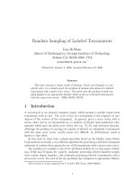
Figure 5 The degree sequence and the nonzero Laplacian eigenvalues of a threshold graph G are
conjugate partitions of 2|E(G)|. In this example, the degrees of the vertices are (5, 3, 2, 2, 1, 1)
and the nonzero eigenvalues of L(G) are (6, 4, 2, 1, 1).
For example, see the graph in Figure 5. The degrees of the vertices are (5, 3, 2, 2, 1, 1) which

is conjugate to the nonzero eigenvalues of the graph’s Laplacian: (6, 4, 2, 1, 1).
Corollary 5.9. Let G be a threshold graph that is not a complete graph. Then its algebraic
connectivity equals its minimum degree, i.e., λ
2
(G) = δ(G).
Note that λ
2
(K
n
) = n but δ(K
n
) = n − 1.
Proof. Let G  K
n
be a threshold graph on n vertices and let 0 = λ
1
 λ
2
 ···  λ
n
be the
eigenvalues of its Laplacian.
If G is not connected, then δ(G) = λ
2
(G) = 0.
Otherwise, G is connected and let s = seq(G). Because G is not complete, s contains at
least one zero. The vertex of smallest degree corresponds to the last zero in s. Its degree is the
number of 1s to its right, which is the number of vertices of maximum degree. Since there are
δ vertices of maximum degree, the last column in the Ferrer’s conjugate has δ boxes, and so
λ

2
= δ. 
Corollary 5.10. Let G be an instance of a random threshold graph on n vertices. Then
Pr{λ
2
(G) = i} =













1/2
n−1
for i = n,
1/2
i+1
for 0  i  n − 2, and
0 otherwise.
In particular E[λ
2
] = 1.
Proof. Immediate from Corollaries 5.6 and 5.9 and the fact that λ

2
(K
n
) = n. 
We can also deduce from Theorem 5.8 that the largest eigenvalue of a threshold graph G
equals |V(G)| − i(G) where i(G) is the number of isolated vertices in G whose distribution is
given in Proposition 5.26.
the electronic journal of combinatorics 16 (2009), #R130 17
Another degree property that can be readily deduced from the creation sequence is the num-
ber of distinct degrees in a threshold graph.
Proposition 5.11. Let G be a threshold graph and let s = seq(G) be its creation sequence. The
number of contiguous blocks of 1s and 0s equals the number of different degrees in G.
Proof. If seq(G) is entirely 0s or 1s, then the graph is either edgeless or complete, respectively.
In either case, all vertices have the same degree.
Otherwise s consists of alternating blocks of 0s and 1s. Note that all vertices within a
contiguous run have the same degree. Furthermore, the one vertex that does not correspond to
an entry in s has the same degree as the vertices in the first block. 
Proposition 5.12. Let G be an instance of a random threshold graph on n vertices and let g
denote the number of distinct degrees in G. Then, for 1  i  n − 1 we have
Pr{g = i} =
1
2
n−2

n − 2
i − 1

.
Proof. We count the number of creation sequences the i runs. The first bit can be either zero
or one (2 choices). After that, we select i − 1 locations from the n − 2 “spaces” between the

bits to show where a block of 1s changes to 0s and vice versa. Hence there are 2

n−2
i−1

creation
sequences with i runs, and the result follows. 
It follows that the expected number of distinct degrees in a random threshold graph on n
vertices is
E[g] =
1
2
n−2
n−1

i=1
i

n − 2
i − 1

=
n
2
.
5.2 Chromatic number
Because threshold graphs are perfect (see, for example, [9]) we can deduce information about
the chromatic number from the clique number which is, in turn, directly available from the
creation sequence.
Proposition 5.13. Let G be an instance of a random threshold graph on n  1 vertices. Then,

the chromatic number and the clique number of G have the following distribution with support
[n]:
Pr{χ(G) = k} = Pr{ω(G) = k} =

n − 1
k − 1

/2
n−1
for 1  k  n.
Proof. Threshold graphs are perfect. Therefore, the chromatic number is the size of the maxi-
mum clique of the graph. However, the size of the maximum clique is one more than the number
of 1s in the creation sequence. This implies that for 1  k  n, Pr{χ(G) = k} = Pr{ω(G) = k} =

n−1
k−1

/2
n−1
. 
the electronic journal of combinatorics 16 (2009), #R130 18
Corollary 5.14. Let G be an instance of a random threshold graph on n  1 vertices. Then, the
independence number of G has the following distribution with support [n]:
Pr{α(G) = k} =

n − 1
k − 1

/2
n−1

for 1  k  n.
Proof. This follows from the fact that α(G) = ω(G). 
Proposition 5.15. Let G be an instance of a random threshold graph. Then, the expected
chromatic number of G, and thus the expected clique number of G, is
n+1
2
.
Proof. By Proposition 5.13,
E[χ(G)] =
1
2
n−1
n

k=1
k

n − 1
k − 1

=
n + 1
2
. 
Corollary 5.16. Let G be an instance of a random threshold graph. Then, the expected inde-
pendence number of G is
n+1
2
.
Proof. Apply Proposition 5.15 and the fact that α(G) = ω(G). 

5.3 Cycles
Proposition 5.17. Let G be an instance of a random threshold graph on n vertices. Then,
Pr{G is acyclic} =
n
2
n−1
.
Proof. Let s = seq(G). Because G is a threshold graph, then by Theorem 2.5, it cannot contain
C
4
as an induced subgraph. Thus, G contains a cycle if and only if it contains K
3
as an induced
subgraph. However, this occurs if and only if there are at least two 1s in s.
Thus,
Pr{G is acyclic} = Pr{s has at most one 1} =

n−1
0

+

n−1
1

2
n−1
=
n
2

n−1
. 
Corollary 5.18. Let G be an instance of a random threshold graph on n vertices. Then, the
probability G has a cycle is 1 −n/2
n−1
. 
Notice that, as n goes to infinity, the probability that G has a cycle goes to 1.
Next, we consider the probability that a random threshold graph is Hamiltonian. There is
a nice connection between Hamiltonicity and a threshold graph’s creation sequence. For more
background on Hamiltonian threshold graphs, see [12].
For a sequence s of 1s and 0s, let u
k
(s) be the number of 1s in the last k bits and z
k
(s) be the
number of 0s in the last k bits.
Definition 5.19. Let G be a graph and c(G) denote the number of connected components of G.
We say that G is tough if for every nonempty subset S ⊆ V(G) we have c(G − S )  |S |.
the electronic journal of combinatorics 16 (2009), #R130 19
Figure 6 The (b)⇒(c) case for Theorem 5.20: toughness implies the strict partial Dyck property.
At some point k, we have u
k
(s)  z
k
(s) (illustrated by the dotted box). If S is the set of vertices
corresponding to the 1s in the box, then c(G −S) > |S |.
Note that a tough graph with three or more vertices must be connected.
Theorem 5.20. Let G be a threshold graph with n  3 vertices. The following are equivalent:
(a) G is Hamiltonian.
(b) G is tough.

(c) If s = seq(G), then u
k
(s) > z
k
(s) for all 1  k  n −1.
The condition u
k
(s) > z
k
(s) for all k means that the reversal of s (i.e., s
n−1
s
n−2
. . . s
1
) satisfies
the strict partial Dyck property; see Appendix A.
Proof. (a) ⇒ (b): This is well-known.
(b) ⇒ (c): Suppose G is tough. Label the vertices of G by the integers 0 through n − 1 so that
vertex i (with i > 0) corresponds to the i
th
bit of s = seq(G).
Suppose, for contradiction, there is an index k so that u
k
(s)  z
k
(s). Let S be the set of those
vertices corresponding to 1s in the last k bits of s. Note that if we delete S from G, the resulting
graph has at least z
k

(s) + 1 components: the component of G − S containing vertex 0 and the
z
k
(s) isolated vertices. This is illustrated in Figure 6. It follows that
c(G − S)  z
k
(s) + 1 > z
k
(s)  |S |
contradicting the fact that G is tough.
(c) ⇒ (a): Suppose that s = seq(G) satisfies u
k
(s) > z
k
(s) for all k with 1  k  n − 1. This
implies that the last two bits of s are both 1s.
We prove that G is Hamiltonian by induction on the number of vertices, n.
In case n = 3, then seq(G) = 11 and so G = K
3
which is Hamiltonian. In case n = 4, then
seq(G) = 111 or 011. In the first case G = K
4
and in the second case G = K
4
−e, both of which
are Hamiltonian.
the electronic journal of combinatorics 16 (2009), #R130 20
Figure 7 Induction step in (c)⇒(a).
n − 1
n − 2

j
C
x
We now assume the theorem has been shown for all graphs with fewer than n vertices (where
we may assume n  5), and let G be a threshold graph with n vertices that satisfies condition
(c).
Without loss of generality, we assume the vertices of G are numbered from 0 to n − 1
corresponding to their position in the creation sequence s = seq(G). If s does not contain any
zeros, then G = K
n
which is Hamiltonian. Otherwise, let j be the index of the last 0 in s; note
that j < n − 2.
Let H be the graph formed by deleting vertices j and n − 1 from G. Observe that H is a
threshold graph whose creation sequence is formed from s by deleting bits j and n − 1. One
checks that H’s creation sequence satisfies property (c) and so, by induction, H is Hamiltonian.
Fix a Hamiltonian cycle C of H and let x be a vertex of H that is adjacent to vertex n −2 on
the cycle C. (See Figure 7.) Note that because the last two bits of s are 1s, vertices n − 2 and
n − 1 are adjacent to both j and x. Thus, if we delete the edge {x, n − 2} from C and insert the
path x ∼ n −1 ∼ j ∼ n −2 in its stead, we create a Hamiltonian cycle in G. 
Theorem 5.21. Let G be an instance of a random threshold graph with n  3 vertices. Then
Pr{G is Hamiltonian} =
1
2
n−1

n − 2
⌊(n − 2)/2⌋

∼
1

√
2πn
.
Proof. The number of sequences of length n − 1 that satisfy condition (c) of Theorem 5.20
is

n−2
⌊(n−2)/2⌋

. This is shown in Proposition A.2. The asymptotic value follows from a routine
application of Stirling’s formula. 
5.4 Perfect matchings
The existence of a perfect matching in a threshold graph is equivalent to a condition that is
similar to that for a Hamiltonian cycle. Recall that for a sequence s of 1s and 0s that u
k
(s) and
z
k
(s) denote the number of 1s and 0s, respectively, in the last k bits of s. We have the following
result that is analogous to Theorem 5.20.
Theorem 5.22. Let G be a threshold graph on n vertices with n even and let s = seq(G). Then
G has a perfect matching if and only if u
k
(s)  z
k
(s) for all k.
the electronic journal of combinatorics 16 (2009), #R130 21
Proof. First, suppose that for some k, u
k
(s) < z

k
(s). Let S be the set of vertices corresponding
to the 1s in the last k bits of s, so |S | = u
k
(s). Note that G − S contains z
k
(s) isolated vertices
plus (perhaps) other odd components. Therefore, by Tutte’s theorem G does not have a perfect
matching.
Conversely, suppose that for all k, u
k
(s)  z
k
(s). We assume that the vertices V(G) are
numbered from 0 to n −1 with vertex i > 0 corresponding to the i
th
bit in s. Let
U = {v : s
v
= 1} ∪ {0} and Z = { v : s
v
= 0}.
Note that U is a clique and Z is an independent set.
Claim. G contains a matching M of edges between U and Z that saturates Z.
Proof of claim. Consider the bipartite graph G
′
consisting of all vertices of G and
all edges of G with one end in Z and the other in U. Let Y ⊆ Z. The set of neighbors
of Y, N(Y) = {u ∈ U : u ∼ y ∃y ∈ Y}, corresponds exactly to the set of all 1s in s to
the right of position y for y ∈ Y. Since u

k
(s)  z
k
(s) for all k, we have |N(Y)|  |Y|
for all Y ⊆ Z. Therefore, by Hall’s theorem, G
′
has a matching M that saturates
Z. 
Finally, we can extend M to a perfect matching since all vertices unsaturated by M (which
are necessarily even in number) lie in the clique U. 
Theorem 5.23. Let n be an even integer and let G be an instance of a random threshold graph
on n vertices. Then
Pr{G has a perfect matching} =
1
2
n−1

n − 1
⌊(n − 1)/2⌋

∼

2
πn
.
Proof. From Theorem 5.22, G has a perfect matching if and only if s = seq(G) is the reverse of
a partial Dyck sequence of length n−1 (see Appendix A). By Proposition A.1 there are

n−1
⌊(n−1)/2⌋


such sequences. The asymptotic expression follows from Stirling’s formula. 
5.5 Edges and extremal vertices
Proposition 5.24. Let G be an instance of a random threshold graph on n vertices, m denote
the number of edges of G, and Q(k, ℓ) denote the number of partitions of k into distinct parts
whose largest part is less than or equal to ℓ. Then, for 0  i 

n
2

, we have that Pr{m = i} =
Q(i, n − 1)/2
n−1
.
Proof. Let s = seq(G). Then,
m =
n−1

j=1
s
j
· j. (2)
Thus, a creation sequence results in a graph with i edges whenever i can be written as the sum
of distinct integers between 1 and n − 1. There are Q(i, n − 1) ways to do this and 2
n−1
creation
sequences total. The result follows. 
the electronic journal of combinatorics 16 (2009), #R130 22
Proposition 5.25. Let G be an instance of a random threshold graph. Then, the expected
number of edges of G is E[m] =

1
2

n
2

. Also, the variance of the number of edges is Var(m) =
n(n−1)(2n−1)
24
.
Proof. Let s = seq(G). Since for all i we have E[s
i
] =
1
2
, equation (2) gives
µ = E[m] = E







n−1

i=1
s
i
· i








=
n−1

i=1
i
2
=
1
2

n
2

.
Using the independence of the s
i
and taking the variance of equation (2), we obtain
σ
2
= Var[m] = Var








n−1

i=1
s
i
· i







=
n−1

i=1
Var[s
i
] · i
2
=
n−1

i=1
i

2
4
=
n(n − 1)(2n − 1)
24
. 
It is interesting to note that an Erd˝os-R´enyi random graph with p =
1
2
has the same expected
number of edges, but the variance of the number of edges is on the order of n
2
while the variance
for a random threshold graph is on the order of n
3
.
Later (§5.6) we show that (m − µ)/σ converges to a normal distribution.
Next, we consider the number of isolated and universal vertices of a random threshold graph.
For a graph G, we let i(G) denote the number of isolated vertices of G and let u(G) denote the
number of universal vertices of G.
Proposition 5.26. Let G be an instance of a random threshold graph on n vertices. Then, the
number of isolated vertices of G has the following distribution:
Pr{i(G) = j} =














1/2
n−1
for j = n,
1/2
j+1
for 0  j  n −2, and
0 otherwise.
Proof. First, notice that it is impossible to have n−1 isolated vertices. So, Pr{i(G) = n−1} = 0.
Now, let s = seq(G). Then, i(G) = n if and only if s
i
= 0 for all i. Therefore, Pr{i(G) = n} =
1
2
n−1
.
For 0  j  n − 2, we notice that i(G) = j if and only if s
n−1−j
= 1 and the last j bits equal 0.
Thus, we have Pr{i(G) = j} =
1
2
j+1
. 
Corollary 5.27. Let G be an instance of a random threshold graph on n vertices. Then the

number of universal vertices of G has the following distribution:
Pr{u(G) = j} =













1/2
n−1
for j = n,
1/2
j+1
for 0  j  n − 2, and
0 otherwise.
Proof. Notice that i(G) = u(G). The result follows from Proposition 5.26. 
the electronic journal of combinatorics 16 (2009), #R130 23
Proposition 5.28. Let G be an instance of a random threshold graph. Then E[i(G)] = E[u(G)] =
1.
Proof. Note that i(G) and u(G) have the same distribution, so it is enough to find the expected
value of just one of them.
E[i(G)] =
n

2
n−1
+
n−2

j=1
j ·
1
2
j+1
=
n
2
n−1
+

1 −
n
2
n−1

= 1. 
We note that the existence of a common neighbor between two vertices increases the like-
lihood that those vertices are adjacent. This clustering phenomena may be a reason that some
have considered random threshold graphs as a model for social networks [11]. Here is a formal
statement.
Proposition 5.29. Let a, b, c be distinct vertices of a random threshold graph. Then
Pr{a ∼ b | a ∼ c ∼ b} > Pr{a ∼ b}.
Proof. Using Example 3.2, we have
Pr{a ∼ c ∼ b} = Pr{a ∼ c ∼ b and a ∼ b} + Pr{a ∼ c ∼ b and a  b} =

1
4
+
1
12
=
1
3
.
Therefore,
Pr{a ∼ b | a ∼ c ∼ b} =
Pr{a ∼ b and a ∼ c ∼ b}
Pr{a ∼ c ∼ b}
=
1/4
1/3
=
3
4
>
1
2
= Pr{a ∼ b}. 
5.6 Small induced subgraphs
Let H be a threshold graph. We are interested in determining the number of copies of H ap-
pearing in a random threshold graph G. Specifically, we wish to understand the behavior of the
random variable N
H
(G) which we define to be the number of induced copies of H. This is an
extension of Proposition 5.25 in which H = K

2
. Of course, if H is not a threshold graph, then
N
H
= 0.
With a modest abuse of notation, we also write N
H
(x) to mean N
H
[Γ(x)], i.e., the number of
copies of H in the threshold graph represented by x.
Theorem 5.30. Let H be a threshold graph on h vertices and let N
H
be the number of induced
copies of H in an n-vertex random threshold graph. Then the expected value of N
H
is E [N
H
] =

n
h

/2
h−1
and its variance is Var(N
H
) ∼ cn
2h−1
for some constant c > 0.

For example, for H = K
2
, Proposition 5.25 gives
E(N
H
) =
1
2

n
2

and Var(N
H
) =
n(n − 1)(2n − 1)
24
∼
1
12
n
3
.
the electronic journal of combinatorics 16 (2009), #R130 24
Proof. Let A be an h-element subset of [n] and define X
A
to be the indicator random variable
that G[A] (the induced subgraph of the random threshold graph G on vertex set A) is isomorphic
to H, i.e., X
A

= 1{G[A]  H}. Hence N
H
=

X
A
.
As there are h!/|Aut(H)| different ways in which H might be realized on a set of h vertices,
we have
E[X
A
] = Pr{G[A]  H} =
h!
|Aut(H)|
Pr{H} =
h!
|Aut(H)|
·
|Aut(H)|
2
h−1
h!
=
1
2
h−1
.
It follows that E[N
H
] =


n
h

/2
h−1
by linearity of expectation.
It is useful to present a second derivation for E[N
H
] based on creation sequences. In this
approach, we prepend a “wild card” symbol (∗) to all creation sequences to stand for the first
vertex in the graph. This wild card can be considered either a 1 or a 0; it does not matter as it is
the first vertex in the creation list.
Let s
H
be the creation sequence for the graph H (including the initial wild card) and let S
be a random creation sequence (an initial ∗ followed by a random sequence of n −1 1s and 0s).
Then the number of induced copies of H in the random threshold graph generated by S equals
the number of h-long subsequences of S that match s
H
where the ∗ in s
H
can match any symbol
in S.
Therefore, given a fixed subset A of h entries in S , the probability that those entries match s
H
is 1/2
h−1
, and so Pr{X
A

= 1} = 1/2
h−1
. As there are

n
h

such subsets we have E[N
H
] =

n
h

/2
h−1
.
For the second claim, note that
Var(N
H
) = Var








A

X
A







=

A

B
Cov(X
A
, X
B
) =
h

i=0

A,B:
|A∩B|=i
Cov(X
A
, X
B
) (3)

where the double sums are over all A, B ⊂ [n] with |A| = |B| = h, but the second is organized by
the size of the intersection of A and B. Note that the number of summands in which |A ∩ B| = i
is

n
h

h
i

n − h
h − i

= Θ(n
2h−i
).
Note that when A and B are disjoint, then Cov(X
A
, X
B
) = 0. When i > 1, this expression is
o(n
2h−1
). We therefore concentrate solely on the terms Cov(X
A
, X
B
) in (3) for which |A ∩B| = 1.
There are


n
2h−1

ways to choose the elements of A ∪ B for which |A ∩ B| = 1. For each such
union, there are

2h−1
h

h choices for the ordered pair (A, B) and the restricted sum of Cov(X
A
, X
B
)
is the same for all possible choices of A ∪ B of size 2h − 1. That is, we have

|A∩B|=1
Cov(X
A
, X
B
) =

n
2h − 1


A∪B=[2h−1]
|A∩B|=1
Cov(X

A
, X
B
) (4)
We consider a particular term in the second sum in (4). Let A = {a
1
< a
2
< ··· < a
h
} and
B = {b
1
< b
2
< ··· < b
h
} where A ∪ B = [2h − 1]. Let α, β be the indices of A, B [respectively]
of their unique common element; that is, a
α
= b
β
.
the electronic journal of combinatorics 16 (2009), #R130 25