Báo cáo toán học: "Some gregarious cycle decompositions of complete equipartite graphs" ppsx

Some gregarious cycle decompositions of
complete equipartite graphs
Benjamin R. Smith
Department of Mathematics
University of Queensland
Qld 4072, Austr alia

Submitted: Aug 17, 2009; Accepted: Nov 3, 2009; Pu blished: Nov 13, 2009
Mathematics S ubject Classification: 05C38, 05C51
Abstract
A k-cycle decomposition of a multipartite graph G is said to be gregarious if each
k-cycle in the decomposition intersects k distinct partite sets of G. In this paper we
prove necessary and sufficient conditions for the existence of such a decomposition
in the case where G is the complete equipartite graph, having n parts of size m,
and either n ≡ 0, 1 (mod k), or k is odd and m ≡ 0 (mod k). As a consequence,
we prove necessary and sufficient conditions for decomposing complete equipartite
graphs into gregarious cycles of prime length.
1 Introduction and p r eliminaries
We begin with some relevant definitions a nd terminology.
Let K
n
denote the complete graph on n vertices a nd K
n
denote the empty graph on n
vertices. For any graph G and any positive integer λ, we denote the multigraph obtained
from G by replacing each of its edges with λ para llel edges by λG.
We denote the k- cycle containing edges v
1
v
2
, v

2
v
3
, . . . , v
k−1
v
k
and v
1
v
k
by
(v
1
, v
2
, . . . , v
k
), or (v
k
, v
k−1
, . . . , v
1
), or by any cyclic shift of these. We denote the k-path
containing edges v
1
v
2
, v

2
v
3
, . . . , v
k
v
k+1
by [v
1
, v
2
, . . . , v
k+1
] or [v
k+1
, v
k
, . . . , v
1
] (hence, in
our terminology, a k-path contains k edges and k + 1 vertices). Similarly, we denote the
directed k-cycle containing directed edges (v
1
, v
2
), (v
2
, v
3
), . . . , (v

k−1
, v
k
) and (v
k
, v
1
) by
(v
1
, v
2
, . . . , v
k
)
D
, or by any cyclic shift of this.
The lexicographic product G ∗ H of graphs G and H is the graph with vertex set
V (G) × V (H), and with an edge joining (g
1
, h
1
) to (g
2
, h
2
) if and only if g
1
g
2

∈ E(G),
or g
1
= g
2
and h
1
h
2
∈ E(H). For our purposes we will primarily be concerned with
the electronic journal of combinatorics 16 (2009), #R135 1
lexicographic products of the form G ∗ K
m
, for some G and m. We note that for all
graphs G and positive integers a and ℓ,
G ∗ K
aℓ
∼
=
(G ∗ K
a
) ∗ K
ℓ
∼
=
(G ∗ K
ℓ
) ∗ K
a
.

A subgraph of a multipartite graph G is said to be gregarious in G (or simply gregarious
when G is clear) if each of its vertices lies in a different partite set of G. In order to apply
this definition, it must be clear what the partite sets of G are. With this in mind we
adopt the following convention.
Suppose G is a graph on n vertices, and a a nd ℓ are positive integers. Through-
out this paper, unless otherwise specified, we assume the graph G ∗ K
aℓ
has vertex set
{v
1
, v
2
, . . . , v
aℓ
| v ∈ V (G)}, and an edge joining u
i
and v
j
in G ∗ K
aℓ
if and only if there is
an edge joining u and v in G. The partite sets of G ∗ K
aℓ
are the n sets {v
1
, v
2
, . . . , v
aℓ
},

v ∈ V (G). However, we may occasionally choose to express the lexicographic product of
G and K
aℓ
as G ∗ K
a(ℓ)
, or indeed G ∗ K
ℓ(a)
. In the first case, it is assumed that there
is a further partitioning of each o f the sets {v
1
, v
2
, . . . , v
aℓ
} into a subsets, each of size ℓ.
It is these na sets of size ℓ which are considered the partite sets of G ∗ K
a(ℓ)
. Similarly
in the second case, it is assumed that there is a further partitioning of each of the sets
{v
1
, v
2
, . . . , v
aℓ
} into ℓ subsets, each of size a. It is these nℓ sets of size a which are con-
sidered the partite sets of G ∗ K
ℓ(a)
. Note that this means a given subgraph H may be
gregarious in G ∗ K

a(ℓ)
, but not gregarious in G ∗ K
aℓ
.
A decomposition of a graph G is a collection of subgraphs of G whose edge-sets partition
the edge-set of G. Let H = {H
∞
, H
∈
, . . . , H
⊔
} be a family of mutually nonisomorphic
nontrivial graphs. An H-decomposition of G is a decomposition, D say, of G such that
• for each D ∈ D there is some H
i
∈ H with D
∼
=
H
i
; and
• for each H
i
∈ H there is some D ∈ D with H
i
∼
=
D.
If H = {H} we often refer to such a decomposition as simply an H-decomposition. A
decomposition of a multipartite graph G is said to be gregarious if each of the subgraphs

in the decomposition is gregar io us in G.
In this paper we will be concerned with gregarious k-cycle decompositions of K
n
∗K
m
,
the complete equipartite graph having n parts of size m. Note that every vertex in K
n
∗K
m
has degree (n − 1)m and the total number of edges in K
n
∗ K
m
is n(n − 1)m
2
/2. Hence,
obvious necessary conditions for the existence of such a decomposition are that
• n  k  3 ;
• (n − 1)m is even; and
• n(n − 1)m
2
≡ 0 (mod 2k).
The study of gregarious cycle decompositions is relatively new and thus, compared to
“nongregarious” cycle decompositions, few results are known. Of course 3-cycle decom-
positions of complete equipartite graphs are necessarily gregarious and so by Hanani [5],
the electronic journal of combinatorics 16 (2009), #R135 2
the above necessary conditions are sufficient when k = 3. Sufficiency of these conditions
has also been proved by Billington and Hoffman [2] when k = 4, by Smith [9] when k = 5
and by Billington, Hoffman and Smith [4] when k ∈ {6 , 8}. More generally, in [3] Billing-

ton, Hoffman and Rodger prove there exists a resolvable gregarious n-cycle decomposition
of K
n
∗ K
m
if and only if (n, m) = (3, 2) or (3, 6); that is, the cycles in the decomposition
can be partitioned into sets in such a way that the cycles in each set induce a 2-factor
of K
n
∗ K
m
. (Note that there exists nonresolvable gregarious 3-cycle decompositions of
both K
3
∗ K
2
and K
3
∗ K
6
.) In this paper, using the various new construction techniques
presented in Section 2, we prove sufficiency of the above necessary conditions in cases
where either n ≡ 0, 1 (mod k), or k is odd and m ≡ 0 (mod k). More formally, the main
result (split into two parts) of this paper is the following.
Theorem 1.1 Suppose n, m and k are positive integers with k  3. Necess ary conditions
for the exi s tence of a gregarious k-cycle decompos i tion of K
n
∗K
m
are that n  k, (n−1)m

is even and n(n − 1)m
2
≡ 0 (mod 2k).
(i) These conditions are sufficient whe never n ≡ 0, 1 (mod k).
(ii) These conditions are sufficient whenever k is odd and m ≡ 0 (mod k).
Part (i) of the above theorem is proved in Section 3, while part (ii) is proved in Section
4. Also, Theorem 1 .1 has the following nice corollary.
Corollary 1.2 Suppose n, m and p are positive integers with p an odd prime. Then there
exists a gregarious p-cycle decomposition of K
n
∗ K
m
if and only if n  p, (n − 1)m is
even and n(n − 1)m
2
≡ 0 (mod 2p).
Proof Since n(n − 1)m
2
≡ 0 (mod 2p) and p is prime, we must have either n ≡ 0, 1
(mod p) or m ≡ 0 (mo d p). The result then follows by Theorem 1.1. 
Hence, for arbitrary n and m, Corollary 1.2 gives the first known infinite family of
values of k for which the obvious necessary conditions for the existence of a gregarious
k-cycle decomposition of K
n
∗ K
m
are also sufficient.
2 Some new decomposition techniques
In this section we introduce some new techniques for obtaining gregarious cycle decompo-
sitions of complete equipartite graphs from cycle decompo sitions of related multigraphs.

The techniques used are similar to those introduced in [11].
We begin with the following definition.
Definition 2.1 Suppose D = {H
1
, H
2
, . . . , H
t
} is a decomposition of λG. A λ-weight
function on D is any function ω which assigns an integer label, from the set {0, 1, . . . , λ−1},
to each edge of the g r aphs H
1
, H
2
, . . . , H
t
, in such a way that distinct copies of the same
edge receive distinct lab els. (Hence for each ℓ ∈ {0, 1, . . . , λ − 1}, the edges labelled ℓ
induce a copy of the graph G.) 
the electronic journal of combinatorics 16 (2009), #R135 3
Note that the above definition is a specialisation of a more general type of “weight
function” first described in [11].
The next lemma shows how a cycle decomposition of the gra ph 2G, t ogether with a
2-weight function, can be used to generate a gregarious cycle decomposition of the graph
G ∗ K
2
when certain extra conditions on the original decomposition are satisfied.
Lemma 2.2 Suppose there exists a k-cycle decomposition of 2G which can be partitioned
into pairs of cycles in such a way that the cycles in each pair share two adjacent edges .
Then there exists a gregarious k-cycle decomposition of G ∗ K

2
.
Proof Let D be a k-cycle decomposition of 2G which satisfies the conditions of the
lemma and let ω be any 2-weight function on D. Recall that G ∗ K
2
is the graph obta ined
from G by replacing each vertex v in G with the set of vertices {v
1
, v
2
}, and each edge uv
in G with the edges u
1
v
1
, u
1
v
2
, u
2
v
1
and u
2
v
2
.
For each k-cycle C ∈ D we generate a subgraph, denoted by
ˆ

C, of G∗K
2
by associating
each vertex v in C with the set of vertices {v
1
, v
2
}, and each edge uv in C having label
ℓ (under the f unction ω) with the pair of edges u
1
v
1+ℓ
and u
2
v
2+ℓ
(subscripts calculated
mod 2). Note that
ˆ
C is either a single 2k- cycle (if C contains an odd number of edges
labelled 1), or two vertex disjoint k-cycles which are gregarious in G∗K
2
(if C contains an
even number of edges labelled 1). Since ω is a 2-weight function, the graphs
ˆ
C together
decompose G ∗ K
2
. Hence we need only show that, if C and C
′

are any “pair” of cycles
from the partition of D, then the graph
ˆ
C ∪
ˆ
C
′
admits a decomposition into k-cycles which
are gregarious in G ∗ K
2
.
Let uv and vw be the two adjacent edges shared by C and C
′
. Then
ˆ
C ∪
ˆ
C
′
contains
the edges u
i
v
j
and v
i
w
j
for each i, j ∈ {1, 2}. Let H be the subgraph of
ˆ

C ∪
ˆ
C
′
spanned
by these edges, and let H
′
be the complement of H in
ˆ
C ∪
ˆ
C
′
. (Hence {H, H
′
} is a
decomposition of
ˆ
C ∪
ˆ
C
′
.) Then for some a, b ∈ {1, 2 } the graph H
′
decomposes into four
gregarious (k − 2)-paths:
L
1
=[w
a

, . . . , u
1
]; L
2
=[w
a+1
, . . . , u
2
]; L
3
=[w
b
, . . . , u
1
]; L
4
=[w
b+1
, . . . , u
2
].
Now H decomposes into the four gregarious 2-paths:
P
1
=[u
1
, v
1
, w
a

]; P
2
=[u
2
, v
1
, w
a+1
]; P
3
=[u
1
, v
2
, w
b
]; P
4
=[u
2
, v
2
, w
b+1
].
The result then follows by adjoining the (k − 2)-path L
i
to the 2-path P
i
, for each i ∈

{1, 2, 3, 4}. 
Note t hat the “pairing” condition in Lemma 2.2 means there must be an even number
of cycles in the decomposition of 2 G . In fact, it is easy to see that we can relax this
condition slightly and obtain the following generalisation.
Lemma 2.3 Suppose there exists a k-cycle decomposition of 2G which can be partitioned
into two parts, say D
1
and D
2
, so that every cycle in D
1
shares an edge with some cycle
in D
2
, and D
2
can be partitioned into pairs of cycles in such a way that the cycles in each
pair share two adjacent edges. Then there exists a gregarious k-cycle decom position of
G ∗ K
2
.
the electronic journal of combinatorics 16 (2009), #R135 4
Proof Let D = D
1
∪ D
2
. We show there exists a 2-weight function ω on D with the
property that each cycle in D
1
contains an even number of edges labelled 1 (under ω).

Using the notation defined in the proof of Lemma 2.2, the result then follows since for
each C ∈ D
1
, the graph
ˆ
C consists of two k-cycles which are gregarious in G ∗ K
2
, and
for each “pair” of cycles C and C
′
in the partition of D
2
the graph
ˆ
C ∪
ˆ
C
′
admits a
decomposition into k-cycles which are g rega r io us in G ∗ K
2
(using the method described
in the proof of Lemma 2.2).
Let ω be any 2-weight function on D. If each cycle in D
1
contains an even number
of edges labelled 1 we are done. If not, we modify ω as follows. Suppose C ∈ D
1
and
C contains an odd number of edges labelled 1. Now C contains an edge, e say, which is

also contained in some cycle, C
′
say, in D
2
. We switch the label on the edge e in C from
either 0 to 1, or vice-versa. We then do the same for the copy of the edge e in C
′
. Hence
the resulting edge labelling still induces a 2-weight function on D. Moreover, the cycle
C now contains an even number o f edges labelled 1 and we have not affected the edge
labellings of any other cycles in D
1
. We repeat this process for each cycle in D
1
having
an odd number of edges labelled 1. The r esulting edge labelling then induces a 2-weight
function on D with the required property. 
In order to more fully exploit these newly defined λ-weight functions we also introduce
the idea of the “sum-weight” of a cycle. (Again, this concept was originally defined in
[11].)
Definition 2.4 Suppose C is a cycle in the graph G. Suppose furthermore that

G is the
graph obtained by orienting the edges of G in some way, and that ω is a function which
assigns an integer label ω(e) to each edge e in the cycle C. We let

C be a directed cycle
formed by orienting the edges of C, and for each edge e in C we denote the corresponding
directed edge in


C by e
′
. (Note that there are two possible choices for

C, and that

C
need not be a subgraph of

G.) The sum-weight with respect to

G under the function ω o f
the cycle C, is then defined to be the absolute value of the sum, over all edges e in C, of
f(e
′
)ω(e), where
f(e
′
) =

1, if e
′
is an edge in

G;
−1, otherwise.
Note that taking the “absolute value” ensures that the sum-weight is independent of the
choice of

C. Furthermore, when bo t h


G and ω are clear, we will often refer simply t o
the sum-weight of the cycle C, rather than the sum-weight with respect to

G under the
function ω. 
In [11] we defined the notion of an unbalanced λ-weight function on a cycle decom-
position of a graph λG. These functions have the property that under some particular
orientation of the edges of G, say

G, each cycle in the decomposition of λG has sum-weight
coprime to λ. Hence each k-cycle C in t he decomposition of λG can be used to generate
a λk-cycle in the graph G ∗ K
λ
by associating each vertex v in C with the partite set
A
v
= {v
1
, v
2
, . . . , v
λ
}, and each edge uv labelled ℓ in C with the matching between A
u
the electronic journal of combinatorics 16 (2009), #R135 5
and A
v
consisting of the edges u
1

v
1+ℓ
, u
2
v
2+ℓ
, . . . , u
λ
v
λ+ℓ
if (u, v) is an edge in

G, or the
edges v
1
u
1+ℓ
, v
2
u
2+ℓ
, . . . , v
λ
u
λ+ℓ
if (v, u) is an edge in

G. The fact that the sum-weight of
C is coprime to λ ensures that the k matchings f orm a single λk-cycle in G ∗ K
λ

, rather
than a collection of disjoint cycles whose lengths sum to λk. Since here we are interested
in gregarious cycle decompositions, we will instead be concerned with λ-weight functions
under which each cycle in a decomposition of λG has sum-weight a multiple of λ. In
this case, a k-cycle in the decomposition of λG will generate, using the same method as
described above, a subgraph in G ∗ K
λ
consisting of λ pairwise vertex-disjoint gregarious
k-cycles. We call such a function a balanced λ-weight function. More formally we define
this as fo llows.
Definition 2.5 Suppose D is a cycle decomposition of λG a nd ω is a λ- weight function
on D. Then ω is said to be balanced if, under some orientation of the edges of G, each
cycle in D has sum-weight a multiple of λ. 
The following lemma proves that such functions do indeed generate gregarious cycle
decompositions.
Lemma 2.6 Suppose D is a k-cycle decomposition of λG and ω is a balanced λ- weight
function on D. Then there exists a gregarious k-cycle decomposition of G ∗ K
λ
.
Proof Let

G be the particular orientation of the edges of G under which ω is balanced.
For each k-cycle C ∈ D we generate a subgraph in G ∗ K
λ
by associating each vertex v in
C with the part ite set A
v
= {v
1
, v

2
, . . . , v
λ
}, and each edge uv in C having label ℓ (under
the function ω) with the matching between partite sets A
u
and A
v
consisting of the edges
u
1
v
1+ℓ
, u
2
v
2+ℓ
, . . . , u
λ
v
λ+ℓ
if (u, v) is an edge in

G, or the edges v
1
u
1+ℓ
, v
2
u

2+ℓ
, . . . , v
λ
u
λ+ℓ
if (v, u) is an edge in

G. Hence each of these subgraphs is a 2-regular graph on λk vertices.
In fact, since the sum-weight of each cycle in D is a multiple of λ, each of these subgraphs
necessarily consists of λ pairwise vertex-disjoint k-cycles, each of which is gregarious in
G ∗ K
λ
. Furthermore, since ω is a λ-weight function, the collection of all such k-cycles
forms a decomposition of G ∗ K
λ
as required. 
3 The case n ≡ 0, 1 (mod k)
The aim of this section is to prove Theorem 1.1 (i). We make extensive use of the following
three obvious, but surprisingly useful, results.
Lemma 3.1 Suppose there exists a gregarious {H
1
, H
2
, . . . , H
t
}-decomposition of G ∗ K
a
and, for each i ∈ {1, 2 , . . . , t}, there exists a gregarious H-decomposition of H
i
∗K

ℓ
. Then
there ex i sts a gregario us H-decomposition of G ∗ K
aℓ
.
Lemma 3.2 Suppose there ex i sts a {H
1
, H
2
, . . . , H
t
}-decomposition of G ∗ K
a
and, for
each i ∈ {1, 2, . . . , t}, there exists a gregarious H-decompo sition of H
i
∗ K
ℓ
. Then there
exists a g regarious H-decomposition of G ∗ K
a(ℓ)
.
the electronic journal of combinatorics 16 (2009), #R135 6
Lemma 3.3 Suppose there exists a gregarious {H
1
, H
2
, . . . , H
t
}-decomposition of G ∗ K

a
and, f or each i ∈ {1, 2, . . . , t}, there exists an H-decomposition of H
i
∗ K
ℓ
. Then there
exists a g regarious H-decomposition of G ∗ K
ℓ(a)
.
The following is a direct application of Lemma 3.2.
Lemma 3.4 Suppose there exists a k-cycle decomposition of G ∗ K
a
. Then, for each
positive integer ℓ, there exists a gregario us k-cycle decomposition of G ∗ K
a(ℓ)
.
Proof By Lemma 3.2 we need only prove there exists a gregarious k-cycle decomposition
of C ∗ K
ℓ
, where C is a (generic) k-cycle. Suppose C = (1, 2 , . . . , k). If ℓ is even we take
the ℓ
2
cycles (1
i
, 2
j
, . . . , (k − 1)
i
, k
j

), where i, j ∈ {1, 2, . . . , ℓ}. If ℓ is odd we take the ℓ
2
cycles (1
i
, 2
j
, . . . , (k − 1)
j
, k
i◦j
), where i, j ∈ {1, 2, . . . , ℓ} and i ◦ j is the entry in row i
and column j of any (fixed) latin square of order ℓ on the set {1, 2, . . . , ℓ}. It is an easy
exercise to check that these cycles decompose C ∗ K
ℓ
as required. 
We can apply Lemma 3.1 in a similar way and obtain the following easy result.
Lemma 3.5 Suppose there exists a greg arious k-cycle decomposition of G ∗ K
a
. Then,
for each positive integer ℓ, there exists a g regarious k-cycle decomposition of G ∗ K
aℓ
.
We will also make use of some well-known results involving cycle decompositions of
complete graphs and complete equipartite graphs. The first such result, due to Alspach,
Gavlas [1] and Sˇajna [8], gives necessary and sufficient conditions for the existence of a
k-cycle decomposition of the complete graph K
n
.
Theorem 3.6 ([1],[8]) Suppose n and k are positive integers with n  3 and k  3. Then
there exists a k-cycle decomposition of K

n
if and only if n  k, n is odd and n(n − 1) ≡ 0
(mod 2k).
We note that if there exists a k-cycle decomposition of K
n
then, by Lemma 3.4, for
each positive integer m there exists a gregarious k-cycle decomposition of K
n
∗K
m
. Hence
we have the following obvious corollary to Theorem 3.6.
Corollary 3.7 Suppose n, m and k are positive integers with n  3 and k  3. Th e n
there exists a gregarious k-cycle decomposition of K
n
∗ K
m
whenever n  k, n is odd and
n(n − 1) ≡ 0 (mod 2k).
The next theorem follows from a stronger result of Liu [6],[7] involving resolvable
cycle decompositions of complete equipartite graphs. Note that we have removed the
“resolvability” condition from Liu’s original result since we will not be concerned with
that property here (this also allows us to easily remove the “exceptions” from Liu’s original
result).
Theorem 3.8 ([6],[7]) Suppose n, m and k are positive integers with n  3 and k  3.
Then there exists a k-cycle decomposition of K
n
∗ K
m
whenever (n − 1)m is even and

nm ≡ 0 (mod k).
the electronic journal of combinatorics 16 (2009), #R135 7
Combining this result with Lemma 3.4 we have the following easy corollary.
Corollary 3.9 Suppose n, ℓ, a and k are positive integers with n  3 and k  3. Then
there exists a greg arious k-cycle decomposition of K
n
∗ K
ak(ℓ)
whenever (n − 1)ak is even.
We now state a result of Billington et al. [3] involving gregarious k-cycle decompositions
of K
k
∗K
m
. We note, as mentioned in the introduction, that they actually proved necessary
and sufficient conditions for the existence of a resolvable gregarious k-cycle decomposition
of K
k
∗ K
m
however, as already noted, we will not be concerned with this additional
property here.
Theorem 3.10 ([3]) Suppose k and m are positive integ ers with k  3. Then there exists
a gregarious k-cycle decomposition of K
k
∗ K
m
if and only if either k is odd or m is even.
This result has the following simple corollary in the case that k is even.
Corollary 3.11 Suppose n, m and k are posi tive integers with m and k even, and k  4.

Then there exists a gregarious k-cycle decomposition of K
n
∗K
m
whenever n ≡ 0 (mod k).
Proof If n = k the result follows immediately by Theorem 3.10. Suppose then that
n = qk, with q  2. It is easy to see that there exists a {K
k
, K
q
∗ K
k
}-decomposition of
K
n
∼
=
K
qk
∗ K
1
. Moreover, there exist gregarious k-cycle decompositions of K
k
∗ K
m
, by
Theorem 3.10, and of K
q
∗ K
k(m)

, by Corollary 3.9. Hence the result follows by Lemma
3.2. 
Using the techniques developed in Section 1 (in particular Lemma 2.3), we now present
a series of three lemmas (each followed immediately by a corollary) in which we obta in
some useful gregar io us cycle decompositions of complete equipartite graphs having parts
of even size. The first of these decomp ositions deals with cases in which the cycle length
is also even.
Lemma 3.12 Suppose k and m are positive integers with k  4. Then there exists a
gregarious k-cycle decomposition of K
k+1
∗ K
m
whenever k and m are both even .
Proof If k = 4 the result follows from [2]. Suppose then k  6. No te t hat we need
only consider the case m = 2 and the result then follows by Lemma 3.5. Furthermore, in
the case m = 2 we need only give a k-cycle decomposition of 2K
k+1
which satisfies the
conditions of Lemma 2.3. We do this as follows.
Let the vertex set of 2 K
k+1
be Z
k
∪ {∞}, a nd let ρ = (0 1 2 · · · (k − 1))(∞) be a
permutation of order k on V (2K
k+1
). We define the k-cycles C and D on 2K
k+1
by
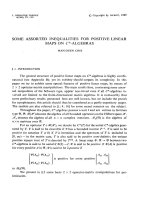
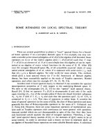
C = (0, 1 , k − 1, 2, k − 2, . . . , k/2 − 1, k/2 + 1, ∞); and

D = (0, 1, 2, . . . , k − 1).
(See for example Figure 1, which shows the cycles C and D in the case k = 16.)
the electronic journal of combinatorics 16 (2009), #R135 8
7
6
5
4
2
1
3
0
∞
8
10
11
12
13
14
15
9 7
6
5
4
2
1
3
0
∞
8
10

11
12
13
14
15
9
Figure 1: The cycles C and D when k = 16
It is a simple exercise to check that D = {D, ρ
0
(C), ρ
1
(C), . . . , ρ
k−1
(C)} is a k-cycle
decomposition of 2K
k+1
. We note that, f or each i ∈ {0, 1, . . . , k/2 − 1}, the cycles ρ
i
(C)
and ρ
i+k/2
(C) both contain the 2-path [i + 1, i − 1, i + 2]. Hence, setting D
1
= {D}
and D
2
= {ρ
0
(C), ρ
1

(C), . . . , ρ
k−1
(C)}, it is easy to see that D satisfies the conditions of
Lemma 2.3 and the result follows. 
Corollary 3.13 Suppose n, m and k are posi tive integers with m and k even, and k  4.
Then there exists a gregarious k-cycle decomposition of K
n
∗ K
m
whenever n  k and
n ≡ 1 (mod k).
Proof If n = k + 1 the result follows immediately by Lemma 3.12. Suppose then that
n = qk +1, with q  2. It is easy to see that there exists a {K
k+1
, K
2
∗K
k
}-decomposition
of K
n
∼
=
K
qk+1
∗K
1
. Moreover, there exist gregarious k-cycle decompositions of K
k+1
∗K

m
,
by Lemma 3.12, and of K
2
∗ K
k(m)
, by Corollary 3.9. Hence the result follows by Lemma
3.2. 
The next result is analo gous to that of Lemma 3.12 in the case that k is odd.
Lemma 3.14 Suppose k and m are positive integers with k  3. Then there exists a
gregarious k-cycle decomposition of K
k+1
∗ K
m
whenever k is odd and m is even .
Proof As in the proof of L emma 3.12, we need only give a k-cycle decomposition of
2K
k+1
which satisfies the conditions of Corollary 2.3. The result then follows for m = 2
by Lemma 2.3, and subsequently for all even m by Lemma 3.5.
Let the vertex set of 2K
k+1
be Z
k
∪ {∞}, and let ρ = (0 1 2 · · · (k − 1))(∞) be
a permutation of or der k on V (2K
k+1
). We then split the problem according to the
congruence of k modulo 4.
the electronic journal of combinatorics 16 (2009), #R135 9

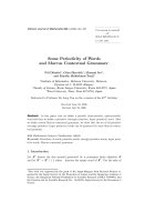
Case I. Suppose k ≡ 1 (mod 4). Let k = 4ℓ + 1 and define the (4ℓ + 1)-cycles C and D
on 2K
4ℓ+2
by
C = (0, 1, 4ℓ, 2, 4ℓ − 1, . . . , ℓ , 3 ℓ + 1 , ℓ + 2, 3ℓ, ℓ + 3, . . . , 2ℓ, 2ℓ + 2, 2ℓ + 1, ∞); and
D = (0, 2 ℓ , 4ℓ, 2ℓ − 1, 4ℓ − 1, . . . , 1, 2ℓ + 1).
(See for example Figure 2, which shows the cycles C and D in the case k = 17.)
1
2
4
0
∞
5
3
7
6
9 8
15
14
13
12
11
10
16 1
2
4
0
5
3
7

6
9 8
15
14
13
12
11
10
16
Figure 2: The cycles C and D when k = 17
It is a simple exercise to check that D = {D, ρ
0
(C), ρ
1
(C), . . . , ρ
4ℓ
(C)} is a k-cycle
decomposition of 2K
4ℓ+2
. We note that, for each i ∈ { 0, 1, . . . , 2ℓ − 1}, the cycles ρ
i
(C)
and ρ
i+2ℓ
(C) both contain the 2-path [∞, i, i + 1]. Hence, setting D
1
= {D, ρ
4ℓ
(C)} and
D

2
= {ρ
0
(C), ρ
1
(C), . . . , ρ
4ℓ−1
(C)}, it is easy to see that D satisfies the conditions of
Lemma 2.3 and the result follows.
Case II. Suppose k ≡ 3 (mod 4). Let k = 4ℓ + 3 and define the (4ℓ + 3)-cycles C and D
on 2K
4ℓ+4
by
C =(0, 1, 4ℓ + 2, 2, 4ℓ + 1, . . . , 3ℓ + 3, ℓ + 1, 3ℓ + 1, ℓ + 2, 3ℓ, . . . , 2ℓ, 2ℓ + 2, 2ℓ + 1, ∞); and
D =(0, 2ℓ + 1, 4ℓ + 2, 2ℓ, 4ℓ + 1, . . . , 1, 2ℓ + 2).
It is a simple exercise to check that D = {D, ρ
0
(C), ρ
1
(C), . . . , ρ
4ℓ+2
(C)} is a k-cycle
decomposition of 2K
4ℓ+4
. We note that, for each i ∈ {0, 1, 2, . . . , 2ℓ − 1} , the cycles ρ
i
(C)
and ρ
i+2ℓ+2
(C) both contain the 2-path [∞, i, i + 1]. Hence, setting D

1
= {D, ρ
2ℓ+1
(C)}
and D
2
= {ρ
0
(C), ρ
1
(C), . . . , ρ
2ℓ
(C), ρ
2ℓ+2
(C), ρ
2ℓ+3
(C), . . . , ρ
4ℓ+2
(C)}, it is easy to see
that D satisfies the conditions of Lemma 2.3 and the result follows. 
Corollary 3.15 Suppose n, m and k are positive integers with n and m even, k odd and
k  3. Then there exists a gregarious k-cycle decompos ition of K
n
∗ K
m
whenever n  k
and n ≡ 1 (mod k).
the electronic journal of combinatorics 16 (2009), #R135 10
Proof If k = n − 1, the result follows immediately from Lemma 3.14. Suppose then
n = qk + 1, with q  3 and q odd (since n is even). It is easy to see that there exists

a {K
k+1
, K
q
∗ K
k
}-decomposition o f K
n
∼
=
K
qk+1
∗ K
1
. Moreover, there exist gregarious
k-cycle decompositions of K
k+1
∗ K
m
, by Lemma 3.14, and of K
q
∗ K
k(m)
, by Corollary
3.9. Hence the r esult follows by Lemma 3.2. 
The third and final lemma will be used to give the analogous result to Corollary 3 .11
in the case that k is odd.
Lemma 3.16 Suppose k and m are positive integers with k  3. Then there exists a
gregarious k-cycle decomposition of K
2k

∗ K
m
whenever k is odd and m is even .
Proof The case k = 3 (in which all cycles are necessarily gregarious) was settled by
Hanani [5]. Assume then k  5.
Similar to the proof of Lemma 3.14, we need only give a decomposition of 2K
2k
into
k-cycles which satisfies the conditions of Lemma 2.2. The result then follows for m = 2
by Lemma 2.2, and subsequently for all even m by Lemma 3.5.
Let the vertex set of 2K
2k
be Z
2k− 1
∪ {∞}, and let ρ = (0 1 2 · · · (2k − 2))(∞) be a
permutation of order 2k − 1 on V (2K
2k
). We then split the problem according to the
congruence of k modulo 4.
Case I. Suppose k ≡ 1 (mod 4). Let k = 4ℓ + 1, then ℓ  1 and 2k − 1 = 8ℓ + 1. Define
the (4ℓ + 1)-cycles C and D on 2K
8ℓ+2
by
C = (0, 1 , 8ℓ, 2, 8ℓ − 1, . . . , 6ℓ + 2, 2ℓ, 6ℓ); and
D = (0, 1, 8ℓ, 2, 8ℓ − 1, . . . , 7ℓ + 1, ℓ + 2, 7ℓ, ℓ + 3, 7ℓ − 1, . . . , 6ℓ + 2, 2ℓ + 1, ∞).
(See for example Figure 3, which shows the cycles C and D in the case k = 9.)
1
2
4
0

5
3
7
6
9 8
15
14
13
12
11
10
161
2
4
0
5
3
7
6
9 8
15
14
13
12
11
10
16
∞
∞
Figure 3: The cycles C and D when k = 9

It is a simple exercise to check that D = {ρ
i
(C), ρ
i
(D) | 0  i  2k − 2} is a k-cycle
decomposition of 2K
8ℓ+2
. We note that the cycles C and D both contain the 2-path
the electronic journal of combinatorics 16 (2009), #R135 11
[0, 1, 8ℓ]. Hence it is easy to see that D satisfies the conditions of Lemma 2.2 and the
result follows.
Case II. Suppose k ≡ 3 (mod 4). Let k = 4ℓ + 3, then ℓ > 1 and 2k − 1 = 8ℓ + 5. Define
the (4ℓ + 3)-cycles C and D on 2K
8ℓ+6
by
C = (0, 1 , 8ℓ + 4, 2, 8ℓ + 3, . . . , 6ℓ + 4, 2 ℓ + 1, 6ℓ + 3); and
D = (0, 1 , 8ℓ + 4, 2, 8ℓ + 3, . . . , ℓ, 7ℓ + 5, ℓ + 2, 7 ℓ + 4 , ℓ + 3, . . . , 6ℓ + 4, 2ℓ + 2, ∞).
It is a simple exercise to check that D = {ρ
i
(C), ρ
i
(D) | 0  i  2k − 2} is a k-cycle
decomposition of 2K
8ℓ+2
. We note that the cycles C and D both contain the 2-path
[0, 1, 8ℓ + 4]. Hence it is easy to see that D satisfies the conditions of Lemma 2.2 and the
result follows. 
Corollary 3.17 Suppose n, m and k are positive integers with n and m even, k odd and
k  3. Then there exists a gregarious k-cycle decompos ition of K
n

∗ K
m
whenever n  k
and n ≡ 0 (mod k).
Proof If n = 2k the result follows immediately from Lemma 3.16. If n = 4k it is easy to
see that there exists a {K
k
, K
4
∗ K
k
}-decomposition of K
n
∼
=
K
4k
∗ K
1
. Moreover, there
exists a gregarious k-cycle decomposition of K
k
∗ K
m
, by Theorem 3.10, and there exists
a gregarious k-cycle decompo sition of K
4
∗ K
k(m)
as follows. Since m is even, there exists

a gregarious K
3
-decomposition of K
4
∗ K
m
by Hanani [5]. Furthermore, there exists a
k-cycle decomposition of K
3
∗K
k
by Theorem 3 .8 . Hence there exists a gregarious k-cycle
decomposition of K
4
∗ K
k(m)
, by Lemma 3 .3 . The result then follows by Lemma 3.2.
Assume then n = 2qk f or some q  3.
It is easy to see that there exists a {K
2k
, K
q
∗ K
2k
}-decomposition of K
n
∼
=
K
2qk

∗ K
1
.
Moreover, there exist gregarious k-cycle decompositions of K
2k
∗ K
m
, by Theorem 3.16,
and of K
q
∗ K
2k(m)
, by Corollary 3.9. Hence the result follows by Lemma 3 .2 . 
We are now ready to present the proof of Theorem 1.1 (i).
Proof of Theorem 1.1 (i) Let n, m and k satisfy the conditions of the theorem. We
note first that if n and m are both odd and n ≡ 1 (mod k), then n ≡ 1 (mod 2k) since
n(n − 1)m
2
≡ 0 (mod 2k). We then split the problem according to the parity of k and
whether n ≡ 0 or 1 (mod k).
Case I. Suppose k is even and n ≡ 0 (mod k). We note that n is even and hence m is
also even. The result then follows by Corollary 3.11.
Case II. Suppose k is even and n ≡ 1 (mod k). If m is even the result fo llows by
Corollary 3.13. If m is odd then n is odd and, as noted above, n ≡ 1 (mod 2k). The
result then follows by Corollary 3.7.
Case III. Suppose k is odd and n ≡ 0 (mod k). If n is odd the result follows by Corollary
3.7. Otherwise, both n and m are even and the result follows by Corollary 3.17.
the electronic journal of combinatorics 16 (2009), #R135 12
Case IV. Suppose k is odd and n ≡ 1 (mod k ) . If n is odd the result follows by Corollary
3.7. Otherwise, both n and m are even and the result follows by Corollary 3.15.

This completes the proof. 
4 The case m ≡ 0 (mod k)
The aim of this section is to prove Theorem 1.1 (ii). The critical ingredient in our proof
is the following lemma.
Lemma 4.1 Suppose n and λ are odd with n  λ  3. Then:
(i) there exists a λ - cycle decomposition of λK
n
with balanced λ-weigh t function ω; and
(ii) if λ  5, there exists a g regarious λ-cycle decomposition of 2(K
n+1
∗ K
λ
) which can
be partitioned into pairs in such a way that the cycles in each pair s hare two a djacent
edges.
Proof Note that the following λ-cycle decomposition of λK
n
was first given by the
author in [10].
Let n = 2t + 1, λ = 2µ + 1, the vertex set of λK
n
be Z
2t+1
and ρ = (0 1 · · · 2t) be
a permutation of order 2t + 1 on V (λK
2t+1
). We define the difference of an edge uv in
λK
2t+1
to be the unique value d ∈ {1, 2, . . . , t}, such that u and v differ modulo 2t + 1 by

d. Define values v
1
, v
2
, . . . , v
2t
(calculated modulo 2t + 1 from the residues 0, 1, . . . , 2t) by
v
i
= −v
t+i
=

i(−1)
i+1
, for 1  i  ⌈t/2⌉;
i(−1)
i
, for ⌈t/2⌉ + 1  i  t.
These values satisfy the following properties.
(P1) For each v ∈ Z
2t+1
\{0} there is a unique i ∈ {1, 2, . . . , 2t} such that v
i
= v.
(P2) For each d ∈ {1, 2, . . . , t} there is a unique i ∈ {1 , 2, . . . , t} such that v
i
and v
i+1
, as

well as v
t+i
and v
t+i+1
, differ modulo 2t + 1 by d.
(P3) For each d ∈ {1, 2, . . . , t} there is a unique i ∈ {1, 2, . . . , t} such that v
i
and v
t+i
differ modulo 2t + 1 by d.
In particular, property (P1) allows us to think of these v
i
as alternative labellings for the
non-zero vertices in λK
2t+1
. Then D = {ρ
α
(C
i
) | 0  α  2 t and 1  i  t}, where
C
i
= (v
i
, v
i+1
, . . . , v
i+µ−1
, 0, v
t+i+µ−1

, v
t+i+µ−2
, . . . , v
t+i
)
for each i ∈ {1, 2, . . . , t} and subscripts of v are calculated modulo 2t from the residues
1, 2, . . . , 2t, is a λ-cycle decomposition of λK
2t+1
(see [10] for more detail). We use this
decomposition D to deal with cases (i) and (ii) separately.
the electronic journal of combinatorics 16 (2009), #R135 13
(i) For each i ∈ {1 , 2, . . . , t} we label the edges of the cycle C
i
so that the edge v
t+i
v
i
has
label 0, the edge v
i
v
i+1
has label 1, the edge v
i+1
v
i+2
has label 2 and so on, up to the edge
v
t+i+1
v

t+i
which has label λ−1. It is clear from properties (P1), (P2) and (P3) above, that
for each d ∈ {1, 2, . . . , t} and each ℓ ∈ {0, 1, . . . , λ − 1}, there is a unique i ∈ {1, 2, . . . , t}
for which the cycle C
i
contains an edge of difference d with label ℓ. Taking advantage of
this fact, we extend this labelling to the edges of each cycle in D by assigning, for each
α ∈ { 1, 2, . . . , 2t} and each i ∈ {1, 2, . . . , t}, the edge ρ
α
(u)ρ
α
(v) in cycle ρ
α
(C
i
) the same
label as the edge uv in cycle C
i
= ρ
0
(C
i
). The resulting edge labelling thus induces a
λ-weight function ω on D. It remains to show that ω is balanced.
Let

K
2t+1
be the directed version of K
2t+1

with directed edge-set
E = {(v, v + d) | 0  v  2t and 1  d  t},
where v + d is calculated modulo 2t + 1 from the residues 0, 1, . . . , 2t. Hence

K
2t+1
is
invariant under the permutation ρ and we need only show that, for each i ∈ {1, 2, . . . , t},
the sum-weight (with respect to

K
2t+1
) of the cycle C
i
is a multiple of λ. We do this as
follows.
Orient the edges of t he cycle C
i
to form the directed cycle

C
i
= (v
i
, v
i+1
, . . . , v
i+µ−1
, 0, v
t+i+µ−1

, v
t+i+µ−2
, . . . , v
t+i
)
D
.
Recall that for each ℓ ∈ {0, 1, . . . , λ − 1} there is precisely one edge in C
i
labelled ℓ. Since
the edge labelled 0 contributes nothing to the sum-weight o f C
i
, we need only show that
for each ℓ ∈ {1, 2, . . . , µ} (recall that λ = 2µ + 1), if e
1
and e
2
are the directed versions
(in

C
i
) of the edges labelled ℓ and λ − ℓ in C
i
, then either e
1
and e
2
both belong to E,
or neither e

1
nor e
2
belongs to E. (Hence their contribution to the sum-weight of C
i
will
be either λ or −λ.) Consider first the directed versions (in

C
i
) of the edges labelled µ
and µ + 1 in C
i
; that is, the directed edges (v
i+µ−1
, 0) and (0, v
t+i+µ−1
) respectively. By
definition, v
t+i+µ−1
≡ −v
i+µ−1
(mod 2t + 1). Hence
0 − v
i+µ−1
≡ v
t+i+µ−1
− 0 (mod 2t + 1),
and the r esult follows by the definition of E. Similarly, for each ℓ ∈ {1, 2, . . . , µ − 1},
the directed versions (in


C
i
) of the edges labelled ℓ and λ − ℓ in C
i
are (v
i+ℓ−1
, v
i+ℓ
) and
(v
t+i+ℓ
, v
t+i+ℓ−1
) respectively. By definition, v
t+i+ℓ
≡ −v
i+ℓ
(mod 2t + 1 ) and v
t+i+ℓ−1
≡
−v
i+ℓ−1
(mod 2t + 1). Hence
v
i+ℓ
− v
i+ℓ−1
≡ v
t+i+ℓ−1

− v
t+i+ℓ
(mod 2t + 1),
and the r esult follows by the definition of E.
(ii) Note that in this case we assume that µ  2. For each i ∈ {1, 2, . . . , t} label the
edges of the cycle C
i
as in the proof o f (i) above, and define D
i
to be an exact copy
of the edge-labelled cycle C
i
. Hence {ρ
α
(C
i
), ρ
α
(D
i
) | 0  α  2t and 1  i  t}
is a λ-cycle decomposition of 2λK
2t+1
. Moreover, for each d ∈ {1, 2, . . . , t} and each
the electronic journal of combinatorics 16 (2009), #R135 14
ℓ ∈ {0, 1, . . . , λ − 1}, there is a unique i ∈ {1, 2, . . . , t} for which the cycles C
i
and D
i
each contain a copy of the same edge of difference d with label ℓ.

Now, for each i ∈ {1, 2, . . . , t} the cycles C
i−µ+1
and D
i−µ+1
(with subscripts calculated
modulo t from the residues 1, 2, . . . , t) each contain the 2-path [v
i
, 0, v
t+i
]. Moreover, the
edges of this 2-path, namely v
i
0 and 0v
t+i
, each have difference i, and are labelled µ and
µ + 1 respectively in both C
i−µ+1
and D
i−µ+1
. For each i ∈ {1, 2, . . . , µ} we “modify” the
cycle C
i−µ+1
by removing this 2-path, hence forming the (λ − 2)-path
L
i−µ+1
= [v
t+i
, v
t+i−1
, . . . , v

t+i−µ+1
, v
i−µ+1
, v
i−µ+2
, . . . , v
i
].
Thus in total we remove o ne edge of each difference d ∈ {1, 2, . . . , µ} labelled µ, and one
edge of each difference d ∈ {1, 2, . . . , µ} labelled µ + 1, from the cycles C
i−µ+1
, 1  i  µ.
We do the same, this time for each i ∈ {2, 3, . . . , µ}, to the cycle D
i−µ+1
, leaving the
(λ − 2)- pat h
P
i−µ+1
= [v
t+i
, v
t+i−1
, . . . , v
t+i−µ+1
, v
i−µ+1
, v
i−µ+2
, . . . , v
i

]
in each case. Thus in total we remove one edge of each difference d ∈ {2, . . . , µ} labelled
µ, and one edge of each difference d ∈ {2, . . . , µ} la belled µ + 1, from the cycles D
i−µ+1
,
2  i  µ . (Note that the subscripts for both L
i−µ+1
and P
i−µ+1
are also calculated
modulo t from the residues 1, 2, . . . , t.) We then define two new (λ − 2)-paths G
0
and H
0
on 2λK
2t+1
as follows (the reason for using this notation will soon become clear).
For each j ∈ {1, 2, . . . , µ} define
x
j
=
j

i=1
(−1)
i+1
(µ − i + 1),
and for each j ∈ {1, 2, . . . , µ − 1} define y
j
= (2t + 1) − x

j
. Hence x
1
= µ and, for each
j ∈ {1 , 2, . . . , µ − 1}, the values x
j
and x
j+1
differ by µ − j. Similarly y
1
= (2t + 1) − µ
and, if µ > 2, then for each j ∈ {1, 2 , . . . , µ − 2} the values y
j
and y
j+1
differ by µ − j.
Then define
G
0
= H
0
= [x
µ
, x
µ−1
, . . . , x
1
, 0, y
1
, y

2
, . . . , y
µ−1
].
It is easy to see this is indeed a (λ − 2)-path in 2λK
2t+1
. We assign the edge x
µ
x
µ−1
the
label µ in G
0
and µ + 1 in H
0
. We then assign each of the edges
x
µ−1
x
µ−2
, x
µ−2
x
µ−3
, . . . , x
1
0
the label µ in both G
0
and in H

0
; and we assign the remaining edges
0y
1
, y
1
y
2
, . . . , y
µ−2
y
µ−1
the label µ + 1 in both G
0
and in H
0
. Hence G
0
contains one edge of each difference
d ∈ {1, 2, . . . , µ} labelled µ, and one edge of each difference d ∈ {2, 3, . . . , µ} labelled
µ + 1. Similarly, the path H
0
contains one edge of each difference d ∈ {2, . . . , µ} labelled
µ, and one edge of each difference d ∈ {1, 2, . . . , µ} labelled µ + 1. Thus together these
the electronic journal of combinatorics 16 (2009), #R135 15
two paths use edges of the exact same differences and labels as those we removed from
the cycles C
i−µ+1
, 1  i  µ, and the cycles D
i−µ+1

, 2  i  µ. Moreover, since µ > 1,
the paths G
0
and H
0
share at least two adjacent edges which also have the same labels
in both G
0
and H
0
.
Then for each i ∈ {1, 2, . . . , t} we let G
i
be either the edge-labelled cycle C
i
, if C
i
was not one of the “modified” cycles from above, or the edge-labelled path L
i
otherwise.
Hence t − µ of the graphs G
i
are λ-cycles, and the remaining µ (plus the graph G
0
) are
(λ−2) -paths. Similarly, we let H
i
be either the edge-labelled cycle D
i
, or the edge-lab elled

path P
i
, depending on whether D
i
was one of the “modified” cycles. Hence t−µ+1 of the
graphs H
i
are λ-cycles, and the remaining µ−1 (plus the graph H
0
) are (λ−2)-paths. We
note also that fo r each i ∈ {0, 1, . . . , t} the graphs G
i
and H
i
share at least two adjacent
edges which also have the same labels in both G
i
and H
i
(even in the one case where G
i
is a path and H
i
is a cycle).
Hence {ρ
α
(G
i
), ρ
α

(H
i
) | 0  α  2 t and 0  i  t} is a decomposition of 2λK
2t+1
into
• (2t + 1) (2 t − 2 µ + 1) = n(n − λ + 1) cycles of length λ; a nd
• (2t + 1) (2 µ + 1) = nλ paths of length λ − 2.
Moreover, suppose ω
′
is the λ-weight function on this decomposition obtained by extend-
ing the edge labelling of each of the graphs G
i
and H
i
under the permutation ρ (as in part
(i) above). Then, under ω
′
, each cycle in the decomposition has sum-weight a multiple
of λ with respect to

K
n
(also defined above). Hence using the function ω
′
we generate a
decomposition, D
′
say, of the graph 2(K
n
∗ K

λ
) into λn(n − λ + 1) gregarious λ-cycles
and nλ
2
gregarious (λ −2)-paths (by associating vertices and labelled edges of 2λK
n
with
partite sets and matchings o f 2(K
n
∗ K
λ
) as in the proof of Lemma 2.6) .
For each i ∈ {0, 1, . . . , t} we let X(G
i
) (respectively, X(H
i
)) be the set of λ n cycles,
or paths, in D
′
generated by the graphs ρ
α
(G
i
) ( respectively, ρ
α
(H
i
)), 0  α  2t.
Then, by the remarks above, we can pair up the graphs in X(G
i

) with those in X(H
i
)
so that the graphs in each pair share two adjacent edges. Finally we note that if G
i
(resp ectively, H
i
) is a path, then due to the cyclic nature of the decomposition of 2λK
n
,
each vertex in 2(K
n
∗ K
λ
) appears as an endpoint of exactly two paths in the set X(G
i
)
(resp ectively, X(H
i
)). Since there are precisely µ + 1 graphs G
i
which are paths, say
G
α
1
, G
α
2
, . . . , G
α

µ+1
, and µ graphs H
i
which are paths, say H
α
µ+2
, H
α
µ+3
, . . . , H
α
λ
, we can
thus add an extra partite set of size λ to our graph 2(K
n
∗ K
λ
), say {∞
1
, ∞
2
, . . . , ∞
λ
},
and attach the ends of each path in the sets X(G
α
1
), . . . , X(G
α
µ

), X(H
α
µ+1
), . . . , X(H
α
λ
),
to the vertices ∞
1
, ∞
2
, . . . , ∞
λ
respectively. Thus these f orm gregarious λ-cycles in each
case. Note that every vertex in the part {∞
1
, ∞
2
, . . . , ∞
λ
} is attached to every vertex in
the g raph 2(K
n
∗ K
λ
) twice. Hence we have a decomposition of the graph 2(K
n+1
∗ K
λ
)

into grega r io us λ-cycles. Moreover, since we haven’t affected the underlying graphs from
our decomp osition of 2(K
n
∗ K
λ
), we can partitio n t he cycles in this decomposition into
pairs in such a way that the cycles in each pair share two adjacent edges. This completes
the proof. 
We are now ready to present the main result of this section.
the electronic journal of combinatorics 16 (2009), #R135 16
Proof of Theorem 1.1 (ii) Let n, m and k satisfy the conditions of the theorem. We
then split the problem according to whether n is odd or even.
Case I. Suppose n is odd. Since n and k are both odd with n  k  3 , there exists
a gregarious k-cycle decomposition of K
n
∗ K
k
by Lemma 4.1 (i) and Lemma 2.6. The
result then follows by Lemma 3.5.
Case II. Supp ose n is even. If k = 3 the result follows by Hanani [5]. Suppose then
k  5. Since n is even and n > k  5, there exists a gregarious k-cycle decomposition of
K
n
∗ K
2k
by Lemma 4.1 (ii) and Lemma 2.2. Moreover, since n is even, m is also even
and hence m ≡ 0 (mod 2k). The result then follows by Lemma 3.5. 
References
[1] B. R. Alspach and H. J. Gavlas, Cycle decompositions of K
n

and K
n
− I, J. Combin.
Theory Ser. B 81 (2001), 77–99 .
[2] E. J. Billington and D. G. Hoffman, Equipartite and almost-equipartite gregarious
4-cycle systems, Discrete Math. 308 (20 08), 696–714.
[3] E. J. Billington, D. G. Hoffman and C. A. Rodger, Resolvable gregarious cycle systems
of complete equipartite graphs, Discrete Math. 308 (2008), 2844–28 53.
[4] E. J. Billington, D. G. Hoffman and B. R. Smith, Equipartite gregarious 6- and 8 -cycle
systems, Discrete Math. 307 (2007 ), 1659–1667.
[5] H. Hanani Ba la nced incomplete block designs and related designs, Discrete Math. 11
(1975), 255–369.
[6] J. Liu, A generalization of the Oberwolfach problem and C
t
-factorizations of complete
equipartite graphs, J. C ombin. Designs 8 (2000), 42–4 9.
[7] J. Liu, The equipartite Oberwolfach problem with uniform tables, J. Combin. Theory
Series A, 101 (2003), 20–34.
[8] M.
ˇ
Sajna, Cycle decompositions III: Complete graphs and fixed length cycles, J.
Combin. Designs 10 (2002), 27–78.
[9] B. R. Smith, Equipartite gregarious 5-cycle systems a nd other results, Graphs and
Combinatorics 23 (2007), 691–711.
[10] B. R. Smith, Cycle decompositions of complete multigraphs, J. Combin. Designs, (to
appear).
[11] B. R. Smith, Decomposing complete equipartite graphs into odd square-length cycles:
number of parts odd, (submitted).
the electronic journal of combinatorics 16 (2009), #R135 17