Báo cáo toán học: "Positivity of the T-system cluster algebra" pot
Bạn đang xem bản rút gọn của tài liệu. Xem và tải ngay bản đầy đủ của tài liệu tại đây (385.71 KB, 39 trang )
Positivity of the T-system cluster algebra
Philippe Di Francesco
Insitut de Physique Th´eorique du Commissariat `a l’Energie Atomique,
Unit´e de recherche associe´ee du CNRS, CEA Saclay/IPhT/Bat 774,
F-91191 Gif s ur Yvette Cedex, France
Rinat Kedem
Department of Mathematics, University of Illinois, Urbana, IL 61821, USA
Submitted: Sep 10, 2009; Accepted: Nov 12, 2009; Published: Nov 24, 2009
Mathematics Subject Classification: 05C88
Abstract
We give the path model solution for the cluster algebra variables of the T-
system of type A
r
with generic boundary conditions. The solutions are partition
functions of (strongly) non-intersecting paths on weighted graphs. The graphs are
the same as those constructed for the Q -system in our earlier work, and depend
on the seed or initial data in terms of which the solutions are given. The weights
are “time-dependent” where “tim e” is the extra parameter which distinguishes the
T -system fr om the Q-system, usually identified as the spectral parameter in the
context of representation theory. The path model is alternatively described on a
graph with non-commutative weights, and cluster mutations are interpreted as non-
commutative continued fraction rearrangements. As a consequence, the s olution is
a positive Laurent polynomial of the seed data.
1 Introduction
In this paper we study solutions of the T-system associa ted to the Lie algebras A
r
, which
we write in the following form:
T
α,j,k+1
T
α,j,k−1
= T
α,j+1,k
T
α,j−1,k
+ T
α+1,j,k
T
α−1,j,k
, (1.1)
where j, k ∈ Z, α ∈ I
r
= {1, , r}, and with boundary conditions
T
0,j,k
= T
r+1,j,k
= 1, j, k ∈ Z. (1.2)
the electronic journal of combinatorics 16 (2009), #R140 1
We consider these equations to be discrete evolution equations for the commutative vari-
ables {T
α,j,k
} in the direction of the discrete variable k.
Originally, this relation appeared as the fusion relation fo r the commuting transfer
matrices of the generalized Heisenberg model [1, 18] associated with a simply-laced Lie
algebra g, where it is written in the form
T
α,j,k+1
T
α,j,k−1
= T
α,j+1,k
T
α,j−1,k
−
β=α
T
−C
β,α
β,j,k
, (1.3)
with appropriate boundary conditions. The matrix C is the symmetric Cartan matrix of
one of the Lie algebra of type ADE. Our relation (1.1) is obtained by a rescaling of the
variables T
α,j,k
and specializing to the Cartan matrix of type A
r
.
With special initial condition at k = 0, it has been proved that the solutions to (1.3)
are the q-characters [11] of the Kirillov-Reshetikhin modules of the quantum affine Lie
algebra U
q
(
sl
r+1
) [20].
The T -system also appears in several other context s. Of particular relevance here is
the fact [19] that the system is a discrete integrable equation, the discrete Hirota equation.
It is theref ore to be expected that the system has a complete set of integrals of motion,
and that it is exactly solvable. This equation also appears in a related co mbinatorial
context, as the octahedron equation, which was studied by [17, 23].
In this paper, we do not impose any specia l boundary conditions, but express the
general solution of the T-system in terms of ar bitrar y initial conditions. For example,
initial conditions can be chosen by specifying the values of the parameters T
α,j,k
at k = 0
and k = 1, or a more exotic boundary can be specified. To solve the system, we use a
path model which is a simple generalization of the path model we constructed for the
solutions of the Q- system of type A
r
[6, 7].
In our previous work, we constructed a set o f path models, and proved that the
solutions of the Q-system o f type A
r
[16],
Q
α,k+1
Q
α,k−1
= Q
2
α,k
+ Q
α−1,k
Q
α+1,k
, Q
0,k
= Q
r+1,k
= 1; k ∈ Z, α ∈ I
r
,
are the generating functions for paths on a positively weighted graph, where the weights
are a function of the initial conditions.
With special initial conditions at k = 0 and k = 1 (together with a rescaling as in (1.3)
which restores the minus sign in the second term on the right hand side of the Q-system),
the solutions are the characters the finite- dimensional, irreducible modules of A
r
with
highest weights which are multiples of one of the fundamental weights.
Note that this Q-system is obtained by “fo r getting” the spectral parameter j in Equa-
tion (1.1). Thus the T -system can be regarded as an affinization or q-deformation of the
Q-system, and the path model we present here is therefore a deformation of the path
model for the Q-system.
Without fixing any special initial conditions, it was shown in [14] that the solutions
of the Q-system are cluster variables in a cluster algebra [9]. We showed in [5] that
all Q-systems, corresponding to any simple Lie algebra, can be formulated as cluster
the electronic journal of combinatorics 16 (2009), #R140 2
algebras. The fundamental, built-in property of cluster algebras, is the fact that all
cluster variables may b e expressed as Laurent polynomials of the variables in any other
cluster. More surprising but very robust is the observed positivity of the coefficients of
these polynomials, leading to the general positivity conjecture of [9], proved only in a
few cases so far (see e.g. [22] for the case of rank two cluster algebras and [4] for the
case of acyclic cluster algebras). The solution of the Q-system in terms of the statistical
model allowed us to prove the positivity conjecture of [9] for these cluster variables. In
fact, as we showed in [7], the solutions are related to the totally positive matrices of [10]
corresponding to pairs of coxeter elements.
Similarly, we showed in [5] that a large class of equations which we call generalized
bipartite T -systems can be formulated as cluster algebras. Equation (1.1) is perhaps the
simplest example of such a system. Our aim in the present paper, is to prove the positivity
conjecture for the cluster variables of the T -system of type A
r
.
Motivated by our statistical mo del introduced in [6], we introduce a path model which
provides us with the solution to the T -system, in terms of a set of initial conditions, as the
partition function of a path model with time-dependent (or non-commutative) weights.
Here, we refer to the variable normally identified as the spectra l parameter as the time
parameter, as it is a natural interpretation from the point of view of paths.
This paper is organized as follows. In Section 2, we review the necessary definition of a
cluster algebra. We recall our formula tion [5] of T -systems as cluster algebras. We describe
the conserved quantities of the T -system in terms of discrete Wronskian determinants in
Section 3. We define a generalized no t io n of hard particle models on a graph in Section
4 and identify the conserved quantities as hard particle partition functions on a specific
graph. In Section 5, we use our conserved quantities to write the solutions of the T -system
as the partition functions of paths on a weighted graph. The weight of a step in a path
depends on the order in which the steps are taken, that is, the weights ar e time-dependent.
The solutions are written as functions of the fundamental initial data, and the graph is
the same as the one used in the Q-system solution. Positivity of the T-system solutions
in terms of the fundamental seed variables follows from this formulation.
To prove the positivity in terms of other seeds, we give a formula tion of our model
in terms of non-commutative weights in Section 6. We ar e then able to describe the
solutions of the T-system as a function of other seed data as partition functions on new
graphs with weights which depend on the mutated seeds. The key to the construction is an
operator version o f the fraction rearrangement lemmas used in [5]. These rearrangements
are equivalent t o mutations in the case of the Q-system. Here, they are equivalent to
compound mutations. We are thus able t o write the T -system solution explicitly in terms
of its initial data, for a subset of cluster seeds.
This paper should be considered a s a (special case of) non- commutative generalization
of our work on the solutions of Q-system [6, 7], by viewing the (commuting) cluster
variables as eigenvalues of (non-commut ing) operators. In particular, the graphs on which
we build our path models are the same as for the Q-system, and the only difference is
that we must now keep track of the time-dependence hence of the chronological order of
the path steps: this is achieved by int roducing non-commut ative operator weights. The
the electronic journal of combinatorics 16 (2009), #R140 3
various key properties, such as the rearrangement lemmas for continued fractions and
the generalization of the Lindstr¨om-Gessel-Viennot theorem for strongly non-intersecting
paths, all have straightfo r ward non-commutative count erparts which are used here.
Acknowledgements: P.D.F.’s research is support ed in part by the ANR Grant GranMa,
the ENIGMA research training network MRTN-CT-2004-5652, and the ESF progra m
MISGAM. R.K.’s research is supported by NSF grant DMS-0802511. R.K. thanks IPhT
at CEA/ Saclay fo r their kind hospitality. We also acknowledge the hospitality of the
Mathematisches Forschungsinstituts Oberwolfach (RIP program), where this paper was
completed.
2 T -systems as cluster algebras
2.1 Cluster algebras
We use the f ollowing definition of a cluster algebra [9, 24], slightly specialized to suit our
needs in this paper.
Let S ⊂
S be two discrete sets (possibly infinite) and consider the field F of rational
functions over Q in a set of independent variables indexed by
S.
We define a seed in F to be a pair (
x,
B), where
x = {x
m
: m ∈
S} is a set of
commuting variables, and
B is an integer matrix, with rows indexed by
S and columns
indexed by S. The matrix B, which is the square submatrix of
B made up of the rows of
B indexed by S, is skew symmetric.
The cluster of the seed (x,
B) is the set of variables {x
m
: m ∈ S}, a nd the coefficients
are the set of variables {x
m
: m ∈
S \ S}.
Next, we define a seed mutation. For any m ∈ S, a mutation in the direction m,
µ
m
: (x,
B) → (x
′
,
B
′
), is a discrete evolution of the seed. Explicitly,
• The mutation µ
m
leaves x
n
with n = m invariant, and up dat es the variable x
m
only,
via the exchange relation
x
′
m
= x
−1
m
n∈
e
S
x
[
e
B
n,m
]
+
n
+
n∈
e
S
x
[−
e
B
n,m
]
+
n
(2.1)
where [n]
+
= max (n, 0 ) .
• The exchange matrix
B
′
has entries
B
′
i,j
=
−
B
i,j
if i = m or j = m;
B
i,j
+ sign(
B
i,m
)[
B
i,m
B
m,j
]
+
) otherwise.
(2.2)
Note that we only define mutations f or the set S, and not fo r the coefficient set
S \ S.
That is, coefficients do not evolve.
the electronic journal of combinatorics 16 (2009), #R140 4
Fix a seed (
x,
B) and consider the orbit X ⊂ F of the cluster variables under all
combinations of the mutations µ
m
, m ∈ S. The cluster algebra is the Z[c
±1
]- subalgebra
of F generated by X, where c is the common coefficient set of the orbit of the seed.
Remark 2.1. Th e particular system which we solve in this paper does not require us to
have a coefficient set, that is, we can set S =
S. However, to make more direct contact
with representation theory, it is desirable to have the coefficient set be enumerated by the
roots of the Lie algebra. In this context, we need to set the values of the coefficients to the
special points −1.
Cluster algebr as can be considered to be discrete dynamical systems, which is the
point o f view we adopt in this paper.
2.2 Bipartite T -systems as cluster algebras
In this section we review some o f the definitions of Appendix B of [5 ], where generalized
bipartite T -systems were shown to have a cluster algebra structure.
Definition 2.2. A gene ralized bi partite T -system is a recursion relation for the commut-
ing, i nvertible variables {T
α,j;k
}, wh ere α ∈ I
r
and j, k ∈ Z, of the form
T
α,j;k+1
T
α,j;k−1
= T
α,j+1;k
T
α,j−1;k
+ q
α
j
′
α
′
(T
α
′
,j
′
;k
)
A
j
′
,j
α
′
,α
(2.3)
where A is an incidence matrix, that is, a symmetric matrix w ith positive integer entries.
The matrix A is generally of infinite size, unless special boundary conditions are im-
posed on the system which truncate the range of the variables j. We do not impose such
bounda r y conditions in this paper, although they are clearly of interest [13 , 21]. The
symmetry of A is required for the bipartite property to hold (see below). T -systems which
are not bipartite can also be defined, and in that case, the matrix A is not symmetric.
Example 2.3. The first example of such a T system is the one described in (1.3). In
that case, we take the matrix A to be as follows :
A
j,j
′
α,β
= I
α,β
δ
j,j
′
, (2.4)
where I
α,β
= C − 2I is the incidence matrix of the Dynkin diagram ass ociated with a
simply-laced Lie algebra g. The coefficients q
α
are all s e t to be −1. Ho wever, it is always
possible to renormalize the variable s so that q
α
= 1 in these cases [14], and we use this
approach here.
In particular, if g = A
r
, (I)
α,β
= δ
α,β+1
+ δ
α,β−1
. Th i s is the case we solve in this
paper.
We note that another example of generalized T -systems appeared in the context of
preprojective algebras and the categorification program of [12]. The explicit connection
was made in [5], Example 4.4.
the electronic journal of combinatorics 16 (2009), #R140 5
Finally, define the (possibly infinite) matrix P with entries
P
j,l
α,β
= δ
α,β
(δ
i,j+1
+ δ
i,j−1
). (2.5)
Then we can rewrite (2.3) as
T
α,j;k+1
T
α,j;k−1
=
α,j
T
P
j
′
,j
β,α
β,j
′
+ q
α
j
′
α
′
(T
α
′
,j
′
;k
)
A
j
′
,j
α
′
,α
. (2.6)
In the systems considered in [5], we allowed the matrix P to be a matrix with positive
integer entries, such that it commut es with the matrix A, together with another condition
on the sum of its ent r ies (see Lemma 2.5 below). Such a system is also a generalized
bipartite T - system.
2.3 Cluster algebra structure
We recall the formulation found in Appendix B of [5] of the cluster algebra associated
with generalized (bipartite) T -systems.
In the notations of Section 2, let S = (I
r
⊔ I
r
) × Z, and
S = S ⊔ I
′
r
. Each set I
r
, I
r
and I
′
r
is just the set with r elements. For convenience, if α ∈ I
r
, then by α we mean the
αth element of I
r
, etc.
We define the fundame ntal seed (
x,
B)
0
as follows. The variables
x
0
are
x
α,j
= T
α,j;0
, (α ∈ I
r
, j ∈ Z);
x
α,j
= T
α,j;1
, (α ∈ I
r
, j ∈ Z);
x
α
′
= q
α
, α
′
∈ I
′
r
; (2.7)
The elements of the set {x
α,j
} ⊔ {x
α,j
} are the cluster variables and {x
α
′
} are the coeffi-
cients. The exchange matrix of the fundamental seed is defined as follows:
B
α,j;β,l
= 0, (α, β ∈ I
r
, j, l ∈ Z), B
α,j;β,l
= 0, (α, β ∈ I
r
, j, l ∈ Z),
B
α,j;β,l
= −P
j,l
α,β
+ A
j,l
α,β
= −B
β,l;α,j
B
α
′
;β,j
= −
B
α
′
,β,j
= −δ
α,β
. (2.8)
The last equation above denotes the entries of the extended B-matrix, corresponding to
the coefficients, which do not mutate. The matrices A, P are tho se of equation (2.6) for
the generalized T -system.
Example 2.4. In the case of the A
r
system (1.1), we ha v e the matrix A as in (2.4), P
as in (2.5) and q
α
= 1. In that case we do not need to include the coefficients q
α
, and
the matrix
B is equal to the matrix B. To recover the original T-system (1.3), we take
q
α
= −1.
the electronic journal of combinatorics 16 (2009), #R140 6
It is clear that each of the mutations µ
α,j
and µ
α,j
exchanges one of the cluster variables
in
x
0
via one of the T -system equation relations (2.6). The mutatio n µ
α,j
acts on
x
0
as
one of the T -system evolutions (2.6), where we specialize to k = 1: µ
α,j
(T
α,j;0
) = T
α,j;2
.
Similarly, µ
α,j
T
α,j;1
= T
α,j;−1
is a T-system equation specialized to k = 0.
Quite generally, if B
a,b
= 0 then µ
a
◦ µ
b
= µ
b
◦ µ
a
. Since B
α,j;β,l
= 0 for all α, β ∈ I
r
and j, l ∈ Z, when acting on the initial seed (
x,
B)
0
, the mutations µ
α,m
commute with
each other for all α, m. Similarly the mutations µ
α,m
also commute among themselves.
Therefore we can define the compound mutations
µ :=
α,m
µ
α,m
, µ :=
α,m
µ
α,m
which act on (
x,
B)
0
. More generally, we can define (
x,
B)
2k
to be the seed with x
α,j
=
T
α,j;2k
, x
α,j
= T
α,j;2k+1
and
B
2k
=
B. Define (
x,
B)
2k+1
to be the seed with x
α,j
=
T
α,j;2k+2
, x
α,j
= T
α,j;2k
and
B
2k+1
= −
B. Then it is clear that µ(
x
2k
) =
x
2k+1
: Each
mutation µ
α,j
mutates the variable T
α,j;2k
into the variable T
α,j;2k+2
. Similarly, it is easy
to check that µ(
x
2k
) =
x
2k− 1
, µ(
x
2k+1
) =
x
2k
and µ(
x
2k+1
) =
x
2k+2
.
The following statement is Lemma 4.6 of [5]:
Lemma 2.5. Assume that the matrix A commutes with the matrix P, and that
k
P
kj
α,β
= 2δ
α,β
(2.9)
for any j. Then the cluster algebra X which include s the seed (
x,
B)
0
as in (2.7), (2.8)
includes all the solutions of the T -system (2.6). All the T -system relations are exchange
relations in this cluster algebra.
To prove this Lemma, we need
Lemma 2.6.
µ
(
x,
B)
2k
= (
x,
B)
2k+1
, µ
(
x,
B)
2k
= (
x,
B)
2k− 1
.
Proof. In light of the preceding discussion, all that needs to be proved is that µ(
B) =
µ(
B) = −
B. Let
B
′
= µ(
B). Then, since B
α,j;β,k
= 0, we have
• µ
α,i
(B
β,j;γ,k
) = sign(B
β,j;α,i
)[B
β,j;α,i
B
α,i;γ,k
]
+
= 0;
• µ
α,i
(B
β,j;γ,k
) = −B
β,j;γ,k
if (α, i) = (γ, k), and is otherwise unchanged, since if
(α, i) = (γ, k),
µ
α,i
(B
β,j;γ,k
) = B
β,j;γ,k
+ sign(B
β,j;α,i
)[B
β,j;α,i
B
α,i;γ,k
]
+
= B
β,j;γ,k
.
Similarly, µ
α,i
(B
β,j;γ,k
) = −B
β,j;γ,k
.
the electronic journal of combinatorics 16 (2009), #R140 7
jj − 1 j + 1 j + 2
· · ·
2k + 1
2k
q
α
Figure 2.1: A slice of the quiver graph of
B, corresponding to constant α. The nodes
in the strip are labeled by (j, k) of T
α,j;k
. The two subgraphs with even and odd j + k
decouple in this slice, so we illustrate the only the connectivity of nodes of the same parity
to node q
α
. The mutat io n µ reverses all arrows connected to q
α
.
• Recall the restriction that [P, A] = 0. Then
µ(B
β,j;γ,k
) =
α,i
sign(B
β,j;α,i
)[B
β,j;α,i
B
α,i;γ,k
]
+
= (P A − AP)
j,k
β,γ
= 0.
• We have µ
α,i
(B
β
′
;γ,k
) = −B
β
′
;γ,k
, and otherwise, if (α, i) = (γ, k) then µ
α,i
µ
α,i
(
B
β
′
;γ,k
) =
B
β
′
;γ,k
+
α,i
sign(
B
β
′
;α,i
)[
B
β
′
;α,i
B
α,i;γ,k
] = δ
β,γ
,
so that µ(
B
β
′
;γ,k
) = −
B
β
′
;γ,k
.
• Finally, using the restriction (2.9) on the summation of elements of P ,
µ(
B
β
′
;γ,k
) = δ
β,γ
+
α,i
sign(
B
β
′
;α,i
)[
B
β
′
;α,i
B
α,i;γ,k
]
+
= δ
β,γ
−
α
δ
α,β
i
P
i,k
α,γ
= −δ
β,γ
.
In the quiver g r aph corresponding to
B, the last two statements are about how nodes
x
α,j
= T
α,2k
and x
α,j
= T
α,j;2k+1
are connected to node x
β
′
= q
β
. If α = β, they are no t
connected, and if α = β, the connectivity is illustrated in Figure 2.3 and the mutations
in Figure 2.3 .
We have shown that µ(
B) = −
B. The proof that µ(
B) = −
B is similar.
Thus, we have shown that all the variables T
α,j;k
appea r in the cluster algebra, in fact,
within a bipartite graph compo sed of the nodes reached from (
x,
B)
0
via combinations of
the compound mutations µ and µ only.
the electronic journal of combinatorics 16 (2009), #R140 8
jj − 1 j + 1
q
α
µ
α,j−1
µ
α,j+1
µ
α,j
Figure 2.2: The local action of the mutation µ on a section of the quiver graph. The
compound mutation reverses all ar r ows connected to q
α
.
In this paper, we study the solutions of the T -system o f type A
r
in terms of the
fundamental seed cluster
x
0
. The result will be an explicit interpretation of the solutions
as partition functions of paths on a graph whose weights which are positive monomials in
the variables
x
0
. This will imply the positivity property [9] for the cluster variables T
α,j;k
:
They can be expressed as Laurent polynomials with non-negative coefficients in terms of
the initial data.
3 Basic properties of the T -system
From here on, we specialize the discussion to the T- system (1.1 ) . Equation (1.1) is a
three-term recursion in the index k, which allows us to determine all the {T
α,j,k+1
}
α∈I
r
,j∈Z
in terms of the {{T
α,j,k
, T
α,j,k−1
}
α∈I
r
,j∈Z
. We wish to first study the solution T
α,j,k
to
Equation (1.1) in terms of the “fundamental” initial data x
0
= (T
α,j,0
, T
α,j,1
)
α∈I
r
,j∈Z
, that
is, x
0
. The techniques used in this section are a straightforward generalization of the
methods used for the Q-system in [6]. We ther efor e present the proofs of the theorems in
the Appendix, a s they use standard techniques in the theory of determinants.
3.1 Discrete Wronskians and con served quantities
We can express the subset of variables {T
α,j,k
: j, k ∈ Z, α > 1} as polynomials of the
variables in the set {T
1,j,k
: j, k ∈ Z} , cf [1 8]:
Theorem 3.1.
T
α,j,k
= det
1a,bα
(T
1,j−a+b,k +a+b−α−1
) , α ∈ I
r
, j, k ∈ Z (3.1)
the electronic journal of combinatorics 16 (2009), #R140 9
The proof of this theorem uses the standard Pl¨ucker r elations, and is similar to the
case of the Q-system. We theref ore present the details of the proof in the Appendix,
Section A.2.
If we consider α = r + 1 in Equation (3.1), since T
r+1,j;k
= 1, we have the polynomial
relation among the variables {T
1,j;k
}:
ϕ
j,k
≡
T
1,j,k−r
T
1,j−1,k+1−r
· · · T
1,j−r+1,k−1
T
1,j−r,k
T
1,j+1,k+1−r
T
1,j,k+2−r
· · · T
1,j−r+2,k
T
1,j−r+1,k+1
.
.
.
.
.
.
.
.
.
.
.
.
.
.
.
T
1,j+r−1,k−1
T
1,j+r−2,k
· · · T
1,j,k+r−2
T
1,j−1,k+r−1
T
1,j+r,k
T
1,j+r−1,k+1
· · · T
1,j+1,k+r−1
T
1,j,k+r
= 1 (3.2)
This is the “equation of motion” for the system. Since ϕ
j,k
is a discrete Wronskian
determinant, it remains constant for solutions of a difference equation. The difference
equation can be found by taking the difference of two Wro nskians and a rguing that a
non-trivial linear combination of its columns must vanish.
Theorem 3.2. We have the following linear recursion relations
r+1
b=0
T
1,j−b,k+b
(−1)
b
c
r+1−b
(j − k) = 0 j, k ∈ Z (3.3)
where the coefficients c
r+1−b
(j − k) depend only on the difference j − k, with c
0
(m) =
c
r+1
(m) = 1 for all m ∈ Z, and:
r+1
a=0
T
1,j+a,k+a
(−1)
a
d
r+1−a
(j + k) = 0 j, k ∈ Z (3.4)
where the coefficients d
r+1−a
(j +k) depend only on the sum j +k, with d
0
(m) = d
r+1
(m) =
1 for all m ∈ Z.
Such linear recursion relations can be obtained by noting t hat T
r+2,j,k
= 0 and ex-
panding the corresponding Wronskian determinant along the first row or column. The
key fact to be proven is that the minors depend only on the difference j − k or t he sum
j + k. The proof is presented in the Appendix, Section A.3.
By analogy with the case of the Q-systems [6, 7], we may still call the variables c
b
(k)
and d
b
(k) integrals of motion of the T-system, as they depend on one less variable than
T . Moreover, they can be expressed entir ely in terms o f the fundamental initial data for
the T -system,
x
0
.
Example 3.3. In the A
1
case, we have
T
1,j,k
− c
1
(j − k)T
1,j−1,k+1
+ T
1,j−2,k+2
= 0
T
1,j,k
− d
1
(j + k)T
1,j+1,k+1
+ T
1,j+2,k+2
= 0
the electronic journal of combinatorics 16 (2009), #R140 10
with the integrals of motion
c
1
(j) =
T
1,j,0
T
1,j−1,1
+
1
T
1,j−1,1
T
1,j−2,0
+
T
1,j−3,1
T
1,j−2,0
d
1
(j) =
T
1,j,0
T
1,j+1,1
+
1
T
1,j+1,1
T
1,j+2,0
+
T
1,j+3,1
T
1,j+2,0
An explicit expression for the conserved quantities of Theorem 3.2 is as Wronskian
determinants with a “defect”:
Lemma 3.4. The conserved quantities c
m
(j) (m = 0, 1, , r +1, j ∈ Z) of Equation (3.3)
are
c
m
(j) = det
1ar+1
1br+2, b=r+2−m
(T
1,j+n+a−b,n+a+b−2
) (3.5)
for any n ∈ Z.
Again the proof uses the standard techniques, and is found in Section A.4 of the
Appendix.
4 Conserve d qu antit i es and hard particles
4.1 Recursion relations for conserved quantities
The conserved quant ities (3.5 ) satisfy linear recursion relations, which allow us to express
them in terms of the initial data x
0
. We use recursion relations on the size r, so we first
relax the boundary conditions T
r+1,j,k
= 1 for all j, k ∈ Z.
Consider the “A
∞/2
”
1
T -system:
t
α,j,k+1
t
α,j,k−1
= t
α,j+1,k
t
α,j−1,k
+ t
α+1,j,k
t
α−1,j,k
, t
0,j,k
= 1, (j, k ∈ Z, α ∈ Z
>0
). (4.1)
Solutions of this system are expressible in terms of the initial data (t
α,j,0
, t
α,j,1
)
α∈Z
>0
,j∈Z
.
By definition, T
α,j,k
= t
α,j,k
if we impose the boundary condition t
r+1,j,k
= 1 for all
j, k ∈ Z.
The proof of Theorem 3.1 does not involve the boundary condition T
r+1,j;k
= 1, so the
determinant expression for t
α,j;k
still holds:
t
α,j,k
= det
1a,bα
(t
1,j+a−b,k +a+b−α−1
) , α > 1. (4.2)
Define t he Wronskians of size N with a defect in position N − m:
c
N,m,j,k
= det
1aN
1bN +1, b=N+1−m
(t
1,j+a−b,k +a+b−N−1
) , (4.3)
where c
N,m,j,k
= 0 if m > N or m < 0.
Note that c
N,0,j,k
= T
N,j,k
, and c
N,N,j,k
= T
N,j−1,k+1
by Theorem 3.1. If we impose the
second boundary condition of the T -system on the t’s, then c
r+1,m,j,k
= c
m
(j − k + r).
1
The notation A
∞/2
refers to the fact that the r ange of α is the p ositive integer half-line [0, ∞), as
opposed to Z for the case of A
∞
.
the electronic journal of combinatorics 16 (2009), #R140 11
Lemma 4.1. The Wronskians with a defect c
α,m,j,k
satisfy the rec ursio n relations:
t
α−1,j−1,k−1
c
α−1,m,j,k
= t
α,j−1,k
c
α−2,m−1,j,k−1
+ t
α−1,j,k
c
α−1,m,j−1,k−1
(4.4)
t
α−1,j−1,k
c
α,m,j,k
= t
α,j−1,k+1
c
α−1,m−1,j,k−1
+ t
α,j,k
c
α−1,m,j−1,k
(4.5)
for α 2 and m, j, k 1.
Proof. The first equation (4.4) follows from the Desnanot-Jacobi relation (A.3), with
N = α, i
1
= 1, i
2
= α, j
1
= α − m, j
2
= α, for the matrix M with entries M
a,b
=
T
1,j+a−b−1,k+a+b−α−1
, a, b = 1, 2, , α.
The second equation (4.5) follows from the Pl¨ucker relation (A.2), with N = α, and
the N × (N + 2) matrix P with entries P
a,1
= δ
a,α
, and P
a,b
= T
1,j+a−b,k +a+b−α−1
for
b = 2, 3, , α + 2 and a = 1, 2 , , α, and by further picking a
1
= 1, a
2
= 2, b
1
= α + 2 −m,
and b
2
= α + 2.
Theorem 4.2. The Wronskians with a defect c
α,m,j,k
defined in (4.3) are uniquely deter-
mined by the followi ng recursion relation, for α 2:
t
α−1,j−1,k−1
t
α−1,j,k
c
α,m,j,k−1
= t
α−1,j−1,k−1
t
α,j−1,k
c
α−1,m−1,j+1,k −1
+ t
α,j,k−1
t
α−1,j,k
c
α−1,m,j−1,k−1
+ t
α,j,k−1
t
α,j−1,k
c
α−2,m−1,j,k−1
(4.6)
and th e boundary conditions c
0,m,j,k
= δ
m,0
, for all j, k ∈ Z and c
1,m,j,k
= δ
m,0
t
1,j,k
+
δ
m,1
t
1,j−1,k+1
for all m, j, k ∈ Z.
Proof. Using Equation (4.4), the second line in (4.6) is equal to t
α,j,k−1
t
α−1,j−1,k−1
c
α−1,m,j,k
.
Canceling the overa ll factor t
α−1,j−1,k−1
, we must prove that
t
α−1,j,k
c
α,m,j,k−1
− (t
α,j−1,k
c
α−1,m−1,j+1,k −1
+ t
α,j,k−1
c
α−1,m,j,k
) = 0. (4.7)
Multiplying the l.h.s. of (4.7) by t
α,j+1,k
and using (4.1) we have
t
α,j+1,k
t
α−1,j,k
c
α,m,j,k−1
− (t
α,j,k+1
t
α,j,k−1
− t
α+1,j,k
t
α−1,j,k
)c
α−1,m−1,j+1,k −1
−t
α,j+1,k
t
α,j,k−1
c
α−1,m,j,k
= t
α−1,j,k
(t
α,j+1,k
c
α,m,j,k−1
+ t
α+1,j,k
c
α−1,m−1,j+1,k −1
)
−t
α,j,k−1
(t
α,j,k+1
c
α−1,m−1,j+1,k −1
+ t
α,j+1,k
c
α−1,m,j,k
)
= t
α,j,k−1
(t
α−1,j,k
c
α,m,j+1,k
− t
α,j,k+1
c
α−1,m−1,j+1,k −1
− t
α,j+1,k
c
α−1,m,j,k
) = 0
where we have simplified the third line by use of (4.4), and finally used (4.5). Equation
(4.6) follows.
Equation (4.6) is a three-term linear recursion relation in the variable α and therefore
has a unique solution c given the initial conditions a t α = 0, 1. Moreover, these initial
conditions are identical to those for (4.3), hence this solution coincides with the definition
(4.3) for all α, m, j, k.
the electronic journal of combinatorics 16 (2009), #R140 12
Let us define:
C
α+1,m
(j, k) =
c
α+1,m,j+k −α,k
t
α+1,j+k −α,k
, α 0, m, j, k ∈ Z. (4.8)
These satisfy C
α+1,0
(j, k) = 1 and C
α+1,α+1
(j, k) = t
α+1,j+k −α−1,k+1
/t
α+1,j+k −α,k
. The
conserved quantities of the T- system of type A
r
are obtained by imposing the boundary
condition t
r+1,j,k
= 1, in which case: c
m
(j) = C
r+1,m
(j, k) for any j ∈ Z, and m =
0, 1, 2, , r + 1, independently of k ∈ Z.
Corollary 4.3. The quantities C
α+1,m
(j, k) of eq.(4.8) are the solutions of the fo llowing
linear recursion relation, for α 1:
C
α+1,m
(j, k) = C
α,m
(j − 2, k) + y
2α+1
(j − α, k) C
α,m−1
(j, k)
+ y
2α
(j − α − 1, k) C
α−1,m−1
(j − 2, k) (4.9)
with coefficients:
y
2α+1
(j, k) =
t
α+1,j+k −1,k+1
t
α,j+1+k ,k
t
α+1,j+k ,k
t
α,j+k,k+1
(α 1)
y
2α
(j, k) =
t
α+1,j+k ,k+1
t
α−1,j+k +1,k
t
α,j+k,k
t
α,j+k+1,k+1
(α 1)
y
1
(j, k) =
t
1,j+k,k+1
t
1,j+k+1,k
, (4.10)
subject to the initial conditions C
0,m
(j, k) = δ
m,0
and C
1,m
(j, k) = δ
m,0
+ δ
m,1
y
1
(j − 1, k).
Example 4.4. We h ave the following first few values of C
α+1,m
(j, k):
α = 0 : C
1,0
(j, k) = 1
C
1,1
(j, k) = y
1
(j − 1, k)
α = 1 : C
2,0
(j, k) = 1
C
2,1
(j, k) = y
1
(j − 3, k) + y
2
(j − 2, k) + y
3
(j − 1, k)
C
2,2
(j, k) = y
1
(j − 1, k)y
3
(j − 1, k)
α = 2 : C
3,0
(j, k) = 1
C
3,1
(j, k) = y
1
(j − 5, k) + y
2
(j − 4, k) + y
3
(j − 3, k) + y
4
(j − 3, k) + y
5
(j − 2, k)
C
3,2
(j, k) = y
1
(j − 3, k)y
3
(j − 3, k) + y
4
(j − 3, k)y
1
(j − 3, k)
+ y
5
(j − 2, k)(y
1
(j − 3, k) + y
2
(j − 2, k) + y
3
(j − 1, k))
C
3,3
(j, k) = y
1
(j − 1, k)y
3
(j − 1, k)y
5
(j − 2, k)
Remark 4.5. The Corollary 4.3 allows to i nterpret the conserved quan tities of the T-
system of type A
r
as follows. From the recursion relation (4.9), we deduce that C
r+1,m
(j, k)
is a h omogeneous polyno mial of the weights y
1
, y
2
, , y
2r+1
, themselves ratios of products
of some t
a,b,c
’s with c only taking the values k and k + 1. If we impose t
r+1,j,k
= 1, we
the electronic journal of combinatorics 16 (2009), #R140 13
. . .
2r2r−26421
5 2r−1
G
r
3
2r+1
Figure 4.1: The gr aph G
r
, with 2r + 1 vert ices labeled i = 1, 2, , 2r + 1.
see that, as expla ined above, C
r+1,m
(j, k) = c
m
(j) is independent of k. We may therefore
write C
r+1,m
(j, k) = C
r+1,m
(j, 0), the latter involving only T
a,b,c
’s with c = 0, 1. These give
r conservation laws fo r m = 1, 2, , r. For r = 1, we have for instance
C
2,1
(j, k) =
T
1,j+k,k
T
1,j+k−1,k+1
+
1
T
1,j+k−1,k+1
T
1,j+k−2,k
+
T
1,j+k−3,k+1
T
1,j+k−2,k
= C
2,1
(j, 0) =
T
1,j,0
T
1,j−1,1
+
1
T
1,j−1,1
T
1,j−2,0
+
T
1,j−3,1
T
1,j−2,0
4.2 Hard particle interpretation
In this paper, we introduce a slightly generalized model of hard particles on a gra ph.
4.2.1 Definition of the model
Let G
r
be the graph of Figure 4.1, with vertices labeled as shown. When r = 1, G
1
is just
the chain with 3 vertices, and when r = 0 G
0
is a single vertex.
To each vertex labeled i in G
r
, we associate a height function h, where
h(i) =
i + 1
2
, (i > 1), h(1) = 0.
A configuration of hard particles on G
r
is a subset S of I
2r+1
such that i, j ∈ I implies
that vertices i and j are not connected by an edge. We can think of the elements of I as
the vertices occupied by par t icles. The set of all hard par ticle configurations of cardinality
m on G
r
is called C
m
. There is a natural ordering on the set I
2r+1
, and in the generalized
hard particle model we define in this paper, the set S is considered to be an ordered set.
In general, a hard particle model on G
r
associates weights to the occupied vertices
which depend on the vertex label, and possibly also on the total number of occupied
particles. The corresponding partition function is the sum over all possible hard-particle
configurations of the products of the occupied vertex weights.
For the purpose of this work, we define the partition function for m hard particles as
Z
G
r
m
(j, k) =
S∈C
m
m
ℓ=1
y
i
ℓ
(j − 2(r + ℓ − m) − 1 + h(i
ℓ
), k) (4.11)
with the weights y
i
as in (4.10) and S = {i
1
, , i
m
}.
the electronic journal of combinatorics 16 (2009), #R140 14
4.2.2 Conserved quantities as hard particle partition functions
We have the following.
Theorem 4.6. The partition function Z
G
α
m
(j, k) (4.11) for m-hard particles on G
α
coin-
cides with th e quantity C
α+1,m
(j, k) of (4.8).
Proof. Hard particle part itio n functions on G
r
satisfy a recursion relation in r. Fix m
and consider the configuration of particles on vertices (2r + 1, 2r). There are 3 possible
pairs of occupa t io n numbers for these two neighboring vertices, (0, 0), (1, 0) and (0, 1),
respectively contributing to the partitio n function:
• (0, 0) contributes Z
G
r −1
m
(j − 2, k).
• (1, 0) contributes y
2r+1
(j − r, k) Z
G
r −1
m−1
(j, k).
• (0, 1) contributes y
2r
(j − r − 1, k) Z
G
r −2
m−1
(j − 2, k).
This implies that Z
G
r
m
satisfies the recursion relation
Z
G
r +1
m
(j, k) = Z
G
r
m
(j − 2, k) + y
2r+1
(j − r, k) Z
G
r
m−1
(j, k) + y
2r
(j − r − 1 , k) Z
G
r −1
m−1
(j − 2, k).
(4.12)
But this is the same relation satisfied by C
r,m
(j, k), Equation (4.9), with the same initial
conditions, Z
G
r
0
(j, k) = 1 (for any r) and and Z
G
0
1
(j, k) = y
1
(j − 1, k) = C
1,1
(j, k). The
theorem follows.
Setting t
r+1,j,k
= 1, we have:
Corollary 4.7. The conserved quantities c
m
(j) of the T- s ystem of type A
r
are the parti-
tion functions for m-hard particles on G
r
, with the weights:
y
2α+1
(j, k) =
T
α+1,j+k −1,k+1
T
α,j+1+k ,k
T
α+1,j+k ,k
T
α,j+k,k+1
(1 α r)
y
2α
(j, k) =
T
α+1,j+k ,k+1
T
α−1,j+k +1,k
T
α,j+k,k
T
α,j+k+1,k+1
(1 α r)
y
1
(j, k) =
T
1,j+k,k+1
T
1,j+k+1,k
(4.13)
where T
0,j,k
= T
r+1,j,k
= 1 for a ll j, k ∈ Z.
As the resulting hard-particle partition functions are independent of k, we may set
k = 0 in the expression for the weights.
the electronic journal of combinatorics 16 (2009), #R140 15
6
G
1
2
4
8
6
11
9
7
5
3
10
12
13
5
s
4
s
3
s
2
s
1
s
13
11
6
j−5j−6
h(v)
6
7
3
2
0 t
j−4j−8j−10j−12j−14
3
1
Figure 4.2: A graphical interpretation of a hard-particle configuration on the graph G
6
, with
m = 5 particles at positions {1, 3, 6, 11, 13}. The label of the occupied vertex is indicated in a
circle, and the time and height coordinates in rectangles. A distinct diagonal stripe corresponds
to each particle. The leftmost str ipe has x-intercept j − 2(r + 1) = j − 14, and the rightmost is
at j − 2(r + 1 − m) = j − 4. The weight of this confi guration is y
1
(j − 5, k)y
3
(j − 5, k)y
6
(j −
6, k)y
11
(j − 5, k)y
13
(j − 6, k).
4.3 A pictorial representation for the hard particle partition
function
The hard particle configurations which give rise to the partition function of the form
(4.11) can be represented graphically as in Figure 4.2.
• A particle at a spine vertex v (v ∈ {1, 2, 4, 6, , 2r − 2 , 2r, 2r + 1}) is represented
by a diamond on the two-dimensional lattice, its center at the height of the vertex,
at the point (t, h(v)) for some t ∈ Z, and its vertices at the four neighboring lattice
sites.
• A particle a vertex v ∈ {3, 5, 7, , 2r − 1} is represented by the lower half of such a
diamond.
We call t the time coordinate, and h(v) the height. Each polygon is at (t, h(v))
contained in a diagonal stripe s, bordered by the lines y = x − (t + 1 − h(v)) and
y = x − (t − 1 − h(v)). We denote s by its x- intercepts, s = {t − 1 − h(v), t + 1 − h(v)} .
Given a configuration S ∈ C
m
, with S = {i
1
< i
2
< · · · < i
m
}, the polygon represent-
ing the particle i
1
is drawn in the stripe s
1
= {t−2, t}; that of i
2
in the stripe immediately
above and to the left, s
2
= {t − 4, t − 2}, and the k-th polygon representing i
k
lies in
stripe s
k
= {t − 2k, t − 2k + 2}. The height of each polygon is determined by h(i
j
) and
its time coordinate by its stripe: t
k
= h(i
k
) − 1 + t − 2(k − 1).
the electronic journal of combinatorics 16 (2009), #R140 16
2’
. . .
r+2r+1521 430
3’ 4’ 5’
r−1
r−1’
r
r’
r
G
Figure 5.1: The gr aph
G
r
, with 2r + 2 vertices.
If we choose t = j − 2(r + 1 − m), then Equation (4 .11) can be written as
Z
G
r
m
(j, k) =
S∈C
m
m
ℓ=1
y
i
ℓ
(t
ℓ
, k) (4.14)
5 Path formulation and positivity
In this sectio n we pr ovide an expression for T
α,j,k
as a function of the initial data x
0
=
(T
β,j,0
, T
β,j,1
)
β∈I
r
,j∈Z
. It can be interpreted as the partition function of weighted paths
on a certain graph, with time- dependent weights. That is, we generalize the notion of a
weighted path, so that the weight of a step in the path depends on the time at which it
is t aken.
As a corollary of the formulation in this section, we have the positivity Theorem 5.7
for the variables T
α,j,k
as a function of the initial data.
5.1 Definitions
Let
G
r
be the graph in Fig ure 5.1. It has 2r + 2 vertices, which are ordered a s 0, 1, 2, 2
′
,
3, 3
′
, r, r
′
, r + 1, r + 2. Its incidence matrix A is
A
m,m
′
= A
m
′
,m
= 1, (2 m r); A
m,m+1
= A
m+1,m
= 1, (0 m r + 1).
The vertex labelled 0 is called the origin of the graph. We call the vertices i the spine
vertices of
G
r
, and the edges which connect i → ı ± 1 spine edges.
We consider the set P
a,b
t
1
,t
2
of paths p on the graph
˜
G
r
, starting a t time t
1
and vertex a,
and ending at time t
2
t
1
at vertex b. We take t
i
∈ Z, and each step takes one time unit.
The path p may be represented by the succession of visited vertices, p = (p(t))
t=t
1
,t
1
+1, ,t
2
,
with p( t
1
) = a and p(t
2
) = b and A
p(s),p(s+1)
= 1 for any s.
Let w
i,j
(t) be the weight of a step vertex i to vertex j at time t. We define the weight
of a path p ∈ P
a,b
t
1
,t
2
to be
w(p) =
t
2
−1
s=t
1
w
p(s),p(s+1)
(s), p(t
1
) = a, p(t
2
) = b. (5.1)
The partition function for weighted paths in P
a,b
t
1
,t
2
is
Z
a,b
t
1
,t
2
=
p∈P
a,b
t
1
,t
2
w(p). (5.2)
the electronic journal of combinatorics 16 (2009), #R140 17
0
3
5
4
2
1
G
3
0
1
2
3
4
5
2’
3’
0 1 2 3 4 5 6 7 8 9 10 11 12 13 14 15 16
Figure 5.2: Th e planar representation of a typical path in P
0,0
0,16
on the graph
˜
G
3
.
For later use, we define Z
a,b
t
1
,t
2
= 0 if t
1
> t
2
.
Paths can be represented on the lattice Z
2
as in Figure 5.2. We associate a vertical
coordinate h(i) = h(i
′
) = i to each vertex of
G
r
. The horizontal axis is the t ime. A step
a → b at time t on
G
r
is a step (t, h(a)) → (t + 1, h(b)).
We claim (see Theorem 5.5) that there exists a choice of weights w
a,b
(s), as functions
of x
0
= (T
α,j,0
, T
α,j,1
)
α∈I
r
,j∈Z
, such that T
1,j,k
/T
1,j+k,0
is equal to the partition function
Z
0,0
j−k ,j+k
.
Dividing a path, which takes place from time t to time t
′
, into a first part from t to
t
′
, and a second part, from t
′
to t
′′
, we have
Z
a,b
t,t
′
=
x∈
e
G
r
Z
a,x
t,t
′
Z
x,b
t
′
,t
′′
, t
′
∈ [t, t
′′
]. (5.3)
In particular, the matrix of one-step partition f unctions Z
a,b
t,t+1
is called the transf er matrix
T(t), with entries
(T(t))
a,b
= Z
a,b
t,t+1
= w
a,b
(t) A
a,b
. (5.4)
The transfer matr ix is a decorated adjacency matrix. The recursion relation (5.3) implies
Z
a,b
t
1
,t
2
= (T(t
1
)T(t
1
+ 1) · · · T(t
2
− 1))
a,b
. (5.5)
We use the following definition for weights w
a,b
(s) of paths on
G
r
:
w
m,m
′
(s) = 1, w
m
′
,m
(s) = y
2m+1
(s, 0), (m ∈ {1, , r}),
w
m,m+1
(s) = 1, w
m+1,m
(s) = y
2m
(s, 0), (m ∈ {1, , r − 1 }), (5.6)
w
0,1
(s) = 1, w
1,0
(s) = y
1
(s, 0),
in terms of the weig hts y
i
(s, k) of Equation (4.13).
5.2 An involution on pairs of weights
We define an involution ϕ on the set C
m
× P
0,0
j−2(r+1−m),j+2k
, consisting of hard-particle
configurations on G
r
and paths on
G
r
.
the electronic journal of combinatorics 16 (2009), #R140 18
p’
(b)(a)
S p
S’
p’
S p
S’
Figure 5.3: The involution ϕ between pairs of m- hard particle configurations an d paths in
P
0,0
j−2(r+1−m),j+2k
. C ase (a): the first stripe traversed by p is absorbed into S
′
, which has m + 1
particles, and p
′
∈ P
0,0
j−2(r+1−m)+2,j+2k
. Case (b): The bottom stripe of S is absor bed into p
′
,
now in P
0,0
j−2(r+1−m)−2,j+2k
, while S
′
has only m − 1 particles.
Let (S, p) ∈ C
m
× P
0,0
j−2(r+1−m),j+2k
, with m ∈ {0, , r + 1}, k ∈ Z
+
. We refer to the
graphical representations of Figures 4.2 and 5.2, and we draw S and p on the same lattice
(see Figure 5.3), where S is represented between the diagonal lines y = x − (j − 2(r + 1))
and y = x − (j − 2(r + 1 − m)), and p starts at (j − 2(r + 1 − m), 0), the x-intercept of
the bottom stripe of S.
The path p has an initial section p
0
within the diagonal stripe {j − 2(r + 1 − m), j −
2(r − m)}, consisting of u co nsecutive up steps and (i) a down step (s, u) → (s + 1, u − 1)
or (ii) two horizontal steps (s, u ) → (s + 1, u) → (s + 2, u), where s = j − 2(r + 1 −m) + u.
p \ p
0
is t hen to the right of this initial stripe.
Let σ be a map from path steps of type (i) or (ii) o n
G
r
to the vertex set of G
r
. It is
defined as follows:
σ((s, u) → (s + 1, u − 1)) =
2u − 2, 2 u r + 1;
1, u = 1;
2r + 1 , u = r + 2.
σ((s, u) → (s + 2, u)) = 2u − 1.
Remark 5.1. Graphically, steps of type (i) and (ii) in p can mapped precisely to the
polygons representing particles on G
r
. A step of type (i) is the NE edge of a diamond
(hence a particle on a spine vertex) and a step of type (ii) the upper edge of a half-
diamond. The map σ represents this correspondence.
Denote by i the image of a step under the map σ. We must now distinguish between
two cases.
the electronic journal of combinatorics 16 (2009), #R140 19
• Case (a): If i < i
1
and S
′
:= {i, i
1
, i
2
, , i
m
} ⊂ C
m+1
, define p
′
∈ P
0,0
j−2(r+1−m)+2,j+2k
to be the path with p
′
(j − 2(r + 1 − m) + 2 + x) = x for x = 0, 1, , u ( case (i)) or
x = 0, 1, , u − 1 (case (ii)), and p
′
(x) = p(x + 2 ) otherwise.
• Case (b): If i i
1
or {i, i
1
, , i
m
} /∈ C
m+1
, define S
′
= {i
2
, i
3
, , i
m
} ∈ C
m−1
, the
hard particle configuration with the right stripe removed. It is now drawn between
the diagonal lines y = x − (j − 2(r + 1)) and y = x − (j − 2(r + 1 − (m − 1))). As
for the path p
′
,
– If i
1
∈ {3, 5 , , 2r −1}, define p
′
(j −2(r + 2 −m)+ x) = x for x = 0, 1, , h(i
1
),
p
′
(j − 2(r + 2 − m) + h(i
1
) + y ) = h(i
1
) fo r y = 1, 2.
– Otherwise, p
′
(j − 2 (r + 2 − m) + x) = x for x = 0, 1, , h(i
1
) + 1, and p
′
(j −
2(r + 2 − m) + h(i
1
) + 2) = h(i
1
).
In both cases, p
′
(x) = p(x − 2) for the remaining times.
Remark 5.2. Graphically the map can be visualized as follows. If the particle represented
by p
0
can be added to S whil e keeping the ha rd-particle condition, then w e do this, while
changing p
0
so that it consists only of up s teps , starting two steps to the right of the
original starting poi nt of p. Otherwise, perform the opposite operation, changin g the first
particle to a path segment.
In view of the graphical description, the map ϕ is clearly an involution. Moreover it is
weight-preserving: In Equation (5.6), only the steps of type (i) or (ii) have a non-trivial
weight. Moreover, w(σ(step)) = w(step) according to Equation (4.13) (setting k = 0).
Therefore, w(S, p) = w(S)w(p) = w(S
′
)w(p
′
) = w(S
′
, p
′
). We have
Lemma 5.3.
r+1
m=0
(−1)
r+1−m
Z
G
r
m
(j, 0) Z
0,0
j−2(r+1−m),j+2k
= 0, (j ∈ Z, k 0). (5.7)
Proof. This is the partition function for pairs (S, p ) ∈ ∪
r+1
m=0
C
m
×P
0,0
j−2(r+1−m),j+2k
, with an
extra f actor (−1)
r+1−m
which ensures that the contributio ns of (S, p) and ϕ(S, p) cancel
each other.
We can also consider the sum in Equation (5 .7) in the case where k < 0. The sum
is non-trivial in those cases only if k −r − 1, since Z
a,b
t,t
′
= 0 if t > t
′
. We extend the
definition of ϕ: ϕ(S, p) = (S, p) if S = ∅ or if the path p has length zero and i
1
> 1.
Lemma 5.4.
r+1−i
m=0
(−1)
r+1−m
Z
G
r
m
(j, 0) Z
0,0
j−2(r+1−m),j−2i
= (−1)
i
Z
G
′
r
r+1−i
(j, 0) (5.8)
where Z
G
′
r
m
(j, k) is the partition function of m hard particles on G
′
r
, the graph G
r
with
vertex 1 removed (or the contributi on to Z
G
r
m
in which vertex 1 is unoccupied).
the electronic journal of combinatorics 16 (2009), #R140 20
Proof. We apply the involution argument in the previous Lemma for k in the range
−r − 1 k < 0. Pairs (S, p) which are not invariant under ϕ cancel each other. We a r e
left with the contribution of the invariant pairs. The latter always have p = ∅ and the
vertex 1 unoccupied.
Equations (5.8) are an expression for the initial conditions of the partition functions
Z
0,0
j−2(r+1−m),j−2i
with 1 i r − 1 in terms of hard-particle partition functions.
5.3 The T-system solution T
1,j,k
as a partition function of paths
Our main result in this section is the following.
Theorem 5.5.
T
1,j,k
= T
1,j+k,0
Z
0,0
j−k ,j+k
. (5.9)
Proof. We will show t hat S
j,k
= T
1,j+k,0
Z
0,0
j−k ,j+k
satisfies the linear recursion relation (3.3)
and coincides with T
1,j,k
when k ∈ {0, . . . , r} for any j ∈ Z. Given that (3.3) has r + 1
terms, this implies S
j,k
= T
1,j,k
for all other k.
The sum
r+1
m=0
(−1)
m
c
r+1−m
(j − k) Z
0,0
j−k −2m,j+k
is equal to the sum in Equation (5.7), since Z
G
r
m
(j, 0) = c
m
(j). Therefore, it vanishes for
all j ∈ Z and k ∈ Z
+
. This implies that S
j,k
satisfies the same recursion relation (3.3) as
T
1,j,k
.
As for the initial conditions, we see from Equation (5.8) that S
j,k
satisfies
i
m=0
(−1)
m
Z
G
r
i−m
(j, 0) S
j−m−2(r+1−i),m
= Z
G
′
r
i
(j, 0) T
1,j−2(r+1−i),0
. (5.10)
We will show that the variables T
1,j,k
satisfy the same r elations. Let
W
G
α
i
(j) =
i
m=0
(−1)
m
Z
G
α
i−m
(j, 0)
T
1,j−2(α+1−i)−m,m
T
1,j−2(α+1−i),0
, (0 i α + 1) (5.11)
Using the recursion r elations (4.1 2), we find
W
G
α+1
i
(j) = W
G
α
i
(j − 2) + y
2α+1
(j − α)W
G
α
i−1
(j) + y
2α
(j − α − 1)W
G
α−1
i−1
(j − 2).
This is identical to the recursion relations (4.12 ) for Z
G
α
i
(j, 0). Comparing the initial
terms, we find that W
G
0
0
(j) = 1 and W
G
0
1
(j) = Z
G
0
1
(j, 0) −
T
1,j − 1,1
T
1,j,0
Z
G
0
0
(j, 0) = 0, so tha t
W
G
0
i
(j) = Z
G
0
i
(j, 0)|
y
1
(j−1)=0
. Moreover,
W
G
1
0
(j) = 1,
W
G
1
1
(j) = Z
G
1
1
(j, 0) −
T
1,j−3,1
T
1,j−2,0
Z
G
0
0
(j, 0) = Z
G
1
1
(j, 0)|
y
1
(j−3)=0
,
W
G
1
2
(j) = Z
G
1
2
(j, 0) −
T
1,j−1,1
T
1,j,0
Z
G
1
1
(j, 0) +
T
1,j−2,2
T
1,j,0
Z
G
1
0
(j, 0) = 0,
the electronic journal of combinatorics 16 (2009), #R140 21
where we have used the identity between Z and C, Example 4.4, the definitions (4.13),
and T -system relations. In short, we have W
G
α
i
(j) = Z
G
α
i
(j, 0)|
y
1
=0
, valid for all initial
data α = 0, 1. This implies
W
G
α
i
(j) = Z
G
α
i
(j, 0)|
y
1
=0
for all α. (5.12)
Thus, W
G
α
i
(j) is the pa r t itio n function for i hard particles on G
α
with weight 0 on vertex
1, or alternatively, vertex 1 unoccupied. Therefore, W
G
r
i
(j) = Z
G
′
r
i
(j, 0).
Therefore, T
1,j,k
and S
j,k
satisfy the same recursion relatio n and have the same bound-
ary conditions. The Theorem follows.
The reasoning of Theorem 5.5 can be carried through by considering paths with weights
y
α
(j) replaced by the weights y
α
(j, k) of eq.(4.10). We therefore have the following.
Corollary 5.6. If we define the weights w
a,b
(s, p) as follows:
w
m,m
′
(s, p) = 1, w
m
′
,m
(s, p) = y
2m+1
(s, p), (m ∈ {1, , r}),
w
m,m+1
(s, p) = 1, w
m+1,m
(s, p) = y
2m
(s, p), (m ∈ {1, , r − 1}),
w
0,1
(s, p) = 1, w
1,0
(s, p) = y
1
(s, p),
with the y
i
(s, p) as in (4.13), then the foll owing identity holds :
T
1,j,k
= T
1,j+p,k−p
Z
0,0
j−p,j+p
({y
α
(s, k − p), j − p s j + p, 1 α 2r + 1}) . (5.13)
Proof. We may view this as a particular case of the translational invariance T
α,j,k
→
T
α,j,k+1
of the T -system, namely that T
α,j,k
is expressed as the same function of the initial
data {T
β,j,k−p
, T
β,j,k−p+1
}
β∈I
r
,j∈Z
as T
α,j,p
is expressed in terms of {T
β,j,0
, T
β,j,1
}
β∈I
r
,j∈Z
.
We deduce that T
1,j,p
= T
1,j+p,0
Z
0,0
j−p,j+p
({y
α
(s, 0)}) has the same expression as T
1,j,k
=
T
1,j,p+k−p
in terms of y
α
(s, k − p), and the corollary follows, as the prefactor itself comes
from the substitution T
1,j+p,0
→ T
1,j+p,k−p
.
5.4 General T -system solution T
α,j,k
: families of non- intersect-
ing paths
We may interpret T
α,j,k
directly in terms of paths by use of the determinant expression
of Theorem 3.1 for T
α,j,k
in terms of the T
1,ℓ,m
. Indeed, given weig hted paths on an
acyclic graph Γ, say with partition function Z
s,e
for paths starting at vertex s and ending
at vertex e, the Lindstr¨om-Gessel-Viennot formula gives an expression for the partition
function of α non-intersecting paths on Γ (i.e. such that no to paths share a vertex) as
Z
s
1
, ,s
α
;e
1
, ,e
α
= det
1i,jα
Z
s
i
,e
j
. We obtain:
T
α,j,k
= det
1a,bα
T
1,j+k+2b−α−1,0
Z
0,0
j−k +α+1−2a,j+k+2b−α−1
=
α
b=1
T
1,j+k+2b−α−1,0
Z
0,0
s
1
, ,s
α
;e
1
, ,e
α
(5.14)
the electronic journal of combinatorics 16 (2009), #R140 22
where Z
0,0
s
1
, ,s
α
;e
1
, ,e
α
stands fo r the partitio n function of families of α non-intersecting
paths in the plane representation o f Section 5.1, starting at the points s
a
= (j − k + 2a −
α − 1, 0), a = 1, 2, , α and ending at the points e
b
= (j + k + α + 1 − 2b, 0), b = 1, 2, , α.
Alternatively, one may think of the partition function Z
s
1
, ,s
α
;e
1
, ,e
α
as that of α “vicious”
walkers (i.e. never meeting at a vertex) on
˜
G
r
, going fr om the root to the root, respectively
starting at times j − k + 2a − α − 1 and ending at times j + k + α + 1 − 2a, a = 1, 2, , α,
each step corresponding to a unit of time.
Interpreted in this way, the T
α,j,k
are manifestly positive Laurent polynomials of the
initial data, via the weights y
β
(t) and the prefactor in (5.14). We therefore have the:
Theorem 5.7. The solution T
α,j,k
of the T -system is expressed as a positive Laurent
polynomial of th e initial data x
0
= {T
β,j,0
, T
β,j,1
}
β∈I
r
,j∈Z
for all α ∈ I
r
and all j, k ∈ Z.
Proof. The statement is clear from the above discussion for k α + 1 for which all the
partition functions in the determinant (5.1 4) have the form Z
0,0
t,u
with t u, and therefore
can be interpreted within the LGV framework. For k 0 however, from the structure
of the T -system, it is clear that T
α,j,k
only depends on a finite part of the initial data
{T
β,ℓ,0
, T
β,ℓ,1
, |β − α| < k, |ℓ − j| < k}. In particular, if 0 < k < α + 1, then as only
the β α + 1 − k > 0 are involved, we may truncate the size of the T-system to some
A
r
′
, with r
′
= r − (α + 1 − k) < r. Upon renaming the initial data accordingly, we may
interpret T
α,j,k
as T
α
′
,j,k
in this new T- system, where α
′
= α − (α + 1 − k) = k − 1. For
this α
′
k − 1 the LGV formula applies, and positivity follows. Finally, note that the
expression of T
α,j,1−k
in terms of { T
β,j,0
, T
β,j,1
} is the same as that of T
α,j,k
in terms of the
reflected initial data {T
β,j,1
, T
β,j,0
}, hence positivity follows for k < 0 as well.
6 Operator formulation and positivity in terms of
mutated initial data
Let A be the space of Laurent polynomials in the variables {T
α,j,k
}. We co nsider the
invertible “shift operator” d acting on the infinite-dimensional vector space over A with
basis {| t : t ∈ Z}, with d|t = |t − 1. It acts on the restricted dual space V
∗
, with basis
t| such that t|t
′
= δ
t,t
′
, as t|d = t+1|. We consider the a lg ebra of formal Laurent series
in d with coefficients in A acting on V . All operator relations which we derive below are
considered in the weak sense, as identities between matrix elements. We also adopt the
operator notation for diagonal o perators in this basis, for example, w
a,b
|t = w
a,b
(t)|t.
6.1 An ex pression using operator continued fractions
Theorem 5.5 implies
T
1,j,k
= T
1,j+k,0
(T(j − k)T(j − k + 1) · · · T(j + k − 1))
0,0
(6.1)
where the transfer matrix T(s) is defined in Equation (5.6).
the electronic journal of combinatorics 16 (2009), #R140 23
k
F
k+1
F
k+1
y
2k−1
y
2k
k
d d d d
k+1
=
k k
F
Figure 6.1: The enumeration of paths on
G
r
with time-dependent weights y
α
(t). The paths
from and to height k which stay above height k (generated by F
k
) are related to those from
height k+1 by arranging any number of horizontal step-pairs k → k → k and up-down step-p airs
k → k + 1 → k, in-between which we insert any path fr om and to height k + 1 staying above
height k + 1. The operator weights are indicated on the bottom.
We define the operator-valued transfer matrix T to be the matrix with entries t|T
a,b
=
T
a,b
(t)t + 1 |. We also define operator-valued weights Y
α
, such that
t|Y
α
= y
α
(t, 0)t + 1| (6.2)
where the y’s are defined in (4.13).
Using these, we can write
T
1,j,k
= T
1,j+k,0
j − k|
T
2k
0,0
|j + k = T
1,j+k,0
j − k|
(I − T)
−1
0,0
|j + k, (6.3)
where (I − T)
−1
:=
n0
(T)
n
. Therefore, the operator F =
(I − T)
−1
0,0
generates the
variables T
1,j,k
.
To compute F, we row-reduce the matrix I − T. The result can be written as a
non-commutative continued fraction:
F =
1 − d
1 − d
1 − dY
3
− d
. . . (1 − dY
2r−1
− d(1 − dY
2r+1
)
−1
Y
2r
)
−1
. . .
−1
Y
4
−1
Y
2
−1
Y
1
−1
(6.4)
Alternatively, we can write F = F
0
where the operators F
i
are defined inductively:
F
r+2
= 0,
F
k
= (1 − dY
2k− 1
− dF
k+1
Y
2k
)
−1
, ( k = r + 1, r, , 3, 2),
F
1
= (1 − dF
2
Y
2
)
−1
, F
0
= (1 − dF
1
Y
1
)
−1
= F,
where each term is understood as a formal power series in d.
This expression is easily understood in terms of paths. Note that each time increment
corresponds to an insertion of an operator d. An up step at height k followed by a down
the electronic journal of combinatorics 16 (2009), #R140 24
step contributes a weig ht dY
2k
, while a level step at height k contributes the weight
dY
2k− 1
.
The operator generating function for paths above height k, F
k
, is obtained by shuffling
the two following possibilities: (i) a level step pair k → k → k (ii) insertion of a path
above height k + 1 between steps k → k + 1 and k + 1 → k (see Figure 6.1).
6.2 Mutations and operator continued fractions
As with the Q-system of [6], we would like to have expressions for T
α,j,k
as functions
of ot her possible initial data of cluster seeds in the cluster algebra. Cluster positivity
means that they are positive Laurent polynomials in this data, and we can prove this by
giving path generating functions on graphs with positive weights for them. The operator
formulation introduced above was designed to allow us to do this in the case of special
seeds of the form
x
M
= {T
α,j,m
α
+i
|i = 0, 1, α ∈ I
r
, j ∈ Z}, (6.5)
where M is a Motzkin path of length r: M = (m
1
, , m
r
) with |m
i
− m
i+1
| 1.
This case is special, because it is the non- commutative version of our construction in
[6] for the Q-system. The only difference is that we must now use the operato r -valued
transfer matrix, instead of a scalar, to account for time-dependent weights.
6.2.1 Comp ound mutations and restricted initial data
The cluster seeds in Equation (6.5) are obtained from x
0
by acting on it with a sequence
of t he compound mutations o f the form
µ
α
=
j∈Z
µ
α,j
, µ
α
=
j∈Z
µ
α,j
. (6.6)
Note that the mutation matrix B
0
has the property that B
j,j
′
α,α
= 0 if j = j
′
, hence µ
α,j
commutes with µ
α,j
′
, so the compound mutations are well-defined.
The mutations (6.6) act on initial data x
0
via the simultaneous use of all relations
(1.1) for a ll j ∈ Z to transform T
α,j;k−1
→ T
α,j;k+1
(forward mutation) or T
α,j;k+1
→
T
α,j;k−1
(backward mutation), the action being that of µ
α
when k is odd and µ
α
when k
is even. Starting from the seed x
0
, and acting only with (6.6) generates a restricted set of
cluster seeds. If, moreover, we require that each of the mutations be one of the T -system
equations, we obta in only seeds of the form x
M
as in (6.5).
Remark 6.1. This i s very similar to the situation of [6], where seeds of type x
M
consist of
variables {R
α,m
α
; R
α,m
α
+1
}. Here, we repla ce each variabl e R
α,m
with the infi nite sequence
(T
α,j,m
)
j∈Z
.
6.2.2 Operator continued fraction rearrangements
In [6], we have shown that the generating function for R
1,n
may be expressed in terms of
any mutated seed x
M
via local rearrangements of the initial continued fra ction in terms
the electronic journal of combinatorics 16 (2009), #R140 25