Báo cáo toán học: "Algebraic properties of edge ideals via combinatorial topology" doc
Bạn đang xem bản rút gọn của tài liệu. Xem và tải ngay bản đầy đủ của tài liệu tại đây (216.63 KB, 24 trang )
Algebraic properties of edge ideals
via combinatorial topology
Anton Dochtermann
TU Berlin, MA 6-2
Straße des 17. Juni 136
10623 Berlin
Germany
Alexander Engstr¨om
KTH Matematik
100 44 Stockholm
Sweden
Dedicated to Anders Bj¨orner on the occasion of his 60th birthday.
Submitted: Oct 22, 2008; Accepted: Feb 3, 2009; Published: Feb 11, 2009
Mathematics Subject Classifications: 13F55, 05C99, 13D02
Abstract
We apply some basic notions from combinatorial topology to establish vari-
ous algebraic properties of edge ideals of graphs and more general Stanley-Reisner
rings. In this way we provide new short proofs of some theorems from the literature
regarding linearity, Betti numbers, and (sequentially) Cohen-Macaulay properties
of edge ideals associated to chordal, complements of chordal, and Ferrers graphs,
as well as trees and forests. Our approach unifies (and in many cases strength-
ens) these results and also provides combinatorial/enumerative interpretations of
certain algebraic properties. We apply our setup to obtain new results regarding
algebraic properties of edge ideals in the context of local changes to a graph (adding
whiskers and ears) as well as bounded vertex degree. These methods also lead to
recursive relations among certain generating functions of Betti numbers which we
use to establish new formulas for the projective dimension of edge ideals. We use
only well-known tools from combinatorial topology along the lines of independence
complexes of graphs, (not necessarily pure) vertex decomposability, shellability, etc.
1 Introduction
Suppose G is a finite simple graph with vertex set [n] = {1, . . ., n} and edge set E(G),
and let S := k[x
1
, . . . , x
n
] denote the polynomial ring on n variables over some field k. We
define the edge ideal I
G
⊆ S to be the ideal generated by all monomials x
i
x
j
whenever
ij ∈ E(G). The natural problem is to then obtain information regarding the algebraic
the electronic journal of combinatorics 16(2) (2009), #R2 1
invariants of the S-module R
G
:= S/I
G
in terms of the combinatorial data provided
by the graph G. The study of edge ideals of graphs has become popular recently, and
many papers have been written addressing various algebraic properties of edge ideals
associated to various classes of graphs. These results occupy many journal pages and often
involve complicated (mostly ‘algebraic’) arguments which seem to disregard the underlying
connections to other branches of mathematics. The proofs are often specifically crafted
to address a particular graph class or algebraic property and hence do not generalize well
to study other situations.
The main goal of this paper is to illustrate how one can use standard techniques from
combinatorial topology (in the spirit of [4]) to study algebraic properties of edge ideals.
In this way we recover and extend well-known results (often with very short and simple
proofs) and at the same time provide new answers to open questions posed in previous
papers. Our methods give a unified approach to the study of various properties of edge
ideals employing only elementary topological and combinatorial methods. It is our hope
that these methods will find further applications to the study of edge ideals.
For us the topological machinery will enter the picture when we view edge ideals as
a special case of the more general theory of Stanley-Reisner ideals (and rings). In this
context one begins with a simplicial complex ∆ on the vertices {1, . . . , n} and associates
to it the Stanley-Reisner ideal I
∆
generated by monomials corresponding to nonfaces of
∆; the Stanley-Reisner ring is then the quotient R
∆
:= S/I
∆
. Stanley-Reisner ideals are
precisely the square-free monomial ideals of S. Edge ideals are the special case that I
∆
is generated in degree 2, and we can recover ∆ as Ind(G), the independence complex of
the graph G (or equivalently as Cl(
¯
G), the clique complex of the complement of G). In
the case of Stanley-Reisner rings, there is a strong (and well-known) connection between
the topology of ∆ and certain algebraic invariants of the ring R
∆
. Perhaps the most well-
known such result is Hochster’s formula from [25] (Theorem 2.5 below), which gives an
explicit formula for the Betti numbers of the Stanley-Reisner ring in terms of the topology
of induced subcomplexes of ∆.
Many of our methods and results will involve combining the ‘right’ combinatorial
topological notions with basic methods for understanding their topology. For the most
part the classes of complexes that we consider will be those defined in a recursive manner,
as these are particularly well suited to applications of tools such as Hochster’s formula.
These include (not necessarily pure) shellable, vertex-decomposable, and dismantlable
complexes (see the next section for definitions). In the context of topological combinatorics
these are popular and well-studied classes of complexes, and here we see an interesting
connection to the algebraic study of Stanley-Reisner ideals.
The rest of the paper is organized as follows. In section 2 we review some basic notions
from combinatorial topology and the theory of resolutions of ideals. In section 3 we discuss
the case of edge ideals of graphs G where G is the complement of a chordal graph. Here
we are able to give a simple proof of Fr¨oberg’s main theorem from [19].
Theorem 3.4. For any graph G the edge ideal I
G
has a linear resolution if and only if
G is the complement of a chordal graph.
the electronic journal of combinatorics 16(2) (2009), #R2 2
In addition, our short proof gives a combinatorial interpretation of the Betti numbers of
the complements of chordal graphs.
In the case that G is the complement of a chordal graph and is also bipartite it can
be shown that G is a so-called Ferrers graph (a certain bipartite graph associated to a
given Ferrers diagram). We are able to recover a formula for the Betti numbers of edge
ideals of Ferrers graphs, a result first established by Corso and Nagel in [8]. Our proof
is combinatorial in nature and provides the following enumerative interpretation for the
Betti numbers of such graphs, answering a question posed in [8].
Theorem 3.8. If G
λ
is a Ferrers graph associated to the partition λ = (λ
1
≥ · · · ≥ λ
n
),
then the Betti numbers of G
λ
are zero unless j = i + 1, in which case β
i,i+1
(G
λ
) is the
number of rectangles of size i + 1 in λ. This number is given explicitly by:
β
i,i+1
(G
λ
) =
λ
1
i
+
λ
2
+ 1
i
+
λ
3
+ 2
i
+ · · · +
λ
n
+ n − 1
i
−
n
i + 1
.
In section 4 we discuss the case of edge ideals of graphs G in the case that G is a
chordal graph. Here we provide a short proof of the following theorem, a strengthening
of the main result of Francisco and Van Tuyl from [17] and a related result of Van Tuyl
and Villarreal from [38].
Theorem 4.1. If G is a chordal graph then the complex Ind(G) is vertex-decomposable
and hence the ideal I
G
is sequentially Cohen-Macaulay.
Vertex-decomposable complexes are shellable and since interval graphs are
chordal, this theorem also extends the main result of Billera and Myers from [3], where it
is shown that the order complex of a finite interval order is shellable. In this section we
also answer in the affirmative a suggestion/conjecture made in [17] regarding the sequen-
tially Cohen-Macaulay property of cycles with an appended triangle (an operation which
we call ‘adding an ear’).
Proposition 4.3. For r ≥ 3, let
˜
C
r
be the graph obtained by adding an ear to an r-cycle.
Then the ideal I
˜
C
r
is sequentially Cohen-Macaulay.
This idea of making small changes to a graph to obtain (sequentially) Cohen-Macaulay
graph ideals seems to be of some interest to algebraists, and is also explored in [39] and
[18]. In these papers, the authors introduce the notion of adding a whisker of a graph
G at a vertex v ∈ G, which is by definition the addition of a new vertex v
and a new
edge (v, v
). Although our methods do not seem to recover results from [18] regarding
sequentially Cohen-Macaulay graphs, we are able to give a short proof of the following
result, a strengthening of a theorem of Villarreal from [39].
Theorem 4.4. Let G be a graph and let G
be the graph obtained by adding whiskers to
every vertex v ∈ G. Then the complex Ind(G
) is pure and vertex-decomposable and hence
the ideal I
G
is Cohen-Macaulay.
the electronic journal of combinatorics 16(2) (2009), #R2 3
In section 5 we use basic notions from combinatorial topology to obtain bounds on
the projective dimension of edge ideals for certain classes of graphs; one can view this
as a strengthening of the Hilbert syzygy theorem for resolutions of such ideals. For
several classes of graphs the connectivity of the associated independence complexes can
be bounded from below by an + b where n is the number of vertices and a and b are fixed
constants for that class. We show that the projective dimension of the edge ideal of a
graph with n vertices from such a class is at most n(1 − a) − b − 1. One result along these
lines is the following.
Proposition 5.2. If G is a graph on n vertices with maximal degree d ≥ 1 then the
projective dimension of R
G
is at most n
1 −
1
2d
+
1
2d
.
In section 6 we introduce a generating function B(G; x, y) =
i,j
β
i,j
(G)x
j−i
y
i
for the
Betti numbers and use simple tools from combinatorial topology to derive certain relations
for edge ideals of graphs. We use these relations to show that the Betti numbers for a
large class of graphs is independent of the ground field, and to also provide new recursive
formulas for projective dimension and regularity of I
G
in the case that G is a forest.
2 Background
In this section we review some basic facts and constructions from the combinatorial topol-
ogy of simplicial complexes and also review some related tools from the study of Stanley-
Reisner rings.
2.1 Combinatorial topology
The topological spaces most relevant to our study are (geometric realizations of) simplicial
complexes. A simplicial complex ∆ is by definition a collection of subsets of some ground
set ∆
0
(called the vertices of ∆ and usually taken to be the set [n] = {1, . . . , n}) which
are closed under taking subsets. An element F of ∆ is called a face; when we refer to F as
a complex we mean the simplicial complex generated by F . For us a facet of a simplicial
complex is an inclusion maximal face, and the simplicial complex ∆ is called pure if all
the facets are of the same dimension. If σ ∈ ∆ is a face of a simplicial complex ∆, the
deletion and link of σ are defined according to
del
∆
(σ) := {τ ∈ ∆ : τ ∩ σ = ∅},
lk
∆
(σ) := {τ ∈ ∆ : τ ∩ σ = ∅, τ ∪ σ ∈ ∆}.
We next identify certain classes of simplicial complexes which arise in the context of
edge ideals of graphs. We take the first definition from [28].
Definition 2.1. Suppose ∆ is a (not necessarily pure) simplicial complex. We say that
∆ is vertex-decomposable if either
the electronic journal of combinatorics 16(2) (2009), #R2 4
1. ∆ is a simplex, or
2. ∆ contains a vertex v such that del
∆
(v) and lk
∆
(v) are vertex-decomposable, and
such that every facet of del
∆
(v) is a facet of ∆.
A related notion is that of non-pure shellability, first introduced by Bj¨orner and Wachs
in [5].
Definition 2.2. A (not necessarily pure) simplicial complex ∆ is shellable if its facets
can be arranged in a linear order F
1
, F
2
, . . . , F
t
such that the subcomplex
k−1
i=1
F
i
∩ F
k
is
pure and (dim F
k
− 1)-dimensional, for all 2 ≤ k ≤ t.
Note that when the complex ∆ is pure, this definition recovers the more classical notion
discussed in [43].
One can also give a combinatorial characterization of a sequentially Cohen-Macaulay
simplicial complex, see [6] and [12]. For a simplicial complex ∆ and for 0 ≤ m ≤ dim ∆,
we let ∆
<m>
denote the subcomplex of ∆ generated by its facets of dimension at least m.
Definition 2.3. A simplicial complex ∆ is sequentially acyclic (over k) if
˜
H
r
(∆
<m>
; k) = 0 for all r < m ≤ dim ∆.
A simplicial complex ∆ is sequentially Cohen-Macaulay (CM) over k if lk
∆
(F ) is
sequentially acyclic over k for all F ∈ ∆.
It has been shown (see for example [6]) that a complex ∆ is sequentially CM if and
only if the associated Stanley-Reisner ring is sequentially CM in the algebraic sense; we
refer to Section 4 for a definition of the latter.
One can check (see [28] or [4]) that for any field k the following (strict) implications
hold:
Vertex-decomposable ⇒ shellable ⇒ sequentially CM over Z ⇒ sequentially CM over k.
We next recall some basic notions from graph theory. If v is a vertex of a graph G, the
neighborhood of v is N(v) := {w ∈ G : v ∼ w}, the set of neighbors of v. The complement
¯
G of a graph G is the graph with the same vertex set V (G) and edges v ∼ w if and only
if v and w are not adjacent in G; note that a vertex v has a loop in
¯
G if and only if it
does not have a loop in G. A graph G is called reflexive if all of its vertices have loops
(v ∼ v for all v ∈ G). If I ⊆ V (G) is a subset of the vertices of G we use G[I] to denote
the subgraph induced on S.
There are several simplicial complexes that one can assign to a given graph G. The
independence complex Ind(G) is the simplicial complex on the vertices of G, with faces
given by collections of vertices which do no contain an edge from G. The clique complex
Cl(G) is the simplicial complex on the looped vertices of G whose faces are given by col-
lections of vertices which form a clique (complete subgraph) in G. These notions are of
course related in the sense that Ind(G) = Cl(
¯
G). We point out that the simplicial com-
plexes obtained this way are flag complexes, which by definition means that the minimal
the electronic journal of combinatorics 16(2) (2009), #R2 5
nonfaces are edges (have two elements). In understanding the topology of independence
complexes, we will make use of the following fact from [13].
Lemma 2.4. For any graph G we have that
del
Ind(G)
(v) = Ind
G\{v}
lk
Ind(G)
(v) = Ind
G\({v} ∪ N(v))
.
We will need the notion of a folding of a reflexive (loops on all vertices) graph G. If a
graph G has vertices v, w such that N(v) ⊆ N(w) then we call the graph homomorphism
G → G\{v} which sends v → w a folding. A reflexive graph G is called dismantlable if
there exists a sequences of foldings that results in a single looped vertex (see [11] for more
information regarding foldings of graphs). A flag simplicial complex ∆ = Cl(G) obtained
as the clique complex of some reflexive graph G is called dismantlable if the underlying
graph G is dismantlable. One can check that a folding of a graph G → G\{v} induces an
elementary collapse of the clique complexes Cl(G) Cl(G\{v}) which preserves (simple)
homotopy type. Hence if ∆ is a flag simplicial complex we have for any field k the following
string of implications.
Dismantlable ⇒ collapsible ⇒ contractible ⇒ Z-acyclic ⇒ k-acyclic.
We refer to [4] for details regarding all undefined terms as well as a discussion regarding
the chain of implications.
2.1.1 Stanley-Reisner rings and edge ideals of graphs
We next review some notions from commutative algebra and specifically the theory of
Stanley-Reisner rings. For more details and undefined terms we refer to [32]. Throughout
the paper we will let ∆ denote a simplicial complex on the vertices [n], and will let
S := k[x
1
, . . . , x
n
] denote the polynomial ring on n variables. The Stanley-Reisner ideal
of ∆, which we denote I
∆
, is by definition the ideal in S generated by all monomials
x
σ
corresponding to nonfaces σ /∈ ∆. The Stanley-Reisner ring of ∆ is by definition
S/I
∆
, and we will use R
∆
to denote this ring. One can see that dim R
∆
, the (Krull)
dimension of R
∆
is equal to dim(∆) + 1. The ring R
∆
is called Cohen-Macaulay (CM) if
depth R
∆
= dim R
∆
.
If we have a minimal free resolution of R
∆
of the form
0 →
j
S[−j]
β
,j
→ · · · →
j
S[−j]
β
i,j
→ · · · →
j
S[−j]
β
1,j
→ S → S/I
∆
→ 0
then the numbers β
i,j
are independent of the resolution and are called the (coarsely graded)
Betti numbers of R
∆
(or of ∆), which we denote β
i,j
. The number (the length of the
resolution) is called the projective dimension of ∆, which we will denote pdim (∆). By
the Auslander Buchsbaum formula, we have dim S − depth R
∆
= pdim R
∆
.
the electronic journal of combinatorics 16(2) (2009), #R2 6
Note that a resolution of R
∆
as above can be thought of as a resolution of the ideal
I
∆
(and vice versa) according to
0 →
j
S[−j]
β
,j
→ · · · →
j
S[−j]
β
1,j
→
j
S[−j]
β
0,j
→ I → 0
where the basis elements of
j
S[−j]
β
0,j
correspond to a minimal set of generators of the
ideal I
∆
. Hence we will sometimes not distinguish between resolutions of the Stanley-
Reisner ring and the ideal. We say that I
∆
(or just ∆) has a d-linear resolution if β
i,j
= 0
whenever j − i = d − 1 for all i ≥ 0.
It turns out that there is a strong connection between the topology of the simplicial
complex ∆ and the structure of the resolution of R
∆
. One of the most useful results for
us will be the so-called Hochster’s formula (Theorem 5.1, [25]).
Theorem 2.5 (Hochster’s formula). For i > 0 the Betti numbers β
i,j
of a simplicial
complex ∆ are given by
β
i,j
(∆) =
W ∈
(
∆
0
j
)
dim
k
˜
H
j−i−1
(∆[W ]; k).
In this paper we will (most often) restrict ourselves to the case ∆ is a flag complex
(definition given in previous section), so that the minimal nonfaces of ∆ are 1-simplices
(edges). Hence I
∆
is generated in degree 2. The minimal nonfaces of ∆ can then be
considered to be a graph G, and in this case I
∆
is called the edge ideal of the graph G. Note
that we can recover ∆ as Ind(G), the independence complex of G, or equivalently as ∆(
¯
G),
the clique complex of the complement
¯
G; we will adopt both perspectives in different
parts of this paper. To simplify notation we will use I
G
:= I
Ind(G)
(resp. R
G
:= R
Ind(G)
)
to denote the Stanley-Reisner ideal (resp. ring) associated to the graph G. The ideal I
G
is called the edge ideal of G. We will often speak of algebraic properties of a graph G and
by this we mean the corresponding property of the ring R
G
obtained as the quotient of S
by the edge ideal I
G
.
3 Complements of chordal graphs
In this section we consider edge ideals I
G
in the case that
¯
G (the complement of G) is
a chordal graph. A classical result in this context is a theorem of Fr¨oberg ([19]) which
states that the edge ideal I
G
has a linear resolution if and only if
¯
G is chordal. Our main
results in this section include a short proof of this theorem as well as an enumerative
interpretation of the relevant Betti numbers. We then turn to a consideration of bipartite
graphs whose complements are chordal; it has been shown by Corso and Nagel (see [8])
that this class coincides with the so-called Ferrers graphs (see below for a definition). We
recover a formula from [8] regarding the Betti numbers of Ferrers graphs in terms of the
the electronic journal of combinatorics 16(2) (2009), #R2 7
associated Ferrers diagram and also give an enumerative interpretation of these numbers,
answering a question raised in [8].
Chordal graphs have several characterizations. Perhaps the most straightforward def-
inition is the following: a graph G is chordal if each cycle of length four or more has
a chord, an edge joining two vertices that are not adjacent in the cycle. One can show
(see [10]) that chordal graphs are obtained recursively by attaching complete graphs to
chordal graphs along complete graphs. Note that this implies that in any chordal graph
G there exists a vertex v ∈ G such that the neighborhood N(v) induces a complete graph
(take v to be one of the vertices of K
n
).
This last condition is often phrased in terms of the clique complex of the graph in the
following way. A facet F of a simplicial complex ∆ is called a leaf if there exists a branch
facet G = F such that H ∩ F ⊆ G ∩ F for all facets H = F of ∆. A simplicial complex
∆ is a quasi-forest if there is an ordering of the facets (F
1
, · · · , F
k
) such that F
i
is a leaf
of < F
1
, · · · , F
k−1
>. One can show that quasi-forests are precisely the clique complexes
of chordal graphs (see [23]).
3.1 Betti numbers and linearity
Suppose G is the complement of a chordal graph. As mentioned above, we can think of I
G
as the Stanley-Reisner ideal of either Ind(G) (the independence complex G) or of Cl(
¯
G),
the clique complex of the complement
¯
G, which is assumed to be chordal.
Our study of the Betti numbers of complements of chordal graphs relies on the follow-
ing simple observation regarding independence complexes of such graphs.
Lemma 3.1. If G is a graph such that the complement
¯
G is a chordal graph with c
connected components, then Ind(G) = Cl(
¯
G) is homotopy equivalent to c disjoint points.
Proof. We proceed by induction on the number of vertices of G. The lemma is clearly
true for the one vertex graph and so we assume that G has more than one vertex. If
there is an isolated vertex v in
¯
G then Cl(
¯
G) is homotopy equivalent to the disjoint union
of Cl(
¯
G \ {v}) and a point. If there are no isolated vertices in
¯
G, we use the fact that
any chordal graph has a vertex v ∈ G whose neighborhood induces a complete graph.
The neighborhood N(v) in
¯
G is nonempty since v is not isolated by assumption. For
any vertex w ∈ N(v) we have N(v) ⊆ N(w) and hence Cl(
¯
G) folds onto the homotopy
equivalent Cl(
¯
G\{v}) = Ind(G\{v}). Removing v in this case did not change the number
of connected components of
¯
G.
This then gives us a formula for the Betti numbers of complements of chordal graphs.
Theorem 3.2. Let
¯
G be a chordal graph. If i = j − 1 then β
i,j
(G) = 0 and otherwise
β
i,j
(G) =
I∈
(
V (G)
j
)
(−1 + # connected components of G[I]).
the electronic journal of combinatorics 16(2) (2009), #R2 8
Proof. We employ Hochster’s formula (Theorem 2.5). Since induced subgraphs of chordal
graphs are chordal, Lemma 3.1 implies that the only nontrivial reduced homology we need
to consider is in dimension 0, which in this case is determined by the number of connected
components of the induced subgraphs. The result follows.
Corollary 3.3. Suppose G be a graph with n vertices such that
¯
G is chordal. If
¯
G is
a complete graph then the projective dimension of G is 0, and otherwise the projective
dimension is M − 1, where M is the largest number of vertices in an induced disconnected
graph of
¯
G.
In other words, if
¯
G is k-connected but not (k + 1)-connected, then the projective
dimension of R
G
is n − k − 1. Applying the Auslander-Buchsbaum formula we obtain
dim S − depth R
G
= pdim R
G
, and from this it follows that the depth of R
G
is k + 1.
As mentioned, we can also give a short proof of the following theorem of Fr¨oberg from
[19].
Theorem 3.4. For any graph G the edge ideal I
G
has a 2-linear minimal resolution if
and only if G is the complement of a chordal graph.
Proof. If
¯
G is chordal then Theorem 3.2 implies that the only nonzero Betti numbers β
i,j
occur when i = j − 1. Hence I
G
has a 2-linear resolution. If
¯
G is not chordal, there
exists an induced cycle C
j
⊆
¯
G of length j > 3 and this yields a nonzero element in
˜
H
1
Cl(C
j
)
=
˜
H
j−(j−2)−1
Cl(C
j
)
. Hochster’s formula then implies β
j−2
, j = 0 and hence
I
G
does not have a 2-linear resolution.
Among the complements of chordal graphs there are certain graphs that we can easily
verify to be Cohen-Macaulay. For this we need the following notion.
Definition 3.5. A d-tree G is a chordal reflexive graph whose clique complex Cl(G) is
pure of dimension d + 1, and admits an ordering of the facets (F
1
, · · · , F
k
) such that
F
i
∩ < F
1
, · · · F
i−1
> is a d-simplex.
Recall that we can identify the edge ideal I
G
of a graph G with the Stanley-Reisner
ideal of the complex Ind(G) = Cl(
¯
G). We see that if a graph H is a d-tree then the
complex Cl(H) is pure and shellable. Purity is part of the definition of a d-tree and the
ordering of the facets as above determines a shelling order. As discussed above, we know
that a pure shellable complex is Cohen-Macaulay and hence complements of d-trees are
Cohen-Macaulay. We record this as a proposition.
Proposition 3.6. Suppose G is a graph such that the complement
¯
G is a d-tree. Then
the complex Ind(G) is pure and shellable, and hence the ring R
G
is Cohen Macaulay.
This strengthens the main result from [16], where the author uses algebraic methods
to establish the Cohen Macaulay property of complements of d-trees.
the electronic journal of combinatorics 16(2) (2009), #R2 9
3.2 Ferrers graphs
In this section we turn our attention to complements of chordal graphs which are also
bipartite. It is shown by Corso and Nagel in [8] that the class of such graphs corresponds
to the class of Ferrers graphs, which are defined as follows. Given a Ferrers diagram (a
partition) with row lengths λ
1
≥ λ
2
≥ · · · ≥ λ
m
, the Ferrers graph G
λ
is a bipartite graph
with vertex set {r
1
, r
2
, . . . , r
m
}
{c
1
, c
2
, . . . , c
λ
1
} and with adjacency given by r
i
∼ c
j
if
j ≤ λ
i
.
In [8] the authors construct minimal (cellular) resolutions for the edge ideals of Ferrers
graphs and give an explicit formula for their Betti numbers. We wish to apply our basic
combinatorial topological tools to understand the independence complex of such graphs;
in this way we recover the formula for the Betti numbers and in the process give a simple
enumerative interpretation for these numbers in terms of the Ferrers diagram (answering
a question posed in [8]).
Proposition 3.7. Suppose G is a Ferrers graph associated to a Ferrers diagram λ = (λ
1
≥
· · · ≥ λ
n
). If λ
1
= · · · = λ
m
(so that G
λ
is a complete bipartite graph) then Ind(G
λ
) is
homotopy equivalent to a space of two disjoint points, and otherwise it is contractible.
Proof. The neighborhood of r
i
includes the neighborhood of r
m
for all 1 ≤ i < m, and
hence in the complex Ind(G) we can fold away the vertices r
1
, r
2
, . . . , r
m−1
. If λ
1
> λ
m
then the vertex c
λ
1
is isolated after the foldings and thus Ind(G
λ
) is a cone with apex c
λ
1
and hence contractible. If λ
1
= λ
m
then we are left with a star with center r
m
. We can
continue to fold away c
2
, c
3
, . . . , c
λ
1
since they have the same neighborhood as c
1
and we
are left with the two adjacent vertices r
m
and c
1
. The result follows since the independence
complex of an edge is two disjoint points.
We next turn to our desired combinatorial interpretation of the Betti numbers of the
ideals associated to Ferrers graphs. If λ = (λ
1
≥ · · · ≥ λ
n
) is a Ferrers diagram we define
an l × w rectangle in λ to be a choice of l rows r
i
1
< r
i
2
< · · · < r
i
l
and w columns
c
j
1
< c
j
2
< · · · < c
j
w
such that λ contains each of the resulting entries, i.e. λ
i
l
≥ j
w
. If
p = l + w we will say that the rectangle has size p.
Theorem 3.8. If G
λ
is a Ferrers graph associated to the partition λ = (λ
1
≥ · · · ≥ λ
n
),
then the Betti numbers of G
λ
are zero unless j = i + 1, in which case β
i,i+1
(G
λ
) is the
number of rectangles of size i + 1 in λ. This number is given explictly by:
β
i,i+1
(G
λ
) =
λ
1
i
+
λ
2
+ 1
i
+
λ
3
+ 2
i
+ · · · +
λ
n
+ n − 1
i
−
n
i + 1
.
Proof. We use Hochster’s formula and Proposition 3.7. The subcomplex of Ind(G
λ
) in-
duced by a choice of j vertices is precisely the independence complex of the subgraph H of
G
λ
induced on those vertices. An induced subgraph of a Ferrers graph is a Ferrers graph
and from Proposition 3.7 we know that the induced complex Ind(H) has nonzero reduced
homology only if the underlying subgraph H ⊆ G
λ
is a complete bipartite subgraph, in
which case j = i + 1 and dim
k
˜
H
j−i−1
(Ind(H); k) = 1. An induced complete bipartite
the electronic journal of combinatorics 16(2) (2009), #R2 10
graph on j = i + 1 vertices in G
λ
corresponds precisely to a choice of an l × w rectangle
with l + w = j, where {r
i
1
, . . . , r
i
l
} and {c
j
1
, . . . , c
j
w
} are the vertex set.
To determine the formula we follow the strategy employed in [8], where the authors
use algebraic means to determine the Betti numbers. Here we proceed with the same
inductive strategy but only employ the combinatorial data at hand.
We use induction on n. If n = 1 then λ = λ
1
and the number of rectangles of size
i + 1 is
λ
1
i
=
λ
1
i
−
1
i+1
.
Next we suppose n ≥ 2 and proceed by induction on m := λ
n
. Let λ
:= (λ
1
≥ λ
2
≥
· · · ≥ λ
n−1
≥ λ
n
− 1) be the Ferrers diagram obtained by subtracting 1 from the entry
λ
n
in λ. First suppose m = 1 so that λ
has n − 1 rows. When we add the λ
n
= 1 entry
to the Ferrers diagram λ
the only new rectangles of size i + 1 that we get are (i + 1) × 1
rectangles with the entry λ
n
included. There are
n−1
i−1
such rectangles, and hence by
induction we have
β
i,i+1
(G
λ
) = β
i,i+1
(G
λ
) +
n − 1
i − 1
=
λ
1
i
+
λ
2
+ 1
i
+ · · · +
λ
n−1
+ n − 1 − 1
i
−
n − 1
i + 1
+
n − 1
i − 1
=
λ
1
i
+
λ
2
+ 1
i
+ · · · +
λ
n−1
+ n − 2
i
−
n − 1
i + 1
+
n
i
−
n − 1
i
=
λ
1
i
+
λ
2
+ 1
i
+ · · · +
λ
n−1
+ n − 2
i
−
λ
n
+ n − 1
i
−
n
i + 1
.
Now, if m > 1 we see that the rectangles of size i + 1 in λ are precisely those in
λ
along with the rectangles of size i + 1 in λ which include the entry (n, λ
n
). The
number of rectangles of the latter kind is
λ
n
+n−2
i−1
since we choose the remaining rows
from {r
1
, . . . , r
n−1
} and the columns from {c
1
, . . . , c
λ
n
−1
}. Hence by induction on m we
get
β
i,i+1
(G
λ
) = β
i,i+1
(G
λ
) +
λ
n
+ n − 2
i − 1
=
λ
1
i
+ · · · +
λ
n
− 1 + n − 1
i
−
n
i + 1
+
λ
n
+ n − 2
i − 1
=
λ
1
i
+ · · · +
λ
n
+ n − 1
i
−
n
i + 1
.
In particular the edge ideal of a Ferrers graphs has a 2-linear minimal free resolution.
This of course also follows from Fr¨oberg’s Theorem 3.4 and the fact (mentioned above)
that the complements of Ferrers graphs are chordal.
the electronic journal of combinatorics 16(2) (2009), #R2 11
4 Chordal graphs, ears and whiskers
In this section we consider edge ideals I
G
in that case that G is a chordal graph. Perhaps
the strongest result in this area is a theorem of Francisco and Van Tuyl from [17] which
says that the ring R
G
is sequentially Cohen-Macaulay whenever the graph G is chordal.
We say that a graded S-module is sequentially Cohen-Macaulay (over k) if there exists a
finite filtration of graded S-modules
0 = M
0
⊂ M
1
· · · ⊂ M
j
= M
such that each quotient M
i
/M
i−1
is Cohen-Macaulay, and such that the (Krull) dimensions
of the quotients are increasing:
dim(M
1
/M
0
) < dim(M
2
/M
1
) < · · · < dim(M
j
/M
j−1
).
Here we present a short proof of the following strengthening of the result from [17].
Theorem 4.1. If G is a chordal graph then the complex Ind(G) is vertex-
decomposable, and hence the associated edge ideal I
G
is sequentially Cohen-
Macaulay.
Proof. We use induction on the number of vertices of G. First note that if G has no edges
Ind(G) is a simplex and hence vertex-decomposable. Otherwise, as explained in the pre-
vious section, since G is chordal there exists a vertex x such that N(x) = {v, v
1
, . . . v
k
}
is a complete graph. By Lemma 2.4 we have that del
Ind(G)
(v) = Ind
G\{v}
and
lk
Ind(G)
(v) = Ind
G\({v} ∪ N(v))
, and hence by induction both complexes are vertex-
decomposable. Also, if σ is a maximal face of del
Ind(G)
(v) then σ must contain an element
of {x, v
1
, . . . , v
k
}, and hence must be a maximal face of of Ind(G). Hence ∆ = Ind(G) is
vertex-decomposable.
A related result in this area is the main theorem from [3], where it is shown that the
order complex of a (finite) interval order is shellable. An interval order is a poset whose
elements are given by intervals in the real line, with disjoint intervals ordered according to
their relative position. The order complex of such a poset corresponds to the independence
complex of a so-called interval graph, a graph whose vertices are given by intervals on the
real line with adjacency given by intersecting intervals. One can see that interval graphs
are chordal, and hence Theorem 4.1 is a strengthening of the main result from [3].
4.1 Ears and whiskers
In [17] the authors identify some non-chordal graphs whose edge ideals are sequentially
Cohen-Macaulay; perhaps the easiest example is the 5-cycle. In addition, a general pro-
cedure which we call ‘adding an ear’ is described which the authors suggest (according
to some computer experiments) might produce (in general non-chordal) graphs which
are sequentially Cohen-Macaulay. We can use our methods to confirm this (Proposition
4.3). For this we will employ the following lemma, which gives us a general condition to
establish when a graph is sequentially Cohen-Macaulay.
the electronic journal of combinatorics 16(2) (2009), #R2 12
Lemma 4.2. Suppose G is a graph with vertices u and v such that N(u) ∪ {u} ⊆ N(v) ∪
{v} and such that the complexes Ind(G\{v}) and Ind
G\({v} ∪ N(v))
are both vertex-
decomposable. Then the complex ∆ = Ind(G) is vertex-decomposable and hence R
G
is
sequentially Cohen-Macaulay.
Proof. We verify the conditions given in Definition 2.1, with v as our chosen vertex.
According to Lemma 2.4 we are left to check that every facet of del
∆
(v) = Ind(G\{v})
is a facet of ∆. Let σ be a facet of del
∆
(v) and suppose by contradiction that σ ∪ {v} is
a facet of ∆. Then u ∈ σ since N(u) ⊆ N(v). But u and v are adjacent since u ∈ N(v),
and hence u and v cannot both be elements of σ.
We can then use this lemma to prove the following result, first suggested in [17]. If G
is a graph with some specified edge e then adding an ear to G is by definition adding a
disjoint 3-cycle to G and identifying one of its edges with e (see Figure 1).
Proposition 4.3. For any r ≥ 3, let
˜
C
r
be the graph obtained by adding an ear to the
r-cycle C
r
. Then the complex Ind(
˜
C
r
) is vertex-decomposable and hence the graph
˜
C
r
is
sequentially Cohen-Macaulay.
Proof. Take x to be the vertex added to the r-cycle and v to be one of its neighbors, and
apply Lemma 4.2. Note that G\{v} and G\({v} ∪ N(v)) are both chordal graphs and
hence the associated independence complexes are vertex-decomposable.
v
e
v
e
v
e
Figure 1: Adding an ear at the edge e, adding a whisker at the vertex v.
The idea of making small modifications to a graph in order to obtain a (sequentially)
Cohen-Macaulay ideal is further explored in other papers. In [18] and [39] the authors
investigate the notion of ‘adding a whisker’ to a vertex v ∈ G, which by definition means
adding a new vertex v
and adding a single edge (v, v
); see Figure 1. The following is a
strengthening of one of the theorems of Villarreal from [39]
Theorem 4.4. Suppose G is a graph and let G
be the graph obtained by adding a whisker
at every vertex v ∈ G. Then the complex Ind(G
) is pure and vertex-decomposable and
hence the ideal I
G
is Cohen-Macaulay.
Proof. For convenience let ∆ := Ind(G
). If G has n vertices then every facet of ∆ has
n vertices since in every maximal independent set we choose exactly one vertex from the
set {v, v
}. To show that ∆ is vertex-decomposable we use induction on n. If n = 1
then Ind(G
) is a pair of points and hence vertex-decomposable. For n > 1 we choose
the electronic journal of combinatorics 16(2) (2009), #R2 13
some vertex v ∈ G and observe that del
∆
(v) is a cone over Ind
(G\{v})
, which is
vertex-decomposable by induction. Similarly, lk
∆
(v) is a (possibly iterated) cone over
Ind
G\({v} ∪ N(v))
and hence vertex-decomposable.
In [18], Francisco and H`a investigate the effect of adding whiskers to graphs in order
to obtain sequentially Cohen-Macaulay edge ideals. One of the main results from that
paper is the following. If S ⊆ V (G) is a subset of the vertices of G we use W (S) to denote
the graph obtained by adding a whisker to every vertex in S.
Theorem 4.5 (Francisco, H`a). Let G be a graph and suppose S ⊆ V (G) such that G\S
is a chordal graph or a five-cycle. Then G ∪ W (S) is sequentially Cohen-Macaulay.
Although we have not been able to find a new proof of this result using our methods,
the following other main result from [18] does fit nicely into our setup.
Theorem 4.6. Let G be a graph and S ⊆ G a subset of vertices. If G\S is not sequentially
Cohen-Macaulay then neither is G ∪ W (S).
Proof. According to the combinatorial definition of sequentially CM provided in Section
2.1, a complex ∆ is sequentially CM if and only if the link lk
∆
(F ) is sequentially acyclic
for every face F ∈ ∆. The ‘ends’ of the whiskers in G ∪ W (S) form an independent set
and hence determine a face F in ∆ := Ind
G ∪ W (S)
. From Lemma 2.4 we have that
lk
∆
(F ) = Ind
(G ∪ W(S)
, which is not sequentially acyclic as G\S is assumed not to be
sequentially Cohen-Macaulay.
Remark 4.7. After submitting this paper, it was brought to our attention that results
from this section (and from [17, 18]) were further generalized by Woodroofe in [41].
5 Projective dimension and max degree
In this section we determine bounds on the projective dimension of R
G
given local in-
formation regarding the graph G. Recall that by Hochster’s formula 2.5 the projective
dimension of R
G
is the smallest integer such that
dim
k
˜
H
j−i−1
Ind(G[W ])
= 0
for all < i ≤ j and subsets W of V (G) with j vertices. Hence if we know something
about how the topological connectivity of Ind(G[W ]) depends on the size of W we can
bound the projective dimension. Along these lines we have the following theorem.
Theorem 5.1. Let ∆ be a simplicial complex with n vertices, and suppose a, b are real
numbers with a > 0. If
dim
k
˜
H
t
(∆[W ]) = 0
for all integers t ≤ a|W | + b and W ⊆ ∆
0
then the projective dimension of R
∆
is at most
n(1 − a) − b − 1.
the electronic journal of combinatorics 16(2) (2009), #R2 14
Proof. By Hochster’s formula it is enough to show that
dim
k
˜
H
j−i−1
Ind(∆[W ])
= 0
for all j–subsets W of ∆
0
and i ≥ n(1 − a) − b − 1. By assumption we have that
dim
˜
H
j−i−1
(∆[W ]) = 0 for all j − i − 1 ≤ aj + b, and since
j − i − 1 ≤ j − (n(1 − a) − b − 1) − 1 = j − n(1 − a) + b ≤ j − j(1 − a) + b = aj + b
we are done.
We next apply this theorem to obtain information regarding the projective dimension
of various classes of graphs for which we have some information regarding the connectivity
of the associated independence complexes.
Corollary 5.2. Let G be a graph with n vertices and suppose the maximum degree of G
is d ≥ 1. Then the projective dimension of R
G
is at most n
1 −
1
2d
+
1
2d
.
Proof. If H is a graph with n vertices and maximum degree d we have from [2] and [30]
that
dim
k
˜
H
t
(Ind(H)) = 0
for all t ≤
n−1
2d
− 1. We then apply Theorem 5.1 with a =
1
2d
and b = −1 −
1
2d
.
In [37] Szab´o and Tardos showed that the connectivity bounds from [2] and [30] on
independence complexes are optimal. Their example, the independence complex of several
complete bipartite graphs of the same order, also shows that the bound on the projective
dimension in Corollary 5.2 is best possible. We point out that one can also explicitly
calculate the projective dimension of the edge ideals of these graphs by applying the
methods outlined below in Section 6.
Recall that a graph is said to be claw-free if no vertex has three pairwise nonadjacent
neighbors. Although it may seem like a somewhat artificial property, a graph that is
claw-free quite often enjoys some nice properties (see [7, 15]). For such graphs we can
deduce the following property regarding their edge ideals.
Corollary 5.3. Let G be a claw-free graph with n vertices and suppose that the maximum
degree of G is d ≥ 1. Then the projective dimension of R
G
is at most n
1 −
2
3d+2
+
2
3d+2
.
Proof. It H is a graph with n vertices and maximum degree d we have from [13] that
dim
k
˜
H
t
(Ind(H)) = 0
for all t ≤
2n−1
3d+2
− 1. We then apply Theorem 5.1 with a =
2
3d+2
and b = −1 −
2
3d+2
.
Finite subsets of the Z
2
lattice constitute another class of graphs for which we have
good connectivity bounds on the associated independence complexes. We can then apply
our setup to obtain the following.
the electronic journal of combinatorics 16(2) (2009), #R2 15
Corollary 5.4. Let G be a finite subgraph of the Z
2
lattice with n vertices. Then the
projective dimension of R
G
is at most
5n
6
+
1
2
.
Proof. From Proposition 4.3 of [14] we have that the independence complex of a finite
subgraph of the Z
2
lattice with m vertices is t–connected for all t ≤
m
6
−
3
2
. Hence to get
the result we once again employ Theorem 5.1 with a =
1
6
and b = −
3
2
.
In [14] the homotopy types of the independence complexes of disjoint stars with four
edges are determined. One can use this to show that the constant
5
6
in Corollary 5.4
cannot be decreased to less than
4
5
.
There are more general bounds on the connectivity of independence complexes, many
of them surveyed in [1], but it is not clear to us if they can readily be used to bound the
projective dimension of edge ideals.
We can also apply Theorem 5.1 to ideals that are somewhat more general than edge
ideals of graphs. For this we note that an independent set of a graph G is a collection of
vertices with no connected component of size larger than one. The Stanley-Reisner ideal
I
G
is generated by the edges of a graph, or equivalently, by the connected components of
size two. We generalize the edge ideal to the component ideal, defined as follows.
Definition 5.5. Let G be a graph with vertex set [n]. Then the r–component ideal of G
is
I
G;r
=< x
i
1
x
i
2
· · ·x
i
r
|i
1
< i
2
· · · < i
r
and G[{i
1
, i
2
, . . . i
r
}] is connected >
Note that I
G;2
is the ordinary edge ideal. The component ideals are Stanley-Reisner
ideals of simplicial complexes that were defined by Szab´o and Tardos [37]. In their nota-
tion, the Stanley-Reisner ideal of K
r−1
is I
G;r
. Corollary 2.9 of their paper states that:
Lemma 5.6 (Szab´o, Tardos). Let t ≥ 0 and r ≥ 1 be arbitrary integers. If G is a
graph with more than t(d − 1 + (d + 1)/r) vertices and with maximum degree d ≥ r − 1,
then K
r
(G) is (t − 1)–connected.
Applying this Lemma we obtain another corollary of Theorem 5.1.
Corollary 5.7. Let G be a graph with n vertices and suppose the maximum degree of G
is d ≥ 1. Then for r ≥ 2 the projective dimension of S/I
G;r
is at most
n
1 −
1
d − 1 +
d+1
r−1
+ 1 +
1
d − 1 +
d+1
r−1
.
Proof. We can reformulate Lemma 5.6 as: If H is a graph with m vertices and maximal
degree at most d, then for any integer
t ≤
m − 1
d − 1 +
d+1
r−1
− 1
the complex K
r−1
(H) is t–connected. We now use
a =
1
d − 1 +
d+1
r−1
and b = −1 −
1
d − 1 +
d+1
r−1
and apply Theorem 5.1.
the electronic journal of combinatorics 16(2) (2009), #R2 16
Note that if we take r = 2 in Corollary 5.7 we do, as expected, recover Corollary 5.2.
The proof of Corollary 5.2 and Corollary 5.7 builds on connectivity theorems from
[2] and [37] using ruined triangulations. The method of ruined triangulations is more
discrete geometry than topology, and a natural question to ask is whether it is possible to
prove these corollaries directly, without appealing to Hochster’s formula. We have already
used the concept of vertex-decomposable simplicial complexes several times in this paper.
As was hinted at earlier, if one assumes that the simplicial complex in question is also
pure one obtains stronger properties regarding the Stanley-Reisner ring. For example if
∆ is vertex-decomposable and pure, then it is shellable and pure, and hence also Cohen-
Macaulay. It is well known that the projective dimension of S/I
∆
is the smallest k such
that the k–skeleton ∆
≤k
is Cohen-Macaulay ([24, 34, 35]). In [44] Ziegler showed that
certain skeletons of chessboard complexes are shellable, and we will follow his strategy
to show that in fact they are pure vertex-decomposable. With the result about skeletons
and projective dimensions this leads to another proof of Corollary 5.2.
In the context of independence complexes, Lemma 1.2 of [44] states the following.
Lemma 5.8 (Ziegler). Let G be a graph with an isolated vertex v. If Ind(G \ {v})
≤k
is
pure vertex-decomposable then Ind(G)
≤k+1
is pure vertex-decomposable.
Theorem 5.9. If d is not larger than the maximal degree of a graph G with n vertices,
and k an integer less than n/(2d), then Ind(G)
≤k
is pure vertex-decomposable.
Proof. If d = 0 then Ind(G) is a simplex and all of its skeleta are vertex-
decomposable. Hence we can assume that d ≥ 1. Note that a facet of Ind(G) will
have at least n/d vertices, and hence our skeletons will always be pure.
The proof is by induction on n. If n = 0 the statement is true because the empty
complex is vertex-decomposable.
Next we assume n > 0. We fix a vertex u ∈ G and let N(u) = {v
1
, v
2
, . . . , v
c
}; note
that c ≤ d. The complex Ind(G \(N(u) ∪ {u}))
≤k−1
is vertex-decomposable by induction
since
k − 1 ≤
n
2d
− 1 =
n − 2d
2d
≤
|V (G) \ (N(u) ∪ {u})|
2d
,
and hence by Lemma 5.8, the complex Ind(G \ N(u))
≤k
is also vertex-decomposable.
The next step is to show that the complex Ind(G \ {v
1
, v
2
, . . . , v
c−1
})
≤k
is vertex-
decomposable. For this we use Definition 2.1 and investigate the link and deletion of v
c
.
The deletion of v
c
is Ind(G \ N(u))
≤k
, which is vertex-decomposable. The link of v
c
is
Ind(G \ (N(u) ∪ N(v
c
)))
≤k−1
and this is vertex-decomposable by induction since
k − 1 ≤
n
2d
− 1 =
n − 2d
2d
≤
|V (G) \ (N(u) ∪ N(v
c
))|
2d
.
We conclude that Ind(G \ {v
1
, v
2
, . . . , v
c−1
})
≤k
is vertex-decomposable.
Now we repeat the step. Once again we show that Ind(G \ {v
1
, v
2
, . . . , v
c−2
})
≤k
is
vertex-decomposable by considering the link and deletion of v
c−1
. The deletion of v
c−1
is
the electronic journal of combinatorics 16(2) (2009), #R2 17
exactly the complex we obtained in the last step above, which we concluded was vertex-
decomposable. The link of v
c−1
is Ind(G \ ({v
1
, v
2
, . . . , v
c−1
} ∪ N(v
c−1
)))
≤k−1
and this is
vertex-decomposable by induction since
k − 1 ≤
n
2d
− 1 =
n − 2d
2d
≤
|V (G) \ ({v
1
, v
2
, . . . , v
c−1
} ∪ N(v
c−1
))|
2d
.
Hence Ind(G \ {v
1
, v
2
, . . . , v
c−2
})
≤k
is vertex-decomposable.
We continue with this procedure and after c − 2 steps we conclude that Ind(G)
≤k
is
vertex-decomposable.
We can apply Theorem 5.9 to obtain another proof of Corollary 5.2: if the k-skeleton
of a complex on n vertices is Cohen-Macaulay, then by the Auslander-Buchsbaum formula
the projective dimension of its Stanley-Reisner ring is at most n − k.
6 Generating functions of Betti numbers
In this section we encode the graded Betti numbers β
i,j
as coefficients of a certain gen-
erating function in two variables. We use combinatorial topology to determine certain
relations among the generating functions and use these to derive results regarding graded
Betti numbers of edge ideals. The relevant generating function is defined as follows.
Definition 6.1. B(G; x, y) =
i,j
β
i,j
(G)x
j−i
y
i
.
The two variables in B(G; x, y) correspond to well known algebraic parameters of the
edge ideal: the y–degree is the projective dimension of I
G
(as discussed in the introduction)
and the x–degree is the regularity of I
G
. With Hochster’s formula we can rewrite the
generating function explicitly as
B(G; x, y) =
i,j
W ∈
(
V (G)
j
)
dim
k
˜
H
j−i−1
(Ind(G[W ]); k)x
j−i
y
i
.
We wish to use B(G; x, y) to derive certain properties of edge ideals for some classes of
graphs. We first establish a few easy lemmas.
Lemma 6.2. If G is a graph with an isolated vertex v then
B(G; x, y) = B(G \ {v}; x, y).
Proof. For every W ⊆ V (G) with v ∈ W we have that Ind(G[W ]) is a cone with apex v
and hence dim
k
˜
H
j−i−1
(Ind(G[W ]); k) = 0.
Lemma 6.3. If G is a graph with an isolated edge uv then
B(G; x, y) = (1 + xy)B(G \ {u, v}; x, y).
the electronic journal of combinatorics 16(2) (2009), #R2 18
Proof. For every W ⊆ V (G) such that exactly one of {u, v} is in W we have that
Ind(G[W ]) is a cone and hence dim
k
˜
H
j−i−1
(Ind(G[W ]); k) = 0. If {u, v} ⊆ W ⊆ V (G)
then Ind(G[W ]) is a suspension of Ind(G[W \ {u, v}]) and we have
dim
k
˜
H
j−i−1
(Ind(G[W ]); k) = dim
k
˜
H
j−i−1
(susp(Ind(G[W ] \ {u, v})); k)
= dim
k
˜
H
j−i−1−1
(Ind(G[W ] \ {u, v}); k)
= dim
k
˜
H
(j−2)−(i−1)−1
(Ind(G[W ] \ {u, v}); k).
In the definition of B(G; x, y) involving Hochster’s formula we consider a sum over
subsets W ⊆ V (G). We now split this sum according to the intersection {u, v} ∩ W . If
{u, v} ∩ W = ∅ the partial sum is of course B(G \ {u, v}; x, y). If exactly one of {u, v}
is in W we have seen that the partial sum is 0. If both {u, v} are in W then we use the
formula from the previous paragraph to obtain the desired term:
i,j
u,v∈W ∈
(
V (G)
j
)
dim
k
˜
H
j−i−1
(Ind(G[W ]); k)x
j−i
y
i
=
i,j
u,v∈W ∈
(
V (G)
j
)
dim
k
˜
H
(j−2)−(i−1)−1
(Ind(G[W ] \ {u, v}); k)x
j−i
y
i
= xy
i,j
W ∈
(
V (G)\{u,v}
j−2
)
dim
k
˜
H
(j−2)−(i−1)−1
(Ind(G[W ]); k)x
(j−2)−(i−1)
y
i−1
= xyB(G \ {u, v}; x, y).
Lemma 6.4. Let G be a graph with a vertex v and U a set of k vertices all different from
v. If N(v) ⊆ N(u) for all u ∈ U, then for
˜
U := U ∪ {v} we have
B(G; x, y) = B(G \ {v}; x, y) + (1 + y)
k
(B(G \ U; x, y) − B(G \
˜
U; x, y)).
Proof. We will use the notion of a folding of a graph as defined in Section 2.1. In this con-
text we have that a vertex of a graph whose neighborhood dominates the neighborhood of
another vertex can be removed without changing the homotopy type of the independence
complex. Using this we calculate:
v∈W ∈
(
V (G)
j
)
,|W ∩U|=l
dim
k
˜
H
j−i−1
(Ind(G[W ]); k)
=
v∈W ∈
(
V (G)
j
)
,|W ∩U|=l
dim
k
˜
H
j−i−1
(Ind(G[W \ U]); k)
=
k
l
v∈W ∈
(
V (G)\U
j−l
)
dim
k
˜
H
(j−l)−(i−l)−1
(Ind(G[W ]); k)
=
k
l
(β
i−l,j−l
(G \ U) − β
i−l,j−l
(G \
˜
U)).
the electronic journal of combinatorics 16(2) (2009), #R2 19
We then insert this into the relevant generating functions to obtain the following.
B(G; x, y)−B(G \ {v}; x, y)
=
i,j
v∈W ∈
(
V (G)
j
)
dim
k
˜
H
j−i−1
(Ind(G[W ]); k)x
j−i
y
i
=
i,j
k
l=0
v∈W ∈
(
V (G)
j
)
,|W ∩U|=l
dim
k
˜
H
j−i−1
(Ind(G[W ]); k)x
j−i
y
i
=
i,j
k
l=0
k
l
(β
i−l,j−l
(G \ U) − β
i−l,j−l
(G \
˜
U))x
j−i
y
i
=
k
l=0
k
l
y
l
i,j
(β
i−l,j−l
(G \ U) − β
i−l,j−l
(G \
˜
U))x
(j−l)−(i−l)
y
i−l
=
k
l=0
k
l
y
l
(B(G \ U; x, y) − B(G \
˜
U; x, y))
= (1 + y)
k
(B(G \ U; x, y) − B(G \
˜
U; x, y)).
One special case of Lemma 6.4 is quite useful.
Corollary 6.5. If G is a graph with a vertex v such that N(v) = {w} then
B(G; x, y) = B(G \ {v}; x, y) + xy(1 + y)
|N(w)|−1
B(G \ (N(w) ∪ {w}); x, y).
Proof. From Lemma 6.4 we have that B(G; x, y) equals
B(G \ {v}; x, y) + (1 + y)
|N(w)|−1
(B(G \ (N(w) \ {v}); x, y) − B(G \ N(w); x, y)).
In the graph G \ (N(w) \ {v}) the edge vw is isolated and hence by Lemma 6.3 we have
B(G \ (N(w) \ {v}); x, y) = (1 + xy)B(G \ (N(w) ∪ {w}); x, y).
If we also remove the vertex v we get a cone with apex w and by Lemma 6.2,
B(G \ N(w); x, y) = B(G \ (N(w) ∪ {w}); x, y).
Corollary 6.5 is a generalization of the main result of Jacques from [27], and also many
of the results of Jacques and Katzman from [26]. These authors used different methods
and demanded that at most one vertex from N(w) had more than one neighbor. The
following also generalizes results from [26] and [27].
the electronic journal of combinatorics 16(2) (2009), #R2 20
Theorem 6.6. Let G be the set of graphs defined by
(i) All cycles and complete graphs are in G.
(ii) If G and H are in G then their disjoint union is in G.
(iii) Let G be a graph with vertices {u, v} such that N(v) ⊆ N(u). If G \ {u}, G \ {v},
and G \ {u, v}, are in G then so is G.
Then for any G ∈ G the Betti numbers of I
G
do not depend on the ground field k.
Proof. If G is a cycle or a complete graph then this follows directly from homology results
of [29], and is also calculated in [26].
For the other cases we proceed by induction on the number of vertices of G. From
Hochster’s formula we see that the Betti numbers of a Stanley-Reisner ring do not depend
on the ground field if and only if the the homology of all induced complexes are torsion
free. Joins of torsion free complexes are torsion free [33], and since taking the disjoint
union of graphs corresponds to taking joins of their independence complexes, we see that
graphs created with (ii) satisfy our condition.
Finally, we apply Lemma 6.4 to conclude that the Betti numbers of graphs created
with (iii) do not depend on the ground field.
Corollary 6.7. If G is a forest then the Betti numbers of G do not depend on the ground
field.
Proof. We will show that G ∈ G and employ Theorem 6.6. If no connected component of
G has more than two vertices then clearly G ∈ G. If there is a component of G with at
least three vertices, we let v be a leaf of that component and let w be a vertex of distance
two from v. We then use Corollary 6.5 together with the fact that subgraphs of forests
are forests.
We can also use Corollary 6.5 as in the proof of Corollary 6.7 to provide a recursive
formula for the regularity and projective dimension of forests. Suppose v ∈ G is a leaf
vertex of a graph G with N(v) = {w}. We use the fact that regularity of I
G
is the
x–degree of B(G; x, y), and that the projective dimension is the y–degree together with
B(G; x, y) = B(G \ {v}; x, y) + xy(1 + y)
|N(w)|−1
B(G \ (N(w) ∪ {w}); x, y)
to obtain
reg (I
G
) = max
reg (I
G\{v}
), reg (I
G\(N(w)∪{w})
) + 1
and
pdim (G) = max
pdim (G \ {v}), pdim (G \ (N(w) ∪ {w})) + |N(w)|
.
the electronic journal of combinatorics 16(2) (2009), #R2 21
7 Further remarks
In this paper we used only basic constructions from combinatorial topology to establish
results regarding Betti numbers, linearity of resolutions, and (sequential) Cohen-Macaulay
properties of edge ideals. It is our hope that more sophisticated tools from combinato-
rial topology will have further applications to the study of edge ideals of graphs (and
more generally Stanley-Reisner ideals). Further analysis of the combinatorial properties
of certain classes of simplicial complexes can give good candidates for desired algebraic
properties of the associated Stanley-Reisner ring (e.g. those that satisfy the conditions in
Lemma 4.2). In this vein, tools from combinatorial topology may also offer insight into
the less well understand class of edge ideals of (uniform) hypergraphs (Stanley-Reisner
ideals generated in some fixed degree d > 2). At the same time one can ask the question
if theorems from the study of Stanley-Reisner rings can have applications to the more
combinatorial topological study of certain classes of simplicial complexes. For example
the algebraic proof of the theorem from [18] regarding adding whiskers to chordal graphs
gives some combinatorial topological (sequential Cohen-Macaulay) properties of the in-
dependence complex of such graphs. In any case we see potential for interaction between
the two fields and hope that this paper leads to further dialogue between mathematicians
working in both areas.
Acknowledgments. We would like to thank Professor Ralf Fr¨oberg for helpful dis-
cussions, Professors Adam Van Tuyl and Rafael Villarreal for valuable email exchanges,
and the two anonymous referees for their comments and corrections. The first author
was supported by the Deutscher Akademischer Austausch Dienst (DAAD). The second
author would like to thank Professor G¨unter M. Ziegler for the invitation to visit TU
Berlin during the spring of 2008.
References
[1] R. Aharoni, E. Berger, R. Meshulam, Eigenvalues and homology of flag complexes
and vector representations of graphs. Geom. Funct. Anal. 15 (2005), no. 3, 555–566.
[2] R. Aharoni, P. Haxell, Hall’s theorem for hypergraphs. J. Graph Theory 35 (2000),
no. 2, 83–88.
[3] L. J. Billera, A. N. Myers, Shellability of interval orders. Order 15 (1998/99), no. 2,
113–117.
[4] A. Bj¨orner, Topological methods. Handbook of combinatorics, Vol. 1, 2, 1819–1872,
Elsevier, Amsterdam, 1995.
[5] A. Bj¨orner, M. Wachs, Shellable nonpure complexes and posets I. Trans. Amer. Math.
Soc. 348 (1996), no. 4, 1299–1327.
[6] A. Bj¨orner, M. Wachs, V. Welker, On sequentially Cohen-Macaulay complexes and
posets, Israel J. Math., to appear.
the electronic journal of combinatorics 16(2) (2009), #R2 22
[7] M. Chudnovsky, P. Seymour, The roots of the independence polynomial of a clawfree
graph. J. Combin. Theory Ser. B 97 (2007), no. 3, 350–357.
[8] A. Corso, U. Nagel, Monomial and toric ideals associated to Ferrers graphs. Trans.
Amer. Math. Soc. 361 (2009), 1371-1395.
[9] A. Corso, U. Nagel, Specializations of Ferrers ideals. J. Algebraic Combin. 28 (2008),
no. 3, 425–437.
[10] G.A. Dirac, On rigid circuit graphs, Abh. Math. Sem. Univ. Hamburg 25 (1961)
71–76.
[11] A. Dochtermann, Hom complexes and homotopy theory in the category of graphs.
European J. Combin. 30 (2009), np. 2, 490–509.
[12] A.M. Duval, Algebraic shifting and sequentially Cohen-Macaulay simplicial com-
plexes. Electron. J. Combin. 3 (1996), no.1, 21.
[13] A. Engstr¨om, Independence complexes of claw-free graphs. European J. Combin. 29
(2008), no. 1, 234–241.
[14] A. Engstr¨om, Complexes of directed trees and independence complexes. Discrete
Math., in press 2008, 11pp.
[ />[15] R. Faudree, E. Flandrin, Z. Ryj´aˇcek, Claw-free graphs, Discrete Math. 164 (1997),
no. 1-3, 87–147.
[16] D. Ferrarello, The complement of a d-tree is Cohen-Macaulay, Math. Scand. 99 (2006),
no. 2, 161–167.
[17] C.A. Francisco, A. Van Tuyl. Sequentially Cohen-Macaulay edge ideals. Proc. Amer.
Math. Soc. 135 (2007), no. 8, 2327–2337.
[18] C.A. Francisco, H. T. H`a, Whiskers and sequentially Cohen-Macaulay graphs. J.
Combin. Theory Ser. A 115 (2008), no. 2, 304–316.
[19] R. Fr¨oberg, On Stanley-Reisner rings. Topics in algebra, Part 2 (Warsaw, 1988),
57–70, Banach Center Publ., 26, Part 2, PWN, Warsaw, 1990.
[20] I. Gitler, C. Valencia, Bounds for invariants of edge-rings, Comm. Algebra 33 (2005),
1603-1616.
[21] H. T. H`a, A. Van Tuyl, Splittable ideals and the resolutions of monomial ideals. J.
Algebra 309 (2007), no. 1, 405–425.
[22] H. T. H`a, A. Van Tuyl, Monomial ideals, edge ideals of hypergraphs, and their graded
Betti numbers. J. Algebraic Combin. 27 (2008), no. 2, 215–245.
[23] J. Herzog, T. Hibi, X. Zheng, Dirac’s theorem on chordal graphs and Alexander
duality. European J. Combin. 25 (2004), no. 7, 949–960.
[24] T. Hibi, Quotient algebras of Stanley-Reisner rings and local cohomology. J. Algebra
140 (1991), no. 2, 336–343.
[25] M. Hochster, Cohen-Macaulay rings, combinatorics, and simplicial complexes. Ring
theory, II (Proc. Second Conf., Univ. Oklahoma, Norman, Okla., 1975), pp. 171–223.
Lecture Notes in Pure and Appl. Math., Vol. 26, Dekker, New York, 1977.
the electronic journal of combinatorics 16(2) (2009), #R2 23
[26] S. Jacques, PhD thesis, University of Sheffield, 2004, [arXiv:math/0410107].
[27] S. Jacques, M. Katzman, The Betti numbers of forests, preprint 2005,
[arXiv:math/0501226].
[28] J. Jonsson, Simplicial complexes of graphs. Lecture Notes in Mathematics, 1928.
Springer-Verlag, Berlin, 2008.
[29] D.N. Kozlov, Complexes of directed trees. J. Combin. Theory Ser. A 88 (1999), no.
1, 112–122.
[30] R. Meshulam, The clique complex and hypergraph matching. Combinatorica 21
(2001), no. 1, 89–94.
[31] S. Morey, E. Reyes, R.H. Villarreal, Cohen-Macaulay, shellable and unmixed clutters
with a perfect matching of K¨onig type. J. Pure Appl. Algebra. 212 (2008), no. 7,
1770-1786.
[32] E. Miller, B. Sturmfels, Combinatorial commutative algebra. Graduate Texts in
Mathematics, 227. Springer-Verlag, New York, 2005.
[33] J.R. Munkres, Elements of algebraic topology. Addison-Wesley Publishing Company,
Menlo Park, CA, 1984. ix+454 pp.
[34] D.E. Smith, On the Cohen-Macaulay Property in Commutative Algebra and Simpli-
cial Topology. PhD dissertation, University of Oregon, 1986.
[35] D.E. Smith, On the Cohen-Macaulay property in commutative algebra and simplicial
topology. Pacific J. Math. 141 (1990), no. 1, 165–196.
[36] R. Stanley, Combinatorics and Commutative Algebra, Birkh¨auser Boston, 2nd ed.,
1996.
[37] T. Szab´o, G. Tardos, Extremal problems for transversals in graphs with bounded
degree. Combinatorica 26 (2006), no. 3, 333–351.
[38] A. Van Tuyl, R.H. Villarreal, Shellable graphs and sequentially Cohen-Macaulay
bipartite graphs J. Combin. Theory, Ser. A 115 (2008), no.5, 799-814.
[39] R.H. Villarreal, Cohen-Macaulay graphs. Manuscripta Math. 66 (1990), no. 3, 277–
293.
[40] R.H. Villarreal, Monomial algebras, Monographs and Textbooks in Pure and Applied
Mathematics 238, Marcel Dekker Inc., New York, 2001.
[41] R. Woodroofe, Vertex decomposable graphs and obstructions to shellability, preprint
2008, [arXiv.0810.0311v1].
[42] X. Zheng, Resolutions of facet ideals. Comm. Algebra 32 (2004), no. 6, 2301–2324.
[43] G.M. Ziegler, Lectures on polytopes. Graduate Texts in Mathematics, 152. Springer-
Verlag, New York, 1995.
[44] G.M. Ziegler, Shellability of chessboard complexes. Israel J. Math. 87 (1994), no.
1-3, 97–110.
the electronic journal of combinatorics 16(2) (2009), #R2 24