Báo cáo toán học: "Dissimilarity vectors of trees are contained in the tropical Grassmannian" potx
Bạn đang xem bản rút gọn của tài liệu. Xem và tải ngay bản đầy đủ của tài liệu tại đây (161.02 KB, 7 trang )
Dissimilarity vectors of trees are contained in the
tropical Grassmannian
Benjamin Iriarte Giraldo
Department of Mathematics, San Francisc o State University
San Francisco, C A, USA
Submitted: Sep 1, 2009; Accepted: Jan 1, 2010; Published: Jan 14, 2010
Mathematics Subject Classification: 05C05, 14T05
Abstract
In this short writing, we prove that the set of m-dissimilarity vectors of phyloge-
netic n-trees is contained in the tropical Grassmannian G
m,n
, answering a question
of Pachter and Sp e yer. We do this by proving an equivalent conjecture proposed by
Cools.
1 Introduction.
This article essentially deals with the connection between phylogenetic trees and tropical
geometry. That these two subjects are mathematically related can be traced back to
Pachter and Speyer [7], Speyer and Sturmfels [9], and Ardila and Klivans [1]. The precise
nature of this connection has been the matter of some recent papers by Bocci and Cools
[2] and Cools [4]. In particular, a relation between m-dissimilarity vectors of phylogenetic
n-trees with the tropical Grassmannians G
m,n
has been noted.
Theorem 1.1 (Pachter and Sturmfels [8]). The set of 2-dissimilarity vectors is equal to
the tropical Grassmannian G
2,n
.
This naturally raises the following question.
Question 1.2 (Pachter and Speyer [7], Problem 3). Does the space of m-dissimilarity
vectors lie in G
m,n
for m 3?
The result in this article is of relevance in this direction and it is based on two papers
of Cools [4] and Bocci and Cools [2], where the cases m = 3, m = 4 and m = 5 are
handled. We answer Question 1.2 affirmatively for all m:
Theorem 1.3. The set of m-dissimilarity vectors of phylogenetic n-trees is contained in
the tropical Grassmannian G
m,n
.
the electronic journal of combinatorics 17 (2010), #N6 1
As we said, we prove Theorem 1.3 by proving an equivalent conjecture, Proposition 3.1
of this paper, or see Conjecture 4.4 of [4].
2 Definitions.
2.1 The Tropical Grassmannian.
Let K = C{{t}} be the field of Puiseux series. Recall that this is the algebraically closed
field of formal expressions
ω =
∞
k=p
c
k
t
k/q
where p ∈ Z, c
p
= 0, q ∈ Z
+
and c
k
∈ C for all k p. It is the algebraic closure of
the field of Laurent series over C. The field comes equipped with a standard valuation
val: K → Q ∪ {∞} by which val(ω) = p/q. As a convention, val(0) = ∞.
Now , let x = (x
ij
) be an m × n matrix of indeterminates and let K[x] denote the
polynomial ring over K generated by these indeterminates. Fix a second polynomial ring
in
n
m
indeterminates over the same field:
K[p] = K[p
i
1
,i
2
, ,i
m
: 1 i
1
< i
2
< · · · < i
m
n]
Let φ
m,n
: K[p] → K[x] be the homomorphism of rings taking p
i
1
, ,i
m
to the maximal
minor of x obtained from columns i
1
, . . . , i
m
.
Definition 2 .1 . The Pl¨ucker ideal or ideal of Pl¨ucker relations is the homogeneous prime
ideal I
m,n
=ker(φ
m,n
) which consists of the algebraic relations or syzygies among the m×m
minors of any m × n matrix with entries in K.
For m 3, the Pl¨ucker ideal has a Gr¨obner basis consisting of quadrics; a comprehen-
sive study of these ideals can be found in Chapter 14 of the book by Miller and Sturmfels
[6] and in Sturmfels [10]. It is a polynomial ideal in K[p] and we can define its tropical
variety in the usual way as we now recall. Let a =
n
m
and R = R ∪ {∞}. Consider
f =
c
α
p
α
1
σ
1
p
α
2
σ
2
. . . p
α
a
σ
a
∈ K[p], where σ
1
, . . . , σ
a
are the a m-subsets of {1, . . . , n}
The tropicalization of f is given by
trop(f) = min{val(c
α
) + α
1
p
σ
1
+ α
2
p
σ
2
+ · · · + α
a
p
σ
a
}.
The tropical hypersurface T (f) of f is the set of points in R
a
where trop(f) attains its
minimum twice or, equivalently, where trop(f) is not differentiable.
We are now ready to define tropical Grassmannians.
Definition 2.2. The tropical variety T (I
m,n
) =
f∈I
m,n
T (f) of the Pl¨ucker ideal I
m,n
is
denoted by G
m,n
and is called a tropical Grassmannian.
the electronic journal of combinatorics 17 (2010), #N6 2
We have the following fundamental characterization of G
m,n
which is a direct applica-
tion of [9, Theorem 2.1].
Theorem 2.3. The following subsets of R
a
coincide:
• The tropical Grassmannian G
m,n
.
• The closure of the set {(val(c
1
), val(c
2
), . . . , val(c
a
)) : (c
1
, c
2
, . . . , c
a
) ∈ V (I
m,n
) ⊆
K
a
}
2.2 Phylogenetic Trees.
We also treat phylogenetic trees in this paper.
Definition 2.4. A phylogenetic n-tree is a tree which has a labeling of its n leaves with
the set {1, . . . , n} and such that each edge e has a positive real number w(e) associated
to it, which we call the weight of e.
There is also a crucial related family of trees which we now define :
Definition 2.5. An ultrametric n-tree is a binary rooted tree which has a labeling of its
n leaves with {1, . . . , n} and such that
• each edge e has a nonnegative real number w(e) associated to it, called the weight
of e
• it is d-equidistant, for some d > 0, i.e. the sum of the edges in the path from the
root to every leaf is precisely d
• the sum of the weights of all edges in the path connecting every two different leaves
is positive.
Particularly, note that an ultrametric tree is binary and may have edges of weight 0.
Now , let T be a phylogenetic n-tree. Define the vector D(m, T ) whose entries are the
numbers d
σ
, where σ is a subset of {1, 2, . . . , n} of size m and d
σ
is the total weight of the
smallest subtree of T which contains the leaves in σ. By the total weight of a tree, we
mean the s um of the weights of all the edges in that tree.
Definition 2.6. The vector D(m, T ) is called the m-dissimilarity vector of T . The set of
all m-dissimilarity vectors of phylogenetic trees with n leaves will be called the space of
m-dissimilarity vectors of n-trees.
Definition 2.7. A metric space S with distance function d : S × S → R
0
is called an
ultrametric space if the following inequality holds for all x, y, z ∈ S:
d(x, z) max{d(x, y ), d(y, z)}
It is a well known fact that finite ultrametric spaces are realized by ultrametric trees,
see for example [3, Lemma 11.1].
the electronic journal of combinatorics 17 (2010), #N6 3
2.3 Column Reductions.
Let n 4. Suppose we are given integers 1 a, b n with a = b and let c
a,b
be the
operator acting on Puiseux matrices for which, for any n × n matrix M, c
a,b
(M) is the
matrix obtained from M by subtracting column b to column a. We know c
a,b
preserves the
determinant, i.e. det (c
a,b
(M)) = det(M). For l 1, let (c
a
l
,b
l
◦ · · · ◦ c
a
2
,b
2
◦ c
a
1
,b
1
) (M) be
the matrix obtained from M by first subtracting column b
1
to column a
1
, then subtracting
column b
2
to column a
2
, and so on up to subtracting column b
l
to column a
l
. Call this
matrix a column reduction of M if the following conditions are met:
• 1 a
1
, . . . , a
l
, b
1
, . . . , b
l
n
• the numbers a
1
, a
2
, . . . , a
l
are pairwise diffe rent
• whenever 1 k l, the number b
k
is different from a
1
, . . . , a
k
.
For simplicity, we will accept M as a column reduction of itself.
3 Main Result.
We are now ready to prove Theorem 1.3. Cools [4] reduced it to the following statement
which we now prove.
Proposition 3.1 (Cools [4], Conjecture 4.4 ). Assume n 4. Let T be a d-equidistant
ultrametric n-tree with root r and such that all its edges have rational weight.
For each edge e of T , denote by h(e) the well-defined sum of the weights of all the
edges in the path from the top node of e to any leaf below e and let a
1
(e), . . . , a
n−2
(e) be
generic complex numbers.
Let x
(j)
i
∈ K (with i ∈ {1, . . . , n} and j ∈ {1, . . . , n − 2}) be the sum of the monomials
a
j
(e)t
−h(e)
, where e runs over all edges between r and i. Then, the valuation of the
determinant of
M =
1 1 . . . 1
x
(1)
1
x
(1)
2
. . . x
(1)
n
(x
(1)
1
)
2
(x
(1)
2
)
2
. . . (x
(1)
n
)
2
x
(2)
1
x
(2)
2
. . . x
(2)
n
.
.
.
.
.
.
.
.
.
.
.
.
x
(n−2)
1
x
(n−2)
2
. . . x
(n−2)
n
is equal to −D, where D is the total weight of T .
In the course of the proof, we assume T is binary, which follows from the construction
of Bocci and Cools [2]. Notice they start with a phylogenetic tree and then define an
ultrametric associated with its 2-dissimilarity vector, therefore inducing an ultrametric
tree. Here, T corresponds to certain subtrees of this induced ultrametric tree.
the electronic journal of combinatorics 17 (2010), #N6 4
Proof. As T is binary, we know T has n leaves, n − 2 internal nodes of degree 3, 1 node
(the root) of degree 2 and 2(n − 1) edges.
Let
T
be the tree order of T with respect to r, i.e. the order on the set of nodes of
T by which v
T
w iff v lies in the path from r to w in T . Let v
1
, v
2
, . . . , v
n−1
be the
n − 1 internal nodes of T numbered in such way that if v
i
T
v
j
, then j i. We must
have v
n−1
= r.
Define an injective function α : v
i
→ a
i
from the set of internal nodes to the leaves of
T so that v
i
T
a
i
for all i with 1 i n − 1. Now, for each of these values of i, let b
i
be the unique leaf such that b
i
= a
j
for all j with 1 j i, and such that v
i
T
b
i
.
If we calculate the column reduction M
∗
=
c
a
n−1
,b
n−1
◦ · · · ◦ c
a
2
,b
2
◦ c
a
1
,b
1
(M) of M,
then the valuation of the nonzero terms of the form
n
i=1
M
∗
i,σ(i)
with σ ∈ S
n
in the sum
det(M
∗
) =
σ∈S
n
sgn(σ)
n
i=1
M
∗
i,σ(i)
,
is precisely −
n−1
i=1
h(v
i
) + d
= −D. To see this notice for all i, 1 i n − 1, we have
• M
∗
1a
i
= 0
• the valuation of M
∗
3a
i
is −d − h(v
i
)
• the valuation of M
∗
ja
i
is −h(v
i
) if j = 1 and j = 3
• the only nonzero term in the first row of M
∗
is the 1 in column b
n−1
Because of our generic choice of coefficients, we can find some monomial term in the
sum det(M
∗
) with valuation −D which doesn’t get cancelled, so we are done.
Example 3.2. Consider the 9-equidistant 10-tree of Figure 1 with total weight 35. The
second row of the matrix M associated to this tree is the following vector with generic
complex coefficients:
[at
−1
+ ft
−4
+ pt
−9
,bt
−1
+ ft
−4
+ pt
−9
,ct
−2
+ gt
−4
+ pt
−9
,
dt
−1
+ ht
−2
+ gt
−4
+ pt
−9
,et
−1
+ ht
−2
+ gt
−4
+ pt
−9
,rt
−1
+ xt
−3
+ zt
−4
+ qt
−9
,
st
−1
+ xt
−3
+ zt
−4
+ qt
−9
,ut
−1
+ yt
−3
+ zt
−4
+ qt
−9
,vt
−1
+ yt
−3
+ zt
−4
+ qt
−9
,
wt
−4
+ qt
−9
]
the electronic journal of combinatorics 17 (2010), #N6 5
9
1 2 3 4 5 6 7 8 9 10
r = v
9
v
1
v
2
v
3
v
4
v
5
v
6
v
7
v
8
1
(a)
1
(b)
2
(c)
1
(d)
1
(e)
1
(h)
2
(g)
3
(f)
5
(p)
1
(r)
1
(s)
1
(u)
1
(v)
2
(x)
2
(y)
1
(z)
4
(w)
5
(q)
Figure 1:
A rooted 10-tree. The injective function
α := {(v
1
, 1), (v
2
, 4), (v
3
, 6), (v
4
, 8), (v
5
, 3), (v
6
, 7), (v
7
, 2), (v
8
, 9), (v
9
, 5)}
is depicted, as well as the equality
9
i=1
h(v
i
) = 35 − 9.
Using the operator (c
5,10
◦ c
9,10
◦ c
2,5
◦ c
7,9
◦ c
3,5
◦ c
8,9
◦ c
6,7
◦ c
4,5
◦ c
1,2
) suggested by the
figure we obtain the column reduction M
∗
whose second row is the vector:
[(a − b)t
−1
, (b − e)t
−1
− ht
−2
+ (f − g)t
−4
,
− et + (c − h)t
−2
, (d − e)t
−1
,
et
−1
+ ht
−2
+ (g − w)t
−4
+ (p − q)t
−9
, (r − s)t
−1
,
(s − v)t
−1
+ (x − y)t
−3
, (u − v)t
−1
,
vt
−1
+ yt
−3
+ (z − w)t
−4
, wt
−4
+ qt
−9
]
Also notice that
9
i=1
h(v
i
) = 35 − 9.
We have shown that the m-dissimilarity vector of a phylogenetic tree T with n leaves
gives a point in the tropical Grassmannian G
m,n
, and therefore gives rise to a tropical
linear space. The combinatorial structure of those tropical linear spaces is the subject of
an upcoming paper [5].
Acknowledgements.
This work began to develop itself at Federico Ardila’s course on Combinatorial Commu-
tative Algebra, jointly offered at San Francisco State University and the Universidad de
the electronic journal of combinatorics 17 (2010), #N6 6
los Andes in the spring of 2009. Special thanks to Federico for many useful commentaries
and suggestions, including a beautiful simplification of my original proof of Lemma 3.1
and for bringing to my knowledge the paper of Cools [4] and Question 1.2. Thanks to
the SFSU-Colombia Combinatorics Initiative for supporting this research project.
References
[1] F. Ardila and C. Klivans, The Bergman complex of a matroid and phylogenetic trees,
Journal of Combinatorial Theory, Series B, 96 (2006), 38-49.
[2] C. Bocci and F.Cools, A tropical interpretation of m-dissimilarity maps, Appl. Math.
Comput. 212 (2009), 349–356.
[3] H-J. B¨ockenhauer and D. Bongartz, Algorithmic aspects of bioinformatics, Natural
computing series, Springer-Verlag, Berlin Heidelberg, 2007.
[4] Filip Cools, On the relation between weighted trees and tropical grassmannians, J.
Symb. Comput. 44 (2009), 1079–1086.
[5] B. Iriarte, The tropical linear space of an m- dissimilarity vector, in preparation.
[6] Ezra Miller and Bernd Sturmfels, Combinatorial commutative algebra, Graduate
Texts in Mathematics, vol. 227, Springer-Verlag, New York, 2005.
[7] Lior Pachter and David Speyer, Reconstructing trees from subtree weights, Applied
Mathematics Letters 17 (2004), 615–621.
[8] Lior Pachter and Bernd Sturmfels, Algebraic statistics for computational biology,
Cambridge University Press, New York, 2005.
[9] David Sp eyer and Bernd Sturmfels, The tropical Grassmannian, Adv. Geom. 4
(2004), no. 3, 389–411.
[10] Bernd Sturmfels, Algorithms in Invariant Theory, Texts and Monographs in Symbolic
Computation, Springer-Verlag, Vienna, 1993.
the electronic journal of combinatorics 17 (2010), #N6 7