Lumped Elements for RF and Microwave Circuits phần 8 pps
Bạn đang xem bản rút gọn của tài liệu. Xem và tải ngay bản đầy đủ của tài liệu tại đây (1.03 MB, 51 trang )
349
Transformers and Baluns
Figure 11.24 shows the simulated and measured performance of a planar-
transformer balun. The amplitude and phase imbalances between the two bal-
anced ports are less than 1.5 dB and 10 degrees, respectively, over the 1.5- to
6.5-GHz frequency band. The simulated results shown were obtained using
EM analysis.
We have described several kinds of transformers in this chapter. The
selection of a particular type depends on the application, performance, and cost
limitations.
Figure 11.24 Comparison between simulated and measured performances of a planar-trans-
former balun. (From: [24]. 1991 IEEE. Reprinted with permission.)
References
[1] Balabanian, N., Fundamentals of Circuit Theory, Boston, MA: Allyn and Bacon, 1961.
[2] RF Transformer Designer’s Guide, Brooklyn, NY: Mini Circuits.
[3] van der Puije, P. D., Telecommunication Circuit Design, New York: John Wiley, 1992.
[4] Sevick, J., Transmission Line Transformers, Atlanta, GA: Noble Publishing, 1996.
350 Lumped Elements for RF and Microwave Circuits
[5] Abrie, P. D., Design of RF and Microwave Amplifiers and Oscillators, Norwood, MA: Artech
House, 1999.
[6] Mongia, R., I. Bahl, and P. Bhartia, RF and Microwave Coupled-Line Circuits, Norwood,
MA: Artech House, 1999, Chaps. 10, 11.
[7] Davis, W. A., and K. K. Agarwal, Radio Frequency Circuit Design, New York: John Wiley,
2001.
[8] Trask, C., ‘‘Wideband Transformers: An Intuitive Approach to Models, Characterizations
and Design,’’ Applied Microwave Wireless, November 2001, pp. 30–41.
[9] Song, B. W., S. J. Kim, and H. Y. Lee, ‘‘Vertical Integrated Transformers Using Bondwires
for MMICs,’’ IEEE MTT-S Int. Microwave Symp. Dig., 2000, pp. 1341-1344.
[10] Niclas, K. B., R. R. Pereira, and A. P. Chang, ‘‘Transmission Lines Accurately Model
Autotransformers,’’ Microwaves and RF, Vol. 31, November 1992, pp. 67–75.
[11] Krauss, H. L., C. W. Bostian, and F. H. Raab, Solid State Radio Engineering, New York:
John Wiley, 1980, Chap. 12.
[12] Rotholz, E., ‘‘Transmission-Line Transformers,’’ IEEE Trans. Microwave Theory Tech.,
Volume MTT-29, April 1981, pp. 327–331.
[13] Martin, M., ‘‘Ferrite Transformers Minimize Losses in RF Amplifiers,’’ Microwave and
RF, Vol. 29, May 1990, pp. 117–126.
[14] MacDonald, M., ‘‘Design Broadband Passive Components with Ferrites,’’ Microwaves and
RF, Vol. 32, October 1993, pp. 81–132.
[15] McClure, D. A., ‘‘Broadband Transmission-Line Transformer Family Matches a Wide
Range of Impedances,’’ RF Design, February 1994, pp. 62–66.
[16] Hamilton, N., ‘‘RF Transformers Part I: The Windings,’’ RF Design, June 1995,
pp. 36–44.
[17] Carpentieri, E., ‘‘Model Characterizes Transmission-Line Transformers,’’ Microwaves and
RF, Vol. 35, November 1996, pp. 73–80.
[18] Carpentieri, E., ‘‘Equations Model Transmission-Line Transformers,’’ Microwaves and RF,
Vol. 36, June 1997, pp. 94–98.
[19] Long, J. R., ‘‘Monolithic Transformers for Silicon RF IC Design,’’ IEEE J. Solid-State
Circuits, Vol. 35, September 2000, pp. 1368–1381.
[20] Ferguson, D., et al., ‘‘Transformer Coupled High-Density Circuit Technique for MMIC,’’
IEEE GaAs IC Symp. Dig., 1984, pp. 34–36.
[21] Howard, G. E., et al., ‘‘The Power Transfer Mechanism of MMIC Spiral Transformers
and Adjacent Spiral Inductors,’’ IEEE MTT-S Int. Microwave Symp. Dig., 1989,
pp. 1251–1254.
[22] Boulouard, A., and M. LeRouzic, ‘‘Analysis of Rectangular Spiral Transformers for MMIC
Applications,’’ IEEE Trans. Microwave Theory Tech., Vol. 37, August 1989, pp. 1257–1260.
[23] Chow, Y. L., G. E. Howard, and M. G. Stubbs, ‘‘On the Interaction of the MMIC and
its Packaging,’’ IEEE Trans. Microwave Theory Tech., Vol. 40, August 1992, pp. 1716–1719.
351
Transformers and Baluns
[24] Chen, T-H, et al., ‘‘Broadband Monolithic Passive Baluns and Monolithic Double-
Balanced Mixer,’’ IEEE Trans. Microwave Theory Tech., Vol. 39, December 1991,
pp. 1980–1986.
[25] Marx, K. D., ‘‘Propagation Modes, Equivalent Circuits, and Characteristic Terminations
for Multiconductor Transmission Lines with Inhomogeneous Dielectrics,’’ IEEE Trans.
Microwave Theory Tech., Vol. MTT-21, July 1973, pp. 450–457.
[26] Djordjevic, A., et al., Matrix Parameters for Multiconductor Transmission Lines, Norwood,
MA: Artech House, 1989.
12
Lumped-Element Circuits
Lumped elements have been in use in microwave circuits for more than 30
years. This chapter deals exclusively with these circuits where lumped elements,
in addition to size reduction, provide distinct benefits in terms of bandwidth
and electrical performance. Such circuits are classified into two categories: passive
circuits and control circuits, as discussed in this chapter.
12.1 Passive Circuits
12.1.1 Filters
The basic theory of filters [1–10] is based on a combination of lumped elements
such as inductors and capacitors as shown in Figure 12.1. This configuration
is a lowpass filter, and we can develop a prototype design with 1-⍀ input–output
impedance and a 1-rad cutoff frequency. From here, it is simply a matter of
scaling the g values for various elements to obtain the desired frequency response
and insertion loss. In addition, other filter types such as highpass, bandpass,
and band-stop merely require a transformation in addition to the scaling to
obtain the desired characteristics.
At RF frequencies and the lower end of the microwave frequency band,
filters have been realized using lumped elements (chip/coil inductors and parallel
plate chip capacitors) and employ printed circuit techniques or PCBs to connect
them. Several hybrid MIC technologies such as thin film, thick film, and cofired
ceramic are being used to develop such circuits. Lumped-element filters can be
implemented easily, and using currently available surface-mounted components
one can meet size and cost targets in high-volume production. Due to the low
353
354 Lumped Elements for RF and Microwave Circuits
Figure 12.1 Lowpass filter prototype.
Q of inductors and capacitors, it is not possible to realize narrowband filters
using MIC or MMIC technologies for some wireless applications.
The temperature sensitivity of lumped capacitors is far greater than the
temperature variation in inductors. Therefore, the lumped-element filter’s perfor-
mance over temperature is mainly evaluated by the temperature coefficient of
the capacitors [11]. The temperature sensitivity in such filters is minimized either
by using only suitably designed coil inductors in which the shunt capacitance is
contained in the self-resonance of the coil or thermally stable discrete capacitors.
12.1.1.1 Ceramic Lumped-Element Filters
A five-pole elliptic lowpass filter was developed [12] using thick-film printed
inductors and discrete capacitors. The design goals were f
c
= 150 MHz, passband
ripple less than 1 dB, stop-band attenuation less than 40 dB at 1.5f
c
and return
loss greater than 20 dB. Figure 12.2(a) shows the design values, in which the
nearest available standard values of the capacitors were used. The inductors
were printed on 25-mil alumina substrate
⑀
r
= 9.6. Figure 12.2(b) shows the
physical layout of this lowpass filter. Figure 12.3 compares the measured and
simulated performance.
12.1.1.2 Superconducting Lumped-Element Filters
Conventionally, a low-loss narrowband filter having bandwidth on the order
of 1% cannot be designed using a lumped-element approach due to its low Q
values. However, such filters can be realized using high-temperature superconductor
(HTS) substrates. A third-order bandpass filter with a center frequency of 1.78
GHz and 0.84% fractional bandwidth was designed and fabricated using HTS
thin-film lumped elements [13]. Figure 12.4(a) shows its schematic and Figure
12.4(b) shows the layout. The filter was patterned using single-sided YBCO
film on a MgO substrate. All sides, including the bottom of the substrate and
the inner ends of spirals and capacitors bonding pads, were covered with silver.
Components were wired together using 40-
m-diameter gold wires and ultra-
sonic bonding.
Figure 12.5 shows the measured response of the filter operating at 20K.
The two sets of data represent results obtained with one and two wires per
355
Lumped-Element Circuits
Figure 12.2 Five-pole lowpass elliptic filter: (a) schematic and (b) physical layout.
Figure 12.3 Simulated and measured performance of the lumped-element based five-pole
lowpass elliptic filter.
356 Lumped Elements for RF and Microwave Circuits
Figure 12.4 Lumped-element three-pole bandpass filter: (a) schematic and (b) physical layout.
All dimensions are in millimeters. (From: [13]. 2001 John Wiley. Reprinted with
permission.)
connection. Measured insertion loss was about 1.5 dB at 1.725 GHz over 0.84%
fractional bandwidth. The difference between the simulated and measured center
frequency was attributed to substrate properties and etching accuracy.
Ong et al. [14] have reported a HTS bandpass filter using a dual-spiral
resonator approach.
12.1.2 Hybrids and Couplers
Hybrids and couplers are indispensable components in the rapidly growing
applications of microwaves in electronic warfare, radar, and communication
systems. These circuits are often used in frequency discriminators, balanced
amplifiers, balanced mixers, automatic level controls, and many other wireless
applications. Hybrids are realized by directly connecting circuit elements,
whereas couplers are realized using sections of transmission lines placed in
proximity. They have four ports and have matched characteristics at all four
ports; that is, over the specified frequency range the reflection coefficients are
very small, usually less than 0.1, which makes them very suitable for insertion
357
Lumped-Element Circuits
Figure 12.5 Measured performance of the three-pole bandpass filter with one wire connection
(solid line: S
21
; dotted line: S
11
) and two wire connection (dashed line: S
21
;
dashed-dotted line: S
11
). (From: [13]. 2001 John Wiley. Reprinted with
permission.)
in a circuit or subsystem. The theory of these couplers is well described in the
literature [1, 4, 7, 8, 15–20]. In this section, design equations are given, and
design methods for several couplers are described.
12.1.2.1 Parameter Definition
A hybrid or directional coupler can in principle be represented as a multiport
network, as shown in Figure 12.6. The structure has four ports: input, direct,
coupled, and isolated. If P
1
is the power fed into port 1 (which is matched to
the generator impedance) and P
2
, P
3
, and P
4
are the powers available at ports
2, 3, and 4, respectively (while each of the ports is terminated by its characteristic
Figure 12.6 Four-port network.
358 Lumped Elements for RF and Microwave Circuits
impedance), the two most important parameters that describe the performance
of this network are its coupling factor and directivity, defined as follows:
Coupling factor (dB) = C = 10 log
P
1
P
3
(12.1a)
Directivity (dB) = D = 10 log
P
3
P
4
(12.1b)
The isolation and transmitted power are given by
Isolation (dB) = I = 10 log
P
1
P
4
= D + C (12.2a)
Transmitted power (dB) = T = 10 log
P
2
P
1
(12.2b)
As a general rule, the performance of these circuits is specified in terms
of coupling, directivity, and the terminating impedance at the center frequency
of the operating frequency band. Usually, the isolated port is terminated in a
matched load. Normally coupling, directivity, and isolation are expressed in
decibels and are positive quantities. For many applications, a single-section
coupler has an inadequate bandwidth. A multisection design that is a cascaded
combination of more than one single-section coupler results in a larger band-
width. The number of sections to be used depends on the tolerable insertion
loss, bandwidth, and the available physical space.
12.1.2.2 90° Hybrid
The 90° hybrids use directly connected circuit elements and can be implemented
either using a distributed approach or lumped elements. Because the design of
the lumped-element hybrid is derived from the distributed configuration, both
approaches are briefly described next.
The branch-line type of hybrid shown in Figure 12.7 is one of the simplest
structures for a 90° hybrid in which the circumference is an odd multiple of
. The geometry is readily realizable in any transmission medium. Branch-line
hybrids have narrow bandwidths—on the order of 10%. As shown in Figure
12.7, the two quarter-wavelength-long sections spaced one-quarter wavelength
apart divide the input signal from port 1 so that no signal appears at port 4.
The signals appearing at ports 2 and 3 are equal in magnitude, but out of phase
by 90°. The coupling factor is determined by the ratio of the impedance of
the shunt (Z
p
) and series (Z
r
) arms and is optimized to maintain proper match
359
Lumped-Element Circuits
Figure 12.7 (a, b) A 90° hybrid configuration.
over the required bandwidth. In terms of Z
r
and Z
p
, the scattering parameters
of a branch-line coupler are given by
S
21
=−j
Z
r
Z
0
, S
31
=−
Z
r
Z
p
, S
41
= 0 (12.3a)
Fora90° lossless matched hybrid, the following conditions hold:
|
S
21
|
2
+
|
S
31
|
2
= 1
or
|
Z
r
Z
0
|
2
+
|
Z
r
Z
p
|
2
= 1 (12.3b)
For 3-dB coupling, the characteristic impedances of the shunt and series
arms are Z
0
and Z
0
/
√
2, respectively, for optimum performance of the coupler,
with Z
0
being the characteristic impedance of the input and output ports. For
most applications Z
0
= 50⍀, thus shunt and series arms lines have characteristic
impedances of 50⍀ and 35.36⍀, respectively.
In MMICs, lumped capacitors can be easily realized and have become
attractive in reducing the size of passive components. Reduced-size branch-line
hybrids that use only lumped capacitors and small sections of transmission lines
(smaller than
g
/4) have also been reported [21]. The size of these hybrids is
about 80% smaller than those for conventional hybrids and is therefore quite
suitable for MMICs.
360 Lumped Elements for RF and Microwave Circuits
The lumped element 90° hybrid can be realized in either a pi or tee
equivalent network. In MMICs, a pi network is preferred to a tee network
because it uses fewer inductor elements with lower Q and occupies more space.
The bandwidth of these couplers can be increased by using more sections of
pi or tee equivalent networks, that is, two sections of 45° or three sections of
30°, to realize 90° sections or by properly selecting highpass and lowpass
networks [22, 23]. Generally two to three sections are sufficient to realize a
broadband 90° hybrid.
In the lumped-element implementation, each transmission line shown in
Figure 12.7 is replaced by an equivalent pi lumped-element network as shown
in Figure 12.8. The values of lumped elements are obtained by equating
ABCD-matrix parameters for both these structures. The ABCD-matrix of a
lossless transmission line section of characteristic impedance Z
r
and electrical
length
is given by
ͩ
AB
CD
ͪ
=
΄
cos
jZ
r
sin
j
1
Z
r
sin
cos
΅
(12.4)
Figure 12.8 Lumped-element EC model for the 90° hybrid shown in Figure 12.7.
361
Lumped-Element Circuits
The ABCD-matrix of any of the pi networks shown in Figure 12.8 is
given by
ͩ
AB
CD
ͪ
=
ͫ
10
j
C
1
1
ͬͫ
1 j
L
1
01
ͬͫ
10
j
C
1
1
ͬ
(12.5)
=
ͫ
1 −
2
L
1
C
1
j
L
1
j
C
1
(2 −
2
L
1
C
1
)1−
2
L
1
C
1
ͬ
Equating the matrix elements in (12.4) and (12.5), we get
cos
= 1 −
2
L
1
C
1
,
= cos
−
1
(1 −
2
L
1
C
1
) (12.6a)
Z
r
sin
=
L
1
(12.6b)
1
Z
r
sin
=
C
1
(2 −
2
L
1
C
1
) (12.6c)
1
Z
r
=
√
2C
1
L
1
− (
C
1
)
2
(12.6d)
or
L
1
=
Z
r
sin
(12.7a)
C
1
=
1
Z
r
√
1 − cos
1 + cos
(12.7b)
Similarly, for the shunt line,
L
2
=
Z
p
sin
(12.8a)
C
2
=
1
Z
p
√
1 − cos
1 + cos
(12.8b)
When
= 90°, element values become
L
1
=
Z
r
, L
2
=
Z
p
, C
t
= C
1
+ C
2
=
1
ͩ
1
Z
r
+
1
Z
p
ͪ
(12.8c)
362 Lumped Elements for RF and Microwave Circuits
The analysis just presented does not include losses and other lumped-
element parasitic effects. Typical lumped-element values for a 900-MHz coupler
designed for 50-⍀ terminal impedance are L
1
= 6.3 nH, L
2
= 8.8 nH, and
C
t
= 8.5 pF. Over 900 ± 45 MHz the calculated value of amplitude unbalance
and the phase difference between the output ports are ±0.2 dB and 90 ± 2°,
respectively. Lumped-element quadrature hybrids with low insertion loss and
wide bandwidth have been developed using a micromachining process [24].
12.1.2.3 Rat-Race Hybrid
Rat-race hybrid couplers, like 90° hybrids, use directly connected circuit elements
and can be realized either using a distributed approach or lumped elements.
Both techniques are briefly discussed next.
The rat-race hybrid is a special kind of branch-line coupler in which the
circumference is an odd multiple of 1.5
. As a result, the phase difference
between the two outputs is 180°. The simplest version of this circuit is shown
in Figure 12.9. Ports 1–2, 2–3, and 3–4 are separated by 90°, and port 1
and port 4 are three-quarter wavelengths away from each other. Because the
characteristic impedance of each line is Z
0
and in the ring is
√
2Z
0
, and the
phase relationships shown in the structure, any power fed into port 3 splits
equally into two parts that add up in phase at ports 2 and 4, and out of phase
at port 1. As a result, port 1 is isolated from the input. Similarly, power fed
at port 1 divides equally between ports 2 and 4 with 180° phase difference,
and port 3 remains isolated.
Figure 12.9 Rat-race hybrid configuration.
363
Lumped-Element Circuits
At the center frequency, the scattering parameters for a matched, lossless
hybrid in terms of Z
1
and Z
2
(Figure 12.9) are given by
S
21
=−j
Z
0
Z
2
(12.9a)
S
41
= j
Z
0
Z
1
(12.9b)
S
31
= 0 (12.9c)
|
S
21
|
2
+
|
S
41
|
2
= 1 (12.9d)
The rat-race hybrid has a bandwidth (>20%) wider than that of a 90°
hybrid.
The design of a lumped-element rat-race hybrid is similar to that of the
lumped-element 90° hybrid described in the previous section. A lumped-element
EC model for the 180° hybrid is shown in Figure 12.10. Three 90° sections
are replaced by lowpass pi networks and the 270° (or −90°) section is replaced
by an equivalent highpass tee network [25]. Following the same procedure as
described for the 90° hybrid, the lumped elements for the pi section can be
expressed as follows:
L
1
=
√
2Z
0
sin
(12.10a)
Figure 12.10 The lumped-element EC model for the 180° hybrid.
364 Lumped Elements for RF and Microwave Circuits
C
1
=
1
√
2 Z
0
√
1 − cos
1 + cos
(12.10b)
For the tee network, the ABCD -matrix is given by
ͫ
AB
CD
ͬ
=
΄
1
−j
C
2
01
΅΄
10
−j
L
2
1
΅΄
1
−j
C
2
01
΅
(12.11)
=
΄
1 −
1
2
L
2
C
2
−j
C
2
ͩ
2 −
1
2
L
2
C
2
ͪ
−j
L
2
1 −
1
2
L
2
C
2
΅
Equating the matrix elements in (12.4) and (12.11), and using Z
r
=
√
2Z
0
,
L
2
=
−
√
2Z
0
sin
(12.12a)
C
2
=
1
√
2 Z
0
√
1 + cos
1 − cos
(12.12b)
when
= 270° or −90°, element values for a 50-⍀ system become L
1
= L
2
=
11.25/f nH, and C
1
= C
2
= 2.25/f pF, where f is the center frequency in
gigahertz.
12.1.2.4 Directional Couplers
When two unshielded transmission lines as shown in Figure 12.11 are placed
in proximity to each other, a fraction of the power present on the main line is
coupled to the secondary line. The power coupled is a function of the physical
dimensions of the structure, the frequency of operation, and the direction of
propagation of the primary power. In these structures, continuous coupling is
realized between the electromagnetic fields of the two lines, also known as
parasitic coupling. If the coupled lines are of the TEM type (striplines), the
power coupled to port 2 is through a backward wave, and the structure is called
a backward-wave directional coupler. In such couplers ports 2, 3, and 4 are
known as coupled, isolated, and direct ports, respectively. The phase difference
between ports 1 and 2 and between ports 1 and 4 are 0 and 90°, respectively.
365
Lumped-Element Circuits
Figure 12.11 (a) Two-conductor microstrip coupled transmission lines and (b) lumped-element
model.
The design equations for the TEM coupler shown in Figure 12.11(a) are
summarized in the following at the center frequency of the band:
c
=
e
=
0
=
/2, Z
2
0
= Z
0e
Z
0o
(12.13a)
C =−20 log
|
Z
0e
− Z
0o
Z
0e
+ Z
0o
|
dB (12.13b)
Z
0e
= Z
0
ͩ
1 + 10
−
C /20
1 − 10
−
C /20
ͪ
1/2
(12.14a)
Z
0o
= Z
0
ͩ
1 − 10
−
C /20
1 + 10
−
C /20
ͪ
1/2
(12.14b)
366 Lumped Elements for RF and Microwave Circuits
where subscripts e and o denote even and odd mode, C is the coupling coefficient
expressed in decibels with positive sign, and Z
0
is the terminating impedance.
To maximize the effective usable bandwidth, it is often desirable to overcouple
at the design frequency, thus permitting a plus and minus tolerance across the
frequency range.
Several existing coupler configurations have been transformed into new
layouts to meet size target values. Some of these new configurations such as
lumped-element couplers [26] and spiral directional couplers [27] are briefly
described next.
12.1.2.5 Lumped-Element Couplers
The coupler shown in Figure 12.11(a) can be modeled as a lumped-element
EC as shown in Figure 12.11(b). The values for L, M, C
g
, and C
c
in terms
of Z
0e
, Z
0o
, and
are obtained as follows [26]:
L =
(Z
0e
+ Z
0o
) sin
4
f
0
, C
g
=
tan (
/2)
Z
0e
2
f
0
(12.15a)
M =
(Z
0e
− Z
0o
) sin
4
f
0
, C
c
=
ͩ
1
Z
0o
−
1
Z
0e
ͪ
tan (
/2)
4
f
0
(12.15b)
where f
0
is the center frequency and
= 90° at f
0
. For a given coupling, using
(12.14), the values of Z
0e
and Z
0o
are determined and then lumped-element
values are calculated using (12.15). The self and mutual inductors are realized
using a spiral inductor transformer, and the capacitors C
g
and C
c
are of the
MIM type and their partial values are also included in the transformer’s parasitics.
12.1.2.6 Spiral Directional Couplers
To obtain a small-size directional coupler with tight coupling, a coupled structure
in the spiral shape (also known as a spiral coupler) is realized. Printing the spiral
conductor on high dielectric constant materials further reduces the size of the
coupler. In this case tight coupling is achieved by using loosely coupled parallel-
coupled microstrip lines placed in proximity with the spiral configuration.
This structure, as shown in Figure 12.12, uses two turns and resembles a
multiconductor structure. Design details of such couplers and their modifications
are given in [27], and are briefly summarized here. However, accurate design
of such structures is only possible by using EM simulators.
As reported in [27], the total length of the coupled line, on the alumina
substrate, along its track is
0
/8, where
0
is the free-space wavelength at the
center frequency and D ≅
0
/64 + 4W + 4.5S. Parameters D, W, and S are
shown in Figure 12.12. Longer lengths result in tighter couplings. The typical
line width W and spacing S are approximately 500 and 40
m, respectively,
367
Lumped-Element Circuits
Figure 12.12 Top conductor layout of a two-turn spiral coupler.
for a 0.635-mm-thick alumina (
⑀
r
= 9.6) substrate. In the spiral configuration,
coupling is not a strong function of spacing between the conductors. The
conductors were about 5
m thick. Measured coupled power, direct power,
return loss, and isolation for the two-turn spiral coupler were approximately
−3.5, −3.5, 22, and 18 dB, respectively.
12.1.2.7 Transformer Directional Couplers
Simple and inexpensive broadband RF directional couplers are based on coil
transformers [28–30]. Figure 12.13 shows the schematic of a directional coupler
in which two identical transformers wound on magnetically isolated cores are
used. The primary and secondary inductances of each transformer are denoted
by L
1
and L
2
, respectively. Ports A, B, C, and D are referred to as input,
Figure 12.13 Broadband RF directional coupler schematic.
368 Lumped Elements for RF and Microwave Circuits
coupled, isolated, and direct ports, respectively. The analysis of such a coupler
can be carried out by using its equivalent circuit, as shown in Figure 12.14, in
which ports A, B, C, and D are terminated in Z
0
, Z
b
, Z
c
, and Z
d
, respectively.
The inductive coupling between the primary and secondary is represented by
M = k
√
L
1
L
2
, where k is the coupling coefficient as discussed in Chapter 11.
The expressions for coupling coefficients are derived using the Kirchhoff’s voltage
loop equations:
Loop 1: −V
in
+ I
1
(Z
0
+ Z
b
+ j
L
1
) + I
2
Z
0
+ I
3
j
M = 0
(12.16a)
Loop 2: −V
in
+ I
1
Z
0
+ I
2
(Z
0
+ j
L
2
) − I
4
j
M = 0 (12.16b)
Loop 3: I
1
j
M + I
3
(Z
c
+ j
L
2
) + I
4
Z
c
= 0 (12.16c)
Loop 4: −I
2
j
M + I
3
Z
c
+ I
4
(Z
d
+ Z
c
+ j
L
1
) = 0 (12.16d)
By solving the preceding equations for Z
b
= Z
c
= Z
d
= Z
0
, we obtain
I
a
= I
1
+ I
2
=
ͩ
V
in
Z
0
ͪͩ
L
1
+ L
2
L
1
+ 2L
2
ͪ
(12.17a)
I
b
= I
1
=
ͩ
V
in
Z
0
ͪͩ
L
2
L
1
+ 2L
2
ͪ
(12.17b)
Figure 12.14 Equivalent circuit of the broadband directional coupler.
369
Lumped-Element Circuits
I
c
=−(I
3
+ I
4
) = 0 (12.17c)
I
d
= I
4
=
ͩ
V
in
Z
0
ͪͩ
M
L
1
+ 2L
2
ͪ
(12.17d)
Voltage at each port can be written as
V
a
= Z
0
I
a
− V
in
=
V
in
L
2
L
1
+ 2L
2
(12.18a)
V
b
=
V
in
L
2
L
1
+ 2L
2
(12.18b)
V
c
= 0 (12.18c)
V
d
=
V
in
M
L
1
+ 2L
2
(12.18d)
Impedances looking into the three ports are given by
Z
a
=
V
a
I
a
= Z
0
ͩ
L
2
L
1
+ L
2
ͪ
(12.19a)
Z
b
=
V
b
I
b
= Z
0
(12.19b)
Z
d
=
V
d
I
d
= Z
0
(12.19c)
The preceding equations show that except for the input port, all other
ports are matched. The reflection coefficient at the input is given by
=
Z
0
− Z
a
Z
0
+ Z
a
=
L
1
L
1
+ 2L
2
(12.20)
Therefore, for the input port to be matched, L
2
>> L
1
. When L
1
= L
2
,
is 0.33 (VSWR = 2:1).
The power levels at various ports are given by:
P
a
= V
a
I
a
=
ͩ
V
2
in
Z
0
ͪ
L
2
ͩ
L
1
+ L
2
(L
1
+ 2L
2
)
2
ͪ
(12.21a)
370 Lumped Elements for RF and Microwave Circuits
P
b
=
V
2
b
Z
0
=
ͩ
V
2
in
Z
0
ͪͩ
L
2
2
(L
1
+ 2L
2
)
2
ͪ
(12.21b)
P
c
= 0 (12.21c)
P
d
=
V
2
d
Z
0
=
ͩ
V
2
in
Z
0
ͪͩ
L
1
L
2
(L
1
+ 2L
2
)
2
ͪ
(12.21d)
The relative coupled and direct power levels with respect to P
a
are expressed
as
P
ba
=
L
2
L
1
+ L
2
(12.22a)
P
da
=
L
1
L
1
+ L
2
(12.22b)
Table 12.1 summarizes the performance for various coupling coefficients
for transformer directional couplers. Figure 12.15 shows a typical construction
for a transformer directional coupler. Toroidal-based couplers have an operating
frequency up to 1 GHz and bandwidths up to two decades [28].
12.1.3 Power Dividers/Combiners
Power dividers are commonly used in power amplifiers, mixers, active circulators,
measurement systems, and phased-array antennas. In this section we discuss
Table 12.1
Simulated Performance for Various Transformer Directional Couplers
Turn Ratio NL
2
/L
1
Z
a
/Z
0
P
ba
(dB) P
da
(dB) Input VSWR
1 1 0.500 −3.01 −3.01 2.00:1
2 4 0.800 −0.97 −6.99 1.25:1
3 9 0.900 −0.46 −10.00 1.11:1
4 16 0.940 −0.26 −12.30 1.06:1
5 25 0.960 −0.17 −14.10 1.04:1
6 36 0.973 −0.12 −15.70 1.03:1
8 64 0.984 −0.07 −18.30 1.02:1
10 100 0.990 −0.04 −20.00 1.01:1
12 144 0.993 −0.03 −21.60 1.01:1
15 225 0.996 −0.02 −23.50 1.00:1
371
Lumped-Element Circuits
Figure 12.15 (a–c) Typical winding of a broadband 10-dB RF coupler. The number of turns
in the primary and secondary are one and three, respectively.
three-port power splitters/combiners, among which the Wilkinson power divider
is the most popular. A Wilkinson power divider [31, 32], also known as a two-
way power splitter, offers broad bandwidth and equal phase characteristics at
each of its output ports. Figure 12.16 shows its schematic diagram. The isolation
between the output port is obtained by terminating the output ports by a
series resistor. Each of the quarter-wave lines shown in Figure 12.16 has the
characteristic impedance of
√
2Z
0
and the termination resistor has the value
of 2Z
0
⍀, Z
0
being the system impedance. A Wilkinson power divider offers
a bandwidth of about one octave. The performance of this divider can be further
improved, depending on the availability of space, by the addition of a
/4
transformer in front of the power-division step. The use of multisections makes
it possible to obtain a decade bandwidth. These power dividers can be designed
to be unequal power splitters by modifying the characteristic impedances of the
/4 sections and isolation resistor values [4, 8].
372 Lumped Elements for RF and Microwave Circuits
Figure 12.16 Wilkinson divider configuration.
The design of lumped-element power dividers [33, 34] is similar to 90°
and 180° hybrids; that is, the
/4 sections are replaced by equivalent LC
networks. Figure 12.17 shows a lumped-element version of a two-way power
divider using pi equivalent lowpass LC networks.
Table 12.2 summarizes the values of LC elements for the pi and tee
equivalent lowpass and highpass LC networks. Here Z
r
=
√
2Z
0
and
=
/2.
Typical lumped-element values for a divider shown in Figure 12.17 designed
at 1 GHz for 50⍀ terminal impedance are L = 11.25 nH, C = 2.25 pF, and
R = 100⍀. Again the simple equations included in Table 12.2 do not include
losses and parasitic effects.
12.1.4 Matching Networks
Matching networks for RF and microwave circuits are generally designed to
provide a specified electrical performance over the required bandwidth. To
realize compact circuits, lumped-element matching networks are utilized to
transform the device impedance to 50⍀. At RF frequencies lumped discrete
Figure 12.17 Lumped-element EC model for the two-way power divider.
373
Lumped-Element Circuits
Table 12.2
LC Element Values of Several Networks
Configuration Element Values
‘‘pi’’ lowpass
L =
√
2Z
0
sin
C =
1
√
2Z
0
√
1 − cos
1 + cos
‘‘pi’’ highpass
L =
√
2Z
0
√
1 + cos
1 − cos
C =
1
√
2Z
0
sin
‘‘tee’’ lowpass
L =
√
2Z
0
√
1 − cos
1 + cos
C =
sin
√
2Z
0
‘‘tee’’ highpass
L =
√
2Z
0
sin
C =
1
√
2Z
0
√
1 + cos
1 − cos
spiral inductors, MIM capacitors, and thin-film resistors are primarily used in
matching networks. Lumped-element circuits that have lower Q than distributed
circuits have the advantage of smaller size, lower cost, and wide bandwidth
characteristics. These are especially suitable for MMICs and for broadband
hybrid MICs in which ‘‘real estate’’ requirements are of prime importance.
Impedance transformations on the order of 20:1 can be easily accomplished
using the lumped-element approach. Therefore, high-power devices that have
very low impedance values can easily be tuned with large impedance transformers
realized using lumped elements. At low frequencies (below C-band), MMICs
designed using lumped inductors and capacitors have an order of magnitude
smaller die size compared to ICs designed using distributed matching elements
such as microstrip lines.
Lowpass matching networks in amplifiers provide good rejection for high-
frequency spurious and harmonic frequencies but have a tendency toward high