Microwave Ring Circuits and Related Structures phần 1 ppsx

Microwave Ring
Circuits and Related
Structures
Microwave Ring
Circuits and Related
Structures
Second Edition
KAI CHANG
LUNG-HWA HSIEH
A JOHN WILEY & SONS, INC., PUBLICATION
Copyright © 2004 by John Wiley & Sons, Inc. All rights reserved.
Published by John Wiley & Sons, Inc., Hoboken, New Jersey.
Published simultaneously in Canada.
No part of this publication may be reproduced, stored in a retrieval system, or transmitted in
any form or by any means, electronic, mechanical, photocopying, recording, scanning, or
otherwise, except as permitted under Section 107 or 108 of the 1976 United States Copyright
Act, without either the prior written permission of the Publisher, or authorization through
payment of the appropriate per-copy fee to the Copyright Clearance Center, Inc., 222
Rosewood Drive, Danvers, MA 01923, 978-750-8400, fax 978-646-8600, or on the web at
www.copyright.com. Requests to the Publisher for permission should be addressed to the
Permissions Department, John Wiley & Sons, Inc., 111 River Street, Hoboken, NJ 07030,
(201) 748-6011, fax (201) 748-6008.
Limit of Liability/Disclaimer of Warranty: While the publisher and author have used their best
efforts in preparing this book, they make no representations or warranties with respect to the
accuracy or completeness of the contents of this book and specifically disclaim any implied
warranties of merchantability or fitness for a particular purpose. No warranty may be created
or extended by sales representatives or written sales materials. The advice and strategies
contained herein may not be suitable for your situation. You should consult with a professional
where appropriate. Neither the publisher nor author shall be liable for any loss of profit or any
other commercial damages, including but not limited to special, incidental, consequential, or
other damages.

For general information on our other products and services please contact our Customer
Care Department within the U.S. at 877-762-2974, outside the U.S. at 317-572-3993 or fax
317-572-4002.
Wiley also publishes its books in a variety of electronic formats. Some content that appears in
print, however, may not be available in electronic format.
Library of Congress Cataloging-in-Publication Data:
Chang, Kai, 1948–
Microwave ring circuits and related structures / Kai Chang, Lung-Hwa Hsieh.—2nd ed.
p. cm.—(Wiley series in microwave and optical engineering)
Includes bibliographical references and index.
ISBN 0-471-44474-X (cloth)
1. Microwave circuits. 2. Microwave antennas. I. Hsieh, Lung-Hwa. II. Title.
III. Series.
TK7876.C439 2004
621.381¢32—dc22
2003056885
Printed in the United States of America.
10987654321
Contents
Preface xi
1 Introduction 1
1.1 Background and Applications 1
1.2 Transmission Lines and Waveguides 4
1.3 Organization of the Book 4
2 Analysis and Modeling of Ring Resonators 5
2.1 Introduction 5
2.2 Simple Model 6
2.3 Field Analyses 7
2.3.1 Magnetic-Wall Model 7
2.3.2 Degenerate Modes of the Resonator 9

2.3.3 Mode Chart for the Resonator 11
2.3.4 Improvement of the Magnetic-Wall Model 11
2.3.5 Simplified Eigenequation 13
2.3.6 A Rigorous Solution 14
2.4 Transmission-Line Model 16
2.4.1 Coupling Gap Equivalent Circuit 16
2.4.2 Transmission-Line Equivalent Circuit 22
2.4.3 Ring Equivalent Circuit and Input Impedance 25
2.4.4 Frequency Solution 27
2.4.5 Model Verification 29
2.4.6 Frequency Modes for Ring Resonators 29
2.4.7 An Error in Literature for One-Port Ring Circuit 32
2.4.8 Dual Mode 34
v
2.5 Ring Equivalent Circuit in Terms of G, L, C 35
2.5.1 Equivalent Lumped Elements for Closed- and
Open-Loop Microstrip Ring Resonator 36
2.5.2 Calculated and Experimental Results 40
2.6 Distributed Transmission-Line Model 40
2.6.1 Microstrip Dispersion 41
2.6.2 Effect of Curvature 44
2.6.3 Distributed-Circuit Model 45
References 52
3 Modes, Perturbations, and Coupling Methods of Ring Resonators 55
3.1 Introduction 55
3.2 Regular Resonant Modes 55
3.3 Forced Resonant Modes 58
3.4 Split Resonant Modes 61
3.4.1 Coupled Split Modes 63
3.4.2 Local Resonant Split Modes 64

3.4.3 Notch Perturbation Split Modes 66
3.4.4 Patch Perturbation Split Modes 67
3.5 Further Study of Notch Perturbations 67
3.6 Split (Gap) Perturbations 70
3.7 Coupling Methods for Microstrip Ring Resonators 75
3.8 Effects of Coupling Gaps 77
3.9 Enhanced Coupling 81
3.10 Uniplanar Ring Resonators and Coupling Methods 85
3.11 Perturbations in Uniplanar Ring Resonators 90
References 93
4 Electronically Tunable Ring Resonators 97
4.1 Introduction 97
4.2 Simple Analysis 98
4.3 Varactor Equivalent Circuit 99
4.4 Input Impedance and Frequency Response of the Varactor-
Tuned Microstrip Ring Circuit 103
4.5 Effects of the Package Parasitics on the Resonant
Frequency 109
4.6 Experimental Results for Varactor-Tuned Microstrip Ring
Resonators 112
4.7 Double Varactor-Tuned Microstrip Ring Resonator 115
4.8 Varactor-Tuned Uniplanar Ring Resonators 117
4.9 Piezoelectric Transducer Tuned Microstrip Ring Resonator 124
References 125
vi CONTENTS
5 Electronically Switchable Ring Resonators 127
5.1 Introduction 127
5.2 PIN Diode Equivalent Circuit 128
5.3 Analysis for Electronically Switchable Microstrip Ring
Resonators 130

5.4 Experimental and Theoretical Results for Electronically
Switchable Microtrip Ring Resonators 131
5.5 Varactor-Tuned Switchable Microstrip Ring Resonators 134
References 138
6 Measurement Applications Using Ring Resonators 139
6.1 Introduction 139
6.2 Dispersion, Dielectric Constant, and Q-Factor
Measurements 139
6.3 Discontinuity Measurements 145
6.4 Measurements Using Forced Modes or Split Modes 147
6.4.1 Measurements Using Forced Modes 148
6.4.2 Measurements Using Split Modes 149
References 152
7 Filter Applications 153
7.1 Introduction 153
7.2 Dual-Mode Ring Bandpass Filters 153
7.3 Ring Bandstop Filters 161
7.4 Compact, Low Insertion Loss, Sharp Rejection, and
Wideband Bandpass Filters 164
7.5 Ring Slow-Wave Bandpass Filters 171
7.6 Ring Bandpass Filters with Two Transmission Zeros 179
7.7 Pizoeletric Transducer-Tuned Bandpass Filters 186
7.8 Narrow Band Elliptic-Function Bandpass Filters 187
7.9 Slotline Ring Filters 188
7.10 Mode Suppression 191
References 193
8 Ring Couplers 197
8.1 Introduction 197
8.2 180° Rat-Race Hybrid-Ring Couplers 197
8.2.1 Microstrip Hybrid-Ring Couplers 197

8.2.2 Coplanar Waveguide-Slotline Hybrid-Ring Couplers 203
8.2.3 Asymmetrical Coplanar Strip Hybrid-Ring Couplers 209
8.3 180° Reverse-Phase Back-to-Back Baluns 211
8.4 180° Reverse-Phase Hybrid-Ring Couplers 217
CONTENTS vii
8.4.1 CPW-Slotline 180° Reverse-Phase Hybrid-Ring
Couplers 217
8.4.2 Reduced-Size Uniplanar 180° Reverse-Phase
Hybrid-Ring Couplers 223
8.4.3 Asymmetrical Coplanar Strip 180° Reverse-Phase
Hybrid-Ring Couplers 226
8.5 90° Branch-Line Couplers 227
8.5.1 Microstrip Branch-Line Couplers 227
8.5.2 CPW-Slotline Branch-Line Couplers 231
8.5.3 Asymmetrical Coplanar Strip Branch-Line Couplers 233
References 238
9 Ring Magic-T Circuits 241
9.1 Introduction 241
9.2 180° Reverse-Phase CPW-Slotline T-Junctions 243
9.3 CPW Magic-Ts 244
9.4 180° Double-Sided Slotline Ring Magic-Ts 254
9.5 180° Uniplanar Slotline Ring Magic-Ts 258
9.6 Reduced-Size Uniplanar Magic-Ts 262
References 270
10 Waveguide Ring Resonators and Filters 271
10.1 Introduction 271
10.2 Waveguide Ring Resonators 272
10.2.1 Regular Resonant Modes 276
10.2.2 Split Resonant Modes 281
10.2.3 Forced Resonant Modes 283

10.3 Waveguide Ring Filters 285
10.3.1 Decoupled Resonant Modes 287
10.3.2 Single-Cavity Dual-Mode Filters 289
10.3.3 Two-Cavity Dual-Mode Filters 292
References 295
11 Ring Antennas and Frequency-Selective Surfaces 297
11.1 Introduction 297
11.2 Ring Antenna Circuit Model 298
11.2.1 Approximations and Fields 298
11.2.2 Wall Admittance Calculation 300
11.2.3 Input Impedance Formulation for the Dominant
Mode 303
11.2.4 Other Reactive Terms 305
viii CONTENTS
11.2.5 Overall Input Impedance 306
11.2.6 Computer Simulation 306
11.3 Circular Polarization and Dual-Frequency Ring Antennas 307
11.4 Slotline Ring Antennas 308
11.5 Active Antennas Using Ring Circuits 314
11.6 Frequency-Selective Surfaces 319
11.7 Reflectarrays Using Ring Resonators 322
References 326
12 Ring Mixers, Oscillators, and Other Applications 330
12.1 Introduction 330
12.2 Rat-Race Balanced Mixers 330
12.3 Slotline Ring Quasi-Optical Mixers 333
12.4 Ring Oscillators 334
12.5 Microwave Optoelectronics Applications 342
12.6 Metamaterials Using Split-Ring Resonators 347
References 349

Index 352
CONTENTS ix
For the past three decades, the ring resonator has been widely used in meas-
urements, filters, oscillators, mixers, couplers, power dividers/combiners, anten-
nas, frequency selective surfaces, and so forth. Recently, many new analyses,
models, and applications of the ring resonators have been reported. To meet
the needs for students and engineers, the first edition of the book has been
updated by adding the latest material for ring circuits and applications. Also,
all of the attractive features of the first edition have remained in the second
edition. The objectives of the book are to introduce the analyses and models
of the ring resonators and to apply them to the applications of filters, anten-
nas, oscillators, couplers, and so on.
The revised book covers ring resonators built in various transmission lines
such as microstrip, slotline, coplanar waveguide, and waveguide. Introduction
on analysis, modeling, coupling methods, and perturbation methods is
included. In the theory chapter, a new transmission-line analysis pointing out
a literature error of the one-port ring circuit is added and can be used to
analyze any shapes of the microstrip ring resonator. Moreover, using the same
analyses, the ring resonator can be represented in terms of a lumped-element
G, L, C circuit. After these theories and analyses, the updated applications
of ring circuits in filters, couplers, antennas, oscillators, and tunable ring
resonators are described. Especially, there is an abundance of new applica-
tions in bandpass and bandstop filters. These applications are supported by
real circuit demonstrations. Extensive additions are given in the filter and
coupler design and applications.
The book is based on the dissertations/theses and many papers published
by graduate students: Lung-Hwa Hsieh, Tae-Yeoul Yun, Hooman Tehrani,
Chien-Hsun Ho, T. Scott Martin, Ganesh K. Goplakrishnan, Julio A. Navarro,
Richard E. Miller, James L. Klein, James M. Carroll, and Zhengping Ding.
Dr. Cheng-Cheh Yu, Chun-Lei Wang, Lu Fan and F. Wang, Visiting Scholars

or Research Associates of the Electromagnetics and Microwave Laboratory,
Preface
xi
Texas A&M University, have also contributed to this research. The additional
materials are mainly based on the recent publications by Lung-Hwa Hsieh,
Tae-Yeooul Yun, Hooman Tehrani, and Cheng-Cheh Yu. The book will also
included many recent publications by others. Finally, we would like to express
thanks to our family for their encouragement and support.
Kai Chang
Lung-Hwa Hsieh
College Station, Texas
xii PREFACE
CHAPTER ONE
Introduction
1.1 BACKGROUND AND APPLICATIONS
The microstrip ring resonator was first proposed by P. Troughton in 1969
for the measurements of the phase velocity and dispersive characteristics of
a microstrip line. In the first 10 years most applications were concentrated
on the measurements of characteristics of discontinuities of microstrip lines.
Sophisticated field analyses were developed to give accurate modeling and
prediction of a ring resonator. In the 1980s, applications using ring circuits as
antennas, and frequency-selective surfaces emerged. Microwave circuits using
rings for filters, oscillators, mixers, baluns, and couplers were also reported.
Some unique properties and excellent performances have been demonstrated
using ring circuits built in coplanar waveguides and slotlines. The integration
with various solid-state devices was also realized to perform tuning, switching,
amplification, oscillation, and optoelectronic functions.
The ring resonator is a simple circuit. The structure would only support
waves that have an integral multiple of the guided wavelength equal to the
mean circumference. The circuit is simple and easy to build. For such a simple

circuit, however, many more complicated circuits can be created by cutting a
slit, adding a notch, cascading two or more rings, implementing some solid-
state devices, integrating with multiple input and output lines, and so on.These
circuits give various applications. It is believed that the variations and appli-
cations of ring circuits have not yet been exhausted and many new circuits will
certainly come out in the future.
1
Microwave Ring Circuits and Related Structures, Second Edition,
by Kai Chang and Lung-Hwa Hsieh
ISBN 0-471-44474-X Copyright © 2004 John Wiley & Sons, Inc.
2 INTRODUCTION
FIGURE 1.1 Various transmission lines and waveguides.
BACKGROUND AND APPLICATIONS 3
TABLE 1.1 Comparison of Guiding Media and Waveguides
Useful Cross- Active Potential
Frequency Impedance Sectional Power Device for Low-Cost
Item (GHz) Level (W) Dimensions Q Factor Rating Mounting Production
Rectangular <300 100–500 Moderate High High Easy Poor
waveguide to large
Coaxial line <50 10–100 Moderate Moderate Moderate Fair Poor
Strip line <10 10–100 Moderate Low Low Fair Good
Microstrip £100 10–100 Small Low Low Easy Good
line
Suspended £150 20–150 Small Moderate Low Easy Fair
strip line
Fin line £150 20–400 Moderate Moderate Low Easy Fair
Slot line £60 60–200 Small Low Low Fair Good
Coplanar £60 40–150 Small Low Low Fair Good
waveguide
Image guide <300 30–30 Moderate High Low Poor Good

Dielectric <300 20–50 Moderate High Low Poor Fair
guide
1.2 TRANSMISSION LINES AND WAVEGUIDES
Many transmission lines and waveguides have been used for microwave and
millimeter-wave frequencies. Figure 1.1 shows some of these lines and Table 1.1
summarizes their properties. Among them, the rectangular waveguide, coaxial
line, and microstrip line are the most commonly used. Coaxial line has no cutoff
frequency, can be made flexible, and can operate from dc to microwave or
millimeter-wave frequencies. Rectangular waveguide has a cutoff frequency
and low insertion loss, but it is bulky and requires precision machining.
Microstrip line is the most commonly used in microwave integrated circuits
(MIC) and monolithic microwave integrated circuits (MMIC). It has many
advantages, which include low cost, small size, no critical machining, no cutoff
frequency, ease of active device integration, use of pbotolithographic method
for circuit production, good repeatability and reproducibility, and ease of mass
production.In addition,coplanar waveguide and slotline can be the alternatives
to microstrip line for some applications due to their uniplanar nature. In
microstrip, the stripline and ground plane are located on opposite sides of the
substrate. A hole is needed to be drilled for grounding or mounting solid-state
devices in shunt. In the uniplanar circuits such as coplanar waveguide and
slotline, the ground plane and circuit are located on the same side of the
substrate, avoiding any circuit drilling or via holes.
Ring circuits can be built on all these transmission lines and waveguides.
The selection of transmission lines and waveguides depends on applications
and operating frequency ranges. Most ring circuits realized so far are in
microstrip line, rectangular waveguide, coplanar waveguide, and stotline.
1.3 ORGANIZATION OF THE BOOK
This book is organized into 12 chapters. Chapters 2 and 3 give some general
descriptions of a simple model,field analyses,a transmission-line model,modes,
perturbation methods,and coupling methods of ring resonators.Chapters 4 and

5 discuss how electronically tunable and switchable ring resonators are made by
incorporating varactor and PIN diodes into the ring circuits. Chapters 6, 7, 8, 9,
and 10 present the applications of ring resonators to microwave measurements,
filters, couplers, and magic-Ts. Chapter 11 gives a brief discussion of ring
antennas, frequency selective surfaces, and active antennas. The last chapter
(Chapter 12) summarizes applications for ring circuits in mixers, oscillators,
optoelectronics, and metamaterials.
4 INTRODUCTION
CHAPTER TWO
Analysis and Modeling of
Ring Resonators
5
Microwave Ring Circuits and Related Structures, Second Edition,
by Kai Chang and Lung-Hwa Hsieh
ISBN 0-471-44474-X Copyright © 2004 John Wiley & Sons, Inc.
2.1 INTRODUCTION
This chapter gives a brief review of the methods used to analyze and model a
ring resonator. The major goal of these analyses is to determine the resonant
frequencies of various modes. Field analyses generally give accurate and rig-
orous results, but they are complicated and difficult to use. Circuit analyses are
simple and can model the ring circuits with variations and discontinuities.
The field analysis “magnetic-wall model” for microstrip ring resonators was
first introduced in 1971 by Wolff and Knoppik [1]. In 1976, Owens improved
the magnetic-wall model [2].A rigorous solution was presented by Pintzos and
Pregla in 1978 based on the stationary principle [3]. Wu and Rosenbaum
obtained the mode chart for the fields in the magnetic-wall model [4]. Sharma
and Bhat [5] carried out a numerical solution using the spectral domain
method. Wolff and Tripathi used perturbation analysis to design the open- and
closed-ring microstrip resonators [6, 7]. So far, only the annular ring resonator
has the field theory derivation for its frequency modes. For the square or

meander ring resonators, it is difficult to use the magnetic-wall model to obtain
the frequency modes of these ring resonators because of their complex bound-
ary conditions. Also, the magnetic-wall model does not explain the dual-mode
behavior very well, especially for ring resonators with complex boundary
conditions.
The field analyses based on electromagnetic field theory are complicated and
difficult to implement in a computer-aided-design (CAD) environment. Chang
et al. [8] first proposed a straightforward but reasonably accurate transmission-
line method that can include gap discontinuities and devices mounted along the
ring. Gopalakrishnan and Chang [9] further improved the method with a dis-
tributed transmission-line method that included factors affecting resonances
such as the microstrip dispersion, the curvature of the resonator, and various
perturbations. The distributed transmission-line method can easily accommo-
date many solid-state devices, notches, gaps and various discontinuities along
the circumference of the ring structure. Recently, Hsieh and Chang [10] used a
simple transmission-line model unaffected by boundary conditions to calculate
the frequency modes of ring resonators of any general shape such as annular,
square, or meander. Moreover, it corrects an error in literature concerning the
frequency modes of the one-port ring resonator [11]. Also, it can be used to
describe the dual-mode behavior of the ring resonator that the magnetic-wall
model cannot address well, especially for a ring resonator with complicated
boundary conditions. In addition, they used the transmission-line model to
extract the equivalent lumped element circuits for the closed- and open-loop
ring resonators [12]. The unloaded Qs of the ring resonators can be calculated
from the equivalent lumped elements G, L, and C. These simple expressions
introduce an easy method for analyzing ring resonators in filters and provide,
for the first time, a means of predicting their unloaded Q.
2.2 SIMPLE MODEL
The ring resonator is merely a transmission line formed in a closed loop. The
basic circuit consists of the feed lines, coupling gaps, and the resonator. Figure

2.1 shows one possible circuit arrangement. Power is coupled into and out of
the resonator through feed lines and coupling gaps. If the distance between
the feed lines and the resonator is large, then the coupling gaps do not
affect the resonant frequencies of the ring. This type of coupling is referred to
in the literature as “loose coupling.” Loose coupling is a manifestation of the
6 ANALYSIS AND MODELING OF RING RESONATORS
FIGURE 2.1 The microstrip ring resonator.
negligibly small capacitance of the coupling gap. If the feed lines are moved
closer to the resonator, however, the coupling becomes tight and the gap
capacitances become appreciable. This causes the resonant frequencies of the
circuit to deviate from the intrinsic resonant frequencies of the ring. Hence,
to accurately model the ring resonator, the capacitances of the coupling
gaps should be considered. The effects of the coupling gaps are discussed in
Chapter 3.
When the mean circumference of the ring resonator is equal to an integral
multiple of a guided wavelength, resonance is established. This may be
expressed as
2pr = nl
g
, for n = 1, 2, 3, (2.1)
where r is the mean radius of the ring that equals the average of the outer and
inner radii, l
g
is the guided wavelength, and n is the mode number. This rela-
tion is valid for the loose coupling case, as it does not take into account the
coupling gap effects. From this equation, the resonant frequencies for differ-
ent modes can be calculated since l
g
is frequency dependent. For the first
mode, the maxima of field occur at the coupling gap locations, and nulls occur

90° from the coupling gap locations.
2.3 FIELD ANALYSES
Field analyses based on electromagnetic field theory have been reported in
the literature [1–7]. This section briefly summarizes some of these methods
described in [13].
2.3.1 Magnetic-Wall Model
One of the drawbacks of using the ring resonator is the effect of curva-
ture. The effect of curvature cannot be explained by the straight-line
approximation
2pr = nl
g
(2.2)
To quantify the effects of curvature on the resonant frequency, Wolff and
Knoppik [1] made some preliminary tests. They found that the influence of
curvature becomes large if substrate materials with small relative permittivi-
ties and lines with small impedances are used. Under these conditions the
widths of the lines become large and a mean radius is not well-defined. If small
rings are used, then the effects become even more dramatic because of the
increased curvature.
FIELD ANALYSES 7
They concluded that a new theory that takes the curvature of the ring into
account was needed. At the time there was no exact theory for the resonator
for the dispersive effects on a microstrip line. They therefore assumed a mag-
netic-wall model for the resonator and used a frequency-dependent e
eff
to cal-
culate the resonant frequencies.
The magnetic-wall model considered the ring as a cavity resonator with
electric walls on the top and bottom and magnetic walls on the sides as shown
in Figure 2.2. The electromagnetic fields are considered to be confined to the

dielectric volume between the perfectly conducting ground plane and the ring
conductor. It is assumed that there is no z-dependency (∂/∂z = 0) and that the
fields are transverse magnetic (TM) to z direction. A solution of Maxwell’s
equations in cylindrical coordinates is
(2.3)
(2.4)
(2.5)
where A and B are constants, k is the wave number, w is the angular frequency,
J
n
is a Bessel function of the first kind of order n, and N
n
is a Bessel function
H
k
j
AJ kr BN kr n
nnf
wm
f=¢+¢
{}
0
( ) ( ) cos( )
H
n
jr
AJ kr BN kr n
rnn
=+
{}

wm
f
0
( ) ( ) sin( )
EAJkrBNkr n
zn n
=+
{}
( ) ( ) cos( )f
8 ANALYSIS AND MODELING OF RING RESONATORS
FIGURE 2.2 Magnetic-wall model of the ring resonator.
of the second kind and order n. J¢
n
and N¢
n
are the derivatives of the Bessel
functions with respect to the argument (kr).
The boundary conditions to be applied are
H
f
= 0atr = r
0
H
f
= 0atr = r
i
were r
0
and r
i

are the outer and inner radii of the ring, respectively. Applica-
tion of the boundary condition leads to the eigenvalue equation
(2.6)
where
(2.7)
Given r
0
and r
i
, then Equation (2.6) can be solved for k. By using (2.7) the res-
onant frequency can be found.
The use of the magnetic-wall model eigenequation eliminates the error due
to the mean radius approximation and includes the effect of curvature of the
microstrip line. By using this analysis Wolff and Knoppik compared experi-
mental and theoretical results in calculating the resonant frequency of the ring
resonator. They achieved increased accuracy over Equation (2.2). Any errors
that still remained were attributed to the fringing edge effects of the microstrip
line.
2.3.2 Degenerate Modes of the Resonator
Using the magnetic-wall model it can be shown that the microstrip ring res-
onator actually supports two degenerate modes [14]. Degenerate modes in
microwave cavity resonators are modes that coexist independently of each
other. In mathematical terms this means that the modes are orthogonal to each
other. One example of degeneracy is a circularly standing wave.This is the sum
of two linearly polarized waves that are orthogonal and exist independently
of each other.
Recall that the solution to the fields of the magnetic-wall model must satisfy
the Maxwell’s equations and boundary conditions. One proposed solution
was given in Equations (2.3)–(2.5). The other set of solutions also satisfies the
boundary conditions

(2.8)
(2.9)
H
n
jr
AJ kr BN kr n
rnn
=- +
{}
wm
f
0
( ) ( ) cos( )
EAJkrBNkr n
zn n
=+
{}
( ) ( ) sin( )f
k
r
= weem
00
¢¢-¢¢=JkrNkr JkrNkr
nninin
()() ()()
00
0
FIELD ANALYSES 9
(2.10)
The only difference between the field components of Equations (2.8)–(2.10)

and (2.2)–(2.5) is that cosine as well as sine functions are solutions to the field
dependence in the azimuthal direction, f. Because sine and cosine functions
are orthogonal functions, the solutions, (2.5) and (2.10), are also orthogonal.
Both sets of solutions also have the same eigenvalue equation, (2.6). This
means that two degenerate modes can exist at the resonance frequency.
Because the modes are orthogonal, there is no coupling between them. The
two modes can be interpreted as two waves, traveling clockwise and counter-
clockwise on the ring.
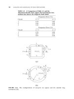
If circular symmetrical ring resonators are used with colinear feed lines,
then only one of the modes will be excited. Wolff showed that if the coupling
lines are arranged asymmetrically, as in Figure 2.3a, then both modes should
be excited [14]. The slight splitting of the resonance frequency can be easily
detected. Another way of exciting the two degenerate modes is to disturb the
symmetry of the ring resonator. Wolff also demonstrated this by using a notch
in the ring, as in Figure 2.3b [14].
Frequency splitting due to degenerate modes is undesirable in dispersion
measurements. If both modes are excited due to an asymmetric circuit, the
resonant frequency may be less distinct. To eliminate this source of error, care
should be taken to ensure that the feed lines are perfectly colinear and the
ring line width is constant.
H
k
j
AJ kr BN kr n
nnf
wm
f=¢+¢
{}
0
( ) ( ) sin( )

10 ANALYSIS AND MODELING OF RING RESONATORS
FIGURE 2.3 (a) Ring with asymmetrical feed lines, and (b) ring with a notch.
2.3.3 Mode Chart for the Resonator
It has been established that the field components on the microstrip ring
resonator are E
z
, H
r
, and H
f
. The resonant modes are a solution to the
eigenequation
(2.11)
and may be denoted as TM
nml
, where n is the azimuthal mode number, m is
the root number for each n, and l = 0 because ∂/∂z = 0. Close examination of
Equation (2.11) reveals that for narrow microstrip widths, as r
l
approaches r
o
,
the equation reduces to
(2.12)
The second term of Equation (2.12) is nonzero, and therefore
(kr
o
)
2
- n

2
= 0 (2.13)
Substituting k = 2p/l
g
and rearranging yields the well-known equation
nl
g
= 2pr
o
which gives the resonances of the TM
n10
modes.
Wu and Rosenbaum presented a mode chart for the resonant frequencies
of the various TM
nm0
modes as a function of the ring line width [4]. They also
pointed out that Equation (2.11) is the same equation that must be satisfied
for the transverse electric (TE) modes in coaxial waveguides.The fields on the
microstrip ring resonator are actually the duals of the TE modes in the coaxial
waveguide.
From the mode chart of Wu and Rosenbaum, two important observations
can be made [4]. As the normalized ring width, ring width/ring radius, (w/R)
is increased, higher-order modes are excited. This occurs when the ring width
reaches half the guided wavelength, and is similar to transverse resonance on
a microstrip line. To avoid the excitation of higher-order modes, a design cri-
teria of w/R < 0.2 should be observed. The other observation is the increase
of dispersion on narrow rings. If rings for which w/R < 0.2 are used, then dis-
persion becomes important for the modes of n > 4. Wide rings do not suffer
the effects of dispersion as much as narrow rings.
2.3.4 Improvement of the Magnetic-Wall Model

The magnetic-wall model is a nonrigorous but reasonable solution to the cur-
vature problem in the microstrip ring resonator. The main criticism of the
model is that it does not take into account the fringing fields of the microstrip
() ()() ()()kr n J kr N kr N kr J kr
onononono
22
11
0-
[]
-
{}
=

¢
()
¢
()
-¢
()
¢
()
=JkrNkr JkrNkr
noni nino
0
FIELD ANALYSES 11
line. In an attempt to take this into account, the substrate relative permittiv-
ity is made equal to the frequency-dependent effective relative permittivity,
e
eff
(f ), while retaining the same line width, w. Owens argued that this increases

the discrepancy between the quasi-static properties of the model and the
microstrip ring that it represents [2]. He further argued that dispersion char-
acteristics obtained in this way were still curvature-dependent. He proposed
to correct this inconsistency by using the planar waveguide model for the
microstrip line.
The planar waveguide model is similar to the magnetic-wall model of the
ring resonator. In this model the width of the parallel conducting plates, w
eff
(f ),
is a function of frequency (see Fig. 2.4). The separation between the plates
is equal to the distance between the microstrip line and its ground plane.
Magnetic walls enclose the substrate with a permittivity of e
eff
. The following
equations are used to calculate the effective line width:
(2.14)
where
(2.15)
and
(2.16)
where h is the substrate thickness, Z
0
is the characteristic impedance, h
0
is the
free space impedance, and c is the speed of light in a vacuum [15, 16].
To apply the planar waveguide model to the ring resonator, the inner and
outer radii of the ring, r
i
and r

o
, respectively, are compensated to give
(2.17)
Rrrwf
ooi
=+
()
+
()
[]
1
2
eff
f
c
w
p
=
eff eff
() ()00e
w
h
Z
eff
eff
()
()
0
0
0

0
=
h
e
wff w
ww
ff
p
eff
eff
()
()
()
=+
-
+
0
1
2
12 ANALYSIS AND MODELING OF RING RESONATORS
FIGURE 2.4 (a) Microstrip line and its electric fields, and (b) the planar waveguide
model of a microstrip line.
(2.18)
where R
o
and R
i
are the radii using the new model. To find the resonant fre-
quencies of the structure, solve for the eigenvalues of Equation (2.11).
Experimental results for this model compare quite accurately with known

theoretical results. The results obtained for e
eff
were not curvature dependent
as in the other models.
2.3.5 Simplified Eigenequation
The eigenequation for the magnetic-wall model can be solved numerically to
determine the resonant frequency of a given circuit. The numerical solution is
a tedious and time-consuming process that would make implementation
into CAD inefficient. Therefore closed-form expressions for the technically
interesting modes have been derived by Khilla [17]. The solution is as
follows:
For the TM
n10
modes
(2.19)
For the TM
010
mode and 0.5 < X £ 1
(2.20)
where
and w
eff
, R
o
, and R
i
are calculated from Equations (2.14), (2.17), and (2.18),
respectively. The constants A1
n
, A2

n
, A3
n
, B1
n
, B2
n
, B3
n
, and B4
n
are given in
Table 2.1. The accuracy is reported within ±0.4%.
R
RR
e
io
=
+()
2
a
p
=
-()1
2
X
X
w
R
e

=
05.
eff
kR X
e
=-+
()
1 9159 1
0 0847 0 3312
175
.
(
tan
)
tan

.
aa
kR A A
X
X
X
X
AX
enn
B
B
B
B
n

n
n
n
n
=+
()
-
+-12
2
1
31
1
2
3
4
(sin ) (cos )
()
()
pp
Rrrwf
ioi
=+
()
-
()
[]
1
2
eff
FIELD ANALYSES 13

TABLE 2.1 Constants for the Simplified Eigenequation
nA1
n
A2
n
A3
n
B1
n
B2
n
B3
n
B4
n
1 0.9206 0.0493 0.0794 -0.4129 -1.0773 5.9931 4.5168
2 1.5271 1.42E - 4 0.4729 6.3852 5.6221 -1.9139 3.8091
3 2.1005 4.42E - 6 0.8995 10.6240 9.6195 -8.3029 1.8957
2.3.6 A Rigorous Solution
The magnetic-wall model is a nonrigorous method of analysis for the ring
resonator. This method requires that either a frequency-dependent e
eff
or a
frequency-dependent line width be used to describe the edge effects.
This method adequately predicts the resonant frequency of not only the
dominant modes but also higher-order modes; beyond this is may have limited
applicability.
A rigorous solution based on the variational or stationary principle was
developed by Pintzos and Pregla in 1978 [3]. A stationary expression was
established for the resonant frequency of the dominant mode by means of the

“reaction concept” of electromagnetic theory [18]. The reaction of a field E
a
,
H
a
, on a source J
b
, M
b
in a volume V is defined as
(2.21)
In the case of a resonant structure, the self-reaction ·a, aÒ, the reaction of a
field on its own source, is zero because the true field at resonance is source-
free [19].
An approximate expression for the self-reaction can be derived using a trial
field and source. By equating this to the correct reaction, a stationary formula
for the resonant frequency can be obtained [19]. The only source is the trial
current J
s
on the microstrip line. The field associated with such a current can
be considered a trial field as well. The self-reaction can now be defined as
(2.22)
Solving Equation (2.22) is the emphasis of the approach.
The fields existing in the structure can be expressed in terms of the vector
potentials A = u
z
Y
E
and F = u
z

Y
H
by means of the following relations:
(2.23)
(2.24)
The scalar potentials Y
E
, Y
H
satisfy the Helmholtz equation
(2.25)
(2.26)
and
k
i
2
= k
0
2
e
ri
, (2.27)
—+ =YY
H
i
H
k
2
0
—+ =YY

E
i
E
k
2
0
HA F=-—¥ + —¥—¥
1
j
w
m
EF A=-—¥ + —¥—¥
1
jwe
aa dV, =◊ =
Ú
EJ
tr tr
n
0
ab dV
ab a b
,( )=◊-◊
Ú
EJ HM
n
14 ANALYSIS AND MODELING OF RING RESONATORS
where i = 1, 2 and designates the subregions 1 (substrate) and 2 (air).
The solution of Equations (2.23) and (2.24) can be represented in the form
of the Fourier–Bessel integrals for each region:

In the dielectric
(2.28)
(2.29)
In the air
(2.30)
(2.31)
where
r
i
2
+ k
0
2
e
ri
= k
r
2
(2.32)
By applying the boundary conditions at the interface z = t, the coefficients A
n
,
B
n
, C
n
, and D
n
can be determined. The continuity boundary conditions are as
follows:

E
r,1
= E
r,2
E
f,1
= E
f,2
H
r,1
- H
r,2
=-I
f
(r,f)
H
f,1
- H
f,2
=-I
f
(r,f)
where I
r
(r, f) and I
f
(r, f) are the components of the sheet current density J
tr
in the r and f directions, respectively.
After the coefficients A

n
, B
n
, C
n
, and D
n
are expressed in terms of the trial
current distribution on the surface, the expression for E
tr
can be formed from
Equation (2.23). Equation (2.22) can then be solved for the solution. Because
the r component of the current is usually small when compared to the f
current component, it can be neglected. This results in
(2.33)
for the stationary expression. This can be solved to determine the resonant
frequency of the structure. Although many steps were omitted in the proce-
dure explanation, the general idea of the method is presented.
Because this is a variational method, a crude approximation to the current
distribution can be made. The trial fields due to this trial current distribution
aa E z tI d
i
,(,)()
,
== =
•
Ú
ff
rrrr
0

0
Y
E
nDke kJkdk
n
zt
n
=
()

•
Ú
cos ( ) ( )
()
fr
r
g
rr r
2
0
Y
E
nCke kJkdk
n
zt
n
=
()

•

Ú
sin ( ) ( )
()
fr
r
g
rr r
2
0
Y
H
nBk zkJkdk
nn
=
()
•
Ú
cos ( )sinh( ) ( )fgr
rrrr1
0
Y
E
nAk zkJkdk
nn
=
()
•
Ú
sin ( )cosh( ) ( )fgr
rrrr1

0
FIELD ANALYSES 15