Microwave Ring Circuits and Related Structures phần 5 doc

where w
0
is the angular resonant frequency, U is the stored energy per cycle,
and W is the average power lost per cycle. The three main losses associated
with microstrip circuits are conductor losses, dielectric losses, and radiation
losses. The total Q-factor, Q
0
, can be expressed as
(6.11)
where Q
c
, Q
d
, and Q
r
are the individual Q-values associated with the conduc-
tor, dielectric, and radiation losses, respectively [14].
For ring and linear resonators of the same length, the dielectric and
conductor losses are equal and therefore Q
c
and Q
d
are equal.The power radi-
ated, W
r
, is higher for the linear resonator. This results in a lower Q
r
for
the linear resonator relative to the ring. We can conclude that because Q
c
and

Q
d
are equal for the two resonators, and that Q
r
is higher for the ring, that the
ring resonator has a higher Q
0
.
The unloaded Q, Q
0
, can also be determined by measuring the loaded Q-
factor, Q
L
, and the insertion loss of the ring at resonance. Figure 6.3 shows a
typical resonator frequency response. The loaded Q of the resonator is
(6.12)
where w
0
is the angular resonant frequency and w
1
- w
2
is the 3-dB bandwidth.
Normally a high Q
L
is desired for microstrip measurements. A high Q
L
requires a narrow 3-dB bandwidth, and thus a sharper peak in the frequency
response. This makes the resonant frequency more easily determined.
The unloaded Q-factor can be calculated from

Q
L
=
-
w
ww
0
12
1111
0
QQQQ
cdr
=++
DISPERSION, DIELECTRIC CONSTANT, AND Q-FACTOR MEASUREMENTS 143
FIGURE 6.3 Resonator frequency response.
(6.13)
where L is the insertion loss in dB of the ring at resonance [2]. Because the
ring resonator has a higher Q
0
and lower insertion loss than the linear res-
onator, it will also have a higher loaded Q, Q
L
. Therefore the ring resonator
has a smaller 3-dB bandwidth and sharper resonance than the linear resonator.
This also makes the ring more desirable for microstrip measurements.
Troughton recognized the disadvantages associated with using the linear
resonators for measurements and introduced the ring resonator in 1969 [1].
He proposed that the unknown effects of either open- or short-circuit cavity
terminations could be avoided by using the ring in dispersion measurements.
The equation to be used to calculate dispersion can be found by combining

Equations (6.1) and (6.4) to yield
(6.14)
Any ill effect introduced by the ring that might falsify the measured value
of wavelength or dispersion can be reduced by correctly designing the circuit.
There are five sources of error that must be considered:
a. Because the transmission line has a curvature, the dispersion on the ring
may not be equal to the straight-line dispersion.
b. Field interactions across the ring could cause mutual inductance.
c. The assumption that the total effective length of the ring can be calcu-
lated from the mean radius.
d. The coupling gap may cause field perturbations on the ring.
e. Nonuniformities of the ring width could cause resonance splitting.
To minimize problems (a) through (d) only rings with large diameters
should be used. Troughton used rings that were five wavelengths long at the
frequency of interest. A larger ring will result in a larger radius of curvature
and thus approach the straight-line approximation and diminish the effect of
(a). The large ring will reduce (b) and the effect of (d) will be minimized
because the coupling gap occupies a smaller percentage of the total ring. The
effect of the mean radius, (c), can be reduced by using large rings and narrow
line widths.
An increased ring diameter will also increase the chance of variations in the
line width, and the possibility of resonance splitting is increased. The only way
to avoid resonance splitting is to use precision circuit processing techniques.
Troughton used another method to diminish the effect of the coupling gap.
An initial gap of 1 mil was designed. Using swept frequency techniques, Q-
factor measurements were made. The gap was etched back until it was obvious
that the coupling gap was not affecting the frequency.
e
p
eff

f
nc
fr
()
=
Ê
Ë
ˆ
¯
2
2
Q
Q
L
L
0
20
110
=
-
()
-
144 MEASUREMENT APPLICATIONS USING RING RESONATORS
The steps Troughton used to measure dispersion can be summarized as
follows:
1. Design the ring at least five wavelengths long at the lower frequency of
interest.
2. Minimize the effect of the coupling gap by observing the Q-factor and
etching back the gap when necessary.
3. Measure the resonant frequency of each mode.

4. Apply Equation (6.4) to calculate e
eff
.
5. Plot e
eff
versus frequency.
This technique was very important when it was introduced because of the
very early stage that the microstrip transmission line was in. Because it was in
its early stage, there had been little research that resulted in closed-form
expressions for designing microstrip circuits. This technique allowed the fre-
quency dependency of e
eff
to be quickly measured and the use of microstrip
could be extended to higher frequencies more accurately.
6.3 DISCONTINUITY MEASUREMENTS
One of the most interesting applications of the ring is its use to characterize
equivalent circuit parameters of microstrip discontinuities [3, 12]. Because
discontinuity parameters are usually very small, extreme accuracy is needed
and can be obtained with the ring resonator.
The main difficulty in measuring the circuit parameters of microstrip dis-
continuities resides in the elimination of systematic errors introduced by the
coaxial-to-microstrip transitions. This problem can be avoided by testing dis-
continuities in a resonant microstrip ring that may be loosely coupled to test
equipment. The resonant frequency for narrow rings can be approximated
fairly accurately by assuming that the structure resonates if its electrical length
is an integral multiple of the guided wavelength. When a discontinuity is intro-
duced into the ring, the electric length may not be equal to the physical length.
This difference in the electric and physical length will cause a shift in the res-
onant frequency. By relating the Z-parameters of the introduced discontinu-
ity to the shift in the resonance frequency the equivalent circuit parameters

of the discontinuity can be evaluated.
It has also been explained that the TM
n10
modes of the microstrip ring are
degenerate modes.When a discontinuity is introduced into the ring, the degen-
erate modes will split into two distinct modes. This splitting can be expressed
in terms of an even and an odd incidence on the discontinuity. The even case
corresponds to the incidence of two waves of equal magnitude and phase. In
the odd case, waves of equal magnitude but opposite phase are incident from
both sides. Either mode, odd or even, can be excited or suppressed by an
appropriate choice of the point of excitation around the ring.
DISCONTINUITY MEASUREMENTS 145
A symmetrical discontinuity can be represented by its T equivalent circuit
expressed in terms of its Z-parameters. The T equivalent circuit is presented
in Figure 6.4. For convenience the circuit is divided into two identical half-
sections of zero electrical length. If this circuit is excited in the even mode, it
is as if there is an open circuit at the plane of reference z = 0. The normalized
even input impedance at either port is thus Z
ie
= Z
11
+ Z
12
(see Figure 6.5a).
If this circuit is excited in the odd mode, it is as if there is a short circuit at the
plane z = 0. The normalized odd input impedance is thus Z
io
= Z
11
- Z

12
(see
Figure 6.5b). If the discontinuity is lossless, only the resonance frequencies of
the perturbed ring are affected since the even and odd impedances are purely
reactive. The artificial increase or decrease of the electrical length of the ring,
resulting in the decrease of its resonance frequencies, is related to the even
and odd impedances by the following expressions:
(6.15)
(6.16)
ZZZ jkl
io o
=-=
11 12
tan
ZZZ jkl
ie e
=+=-
11 12
cot
146 MEASUREMENT APPLICATIONS USING RING RESONATORS
FIGURE 6.4 T equivalent circuit of a discontinuity expressed in terms of its
Z-parameters.
FIGURE 6.5 (a) Impedance of a discontinuity with an even-mode incidence, and (b)
the impedance of a discontinuity with an odd-mode incidence.
where k = 2p/l
g
is the propagation constant, and l
e
and l
o

are the artificial
electrical lengths introduced by the even and odd discontinuity impedances.
Since at resonance the total electrical length of the resonator is nl
g
, the
resonance conditions are, in the even case,
(6.17)
and in the odd case,
(6.18)
where l
ring
is the physical length of the ring, and l
ge
and l
go
are the guided wave-
lengths to the even and odd resonance frequency, respectively. Since l
ring
is
known and l
g
can be obtained from measurements, l
e
and l
o
can be determined
from Equations (6.17) and (6.18). The parameters Z
11
and Z
12

can be deter-
mined by substituting Equations (6.17) and (6.18) into Equations (6.15) and
(6.16) to yield [3]
(6.19)
(6.20)
where l
g
was replaced by
and f
re
and f
ro
are the measured odd and even resonant frequencies of the
perturbed ring.
The procedure described can be altered slightly and used to evaluate lossy
discontinuities. Instead of the even an odd modes having open or short
circuits at the plane of reference, z = 0, there is introduced a termination
resistance. The termination resistance can be determined by measuring the
circuit Q-factor.
6.4 MEASUREMENTS USING FORCED MODES OR SPLIT MODES
As shown earlier, the guided wavelength of the regular mode can be easily
obtained from physical dimensions. Because of this advantage, the regular
mode has been widely used to measure the characteristics of microstrip
line. The forced modes and split modes, however, can also be applied for such
measurements [15].
l
e
g
c
ff

=
()
eff
ZZ j
lff
c
ro ro
11 12
-=-
()
tan
pe
ring eff
ZZ j
lff
c
re re
11 12
+=
()
cot
pe
ring eff
lln
og
o
ring
+=2 l
lln
egering

+=2 l
MEASUREMENTS USING FORCED MODES OR SPLIT MODES 147
6.4.1 Measurements Using Forced Modes
The forced mode phenomenon was studied previously in Chapter 3. The
shorted forced mode, as illustrated in Figure 6.6 with shorted boundary
condition at 90°, is now used to measure the effective dielectric constant of
microstrip line. The standing-wave patterns of this circuit is shown in Figure
6.7. According to the design rule mentioned in Chapter 3, the shorted forced
modes contains full-wavelength resonant modes with odd integer mode
numbers and excited half-wavelength modes with mode number n = (2m ± 1)/2,
where m = 1,3,5, The guided wavelength of each resonant mode can be
calculated by applying Equation (6.1). The resonant frequencies of each res-
148 MEASUREMENT APPLICATIONS USING RING RESONATORS
FIGURE 6.6 Coupled annular circuit with short plane at q
ss
= 90°.
FIGURE 6.7 Standing wave patterns of the shorted forced mode.
MEASUREMENTS USING FORCED MODES OR SPLIT MODES 149
FIGURE 6.8 Effective dielectric constants vs. resonant frequency for the forced mode
and regular mode.
onant mode can be measured with an HP8510 network analyzer.The effective
dielectric constants for the different resonant frequencies are determined by
the following equation:
(6.21)
where l
0
is the wavelength in free space and l
g
is the guided wavelength.
Figure 6.8 displays the effective dielectric constants versus frequency that were

calculated by the forced mode and regular mode. A comparison of these two
results shows that the excited half-wavelength resonant modes have higher
dielectric constants than the full-wavelength modes. This phenomenon reveals
that the excited half-wavelength modes travel more slowly than the full-
wavelength modes inside the annular element.
6.4.2 Measurements Using Split Modes
The idea of using the split mode for dispersion measurement was introduced
by Wolff [16]. He used notch perturbation for the measurement and found that
the frequency splitting depended on the depth of the notch. The experimen-
tal maximum splitting frequency was 53MHz. Instead of using the notch
ell
eff
=
()
0
2
g
perturbation, the local resonant split mode is developed to do the dispersion
measurement. As illustrated in Figure 6.9, a 60° local resonant sector (LRS)
was designed on the symmetric coupled annular ring circuit. The test circuit
was built on a RT/Duroid 6010.5 substrate with the following dimensions:
150 MEASUREMENT APPLICATIONS USING RING RESONATORS
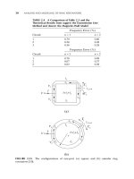
FIGURE 6.9 Layout of annular circuit with 60° LRS resonant sector.
FIGURE 6.10 |S
21
| vs. frequency for the first six resonant modes of Figure 6.9.
MEASUREMENTS USING FORCED MODES OR SPLIT MODES 151
FIGURE 6.11 Splitting frequency vs. width of the 60° LRS.
According to the analysis in Chapter 3, the resonant modes with mode
number n = 3 m, where m = 1,2,3, ,will not split. Figure 6.10 illustrates the

nondisturbed third and sixth resonant modes and the other four split resonant
modes that agree with the prediction of standing-wave pattern analysis.
By increasing the perturbation width the frequency-splitting effect will
become larger. Figure 6.11 displays the experimental results of the depend-
ence of splitting frequency on the width of the LRS. The largest splitting fre-
quency shown in Figure 6.11 is 765 MHz for the LRS with 3.5 mm width. The
use of the local resonant split mode is more flexible than the notch perturba-
tion. The local resonant split mode can also be applied to the measurements
of step discontinuities of microstrip lines [17].
Substrate thickness = 0.635mm
Line width = 0.6mm
LRS line width = 1.1mm
Coupling gap = 0.1mm
Ring radius = 6mm
REFERENCES
[1] P. Troughton, “Measurement technique in microstrip,” Electron. Lett., Vol. 5, No.
2, pp. 25–26, January 23, 1969.
[2] K. Chang, F. Hsu, J. Berenz, and K. Nakano, “Find optimum substrate thickness
for millimeter-wave GaAs MMICs,” Microwaves & RF, Vol. 27, pp. 123–128,
September 1984.
[3] W. Hoefer and A. Chattopadhyay, “Evaluation of the equivalent circuit parame-
ters of microstrip discontinuities through perturbation of a resonant ring,” IEEE
Trans. Microwave Theory Tech., Vol. MTT-23, pp. 1067–1071, December 1975.
[4] T. C. Edwards, Foundations for Microstrip Circuit Design, Wiley, Chichester,
England, 1981; 2d ed., 1992.
[5] J. Deutsch and J. J. Jung, “Microstrip ring resonator and dispersion measurement
on microstrip lines from 2 to 12 GHz,” Nachrichtentech. Z., Vol. 20, pp. 620–624,
1970.
[6] I. Wolff and N. Knoppik, “Microstrip ring resonator and dispersion measurements
on microstrip lines,” Electron. Lett.,Vol. 7, No. 26, pp. 779–781, December 30, 1971.

[7] H. J. Finlay, R. H. Jansen, J. A. Jenkins, and I. G. Eddison, “Accurate characteriza-
tion and modeling of transmission lines for GaAs MMICs,” in 1986 IEEE MTT-
S Int. Microwave Symp. Dig., New York, pp. 267–270, June 1986.
[8] P. A. Bernard and J. M. Gautray, “Measurement of relative dielectric constant
using a microstrip ring resonator,” IEEE Trans. Microwave Theory Tech., Vol.
MTT-39, pp. 592–595, March 1991.
[9] P. A. Polakos, C. E. Rice, M. V. Schneider, and R. Trambarulo, “Electrical
characteristics of thin-film Ba
2
YCu
3
O
7
superconducting ring resonators” IEEE
Microwave Guided Wave Lett., Vol. 1, No. 3, pp. 54–56, March 1991.
[10] M. E. Goldfarb and A. Platzker, “Losses in GaAs Microstrip,” IEEE Trans.
Microwave Theory Tech., Vol. MTT-38, No. 12, pp. 1957–1963, December 1990.
[11] S. Kanamaluru, M. Li, J. M. Carroll, J. M. Phillips, D. G. Naugle, and K. Chang,
“Slotline ring resonator test method for high-Tc superconducting films,” IEEE
Trans. App. Supercond., Vol. ASC-4, No. 3, pp. 183–187, September 1994.
[12] T. S. Martin, “A study of the microstrip ring resonator and its applications,” M.S.
thesis, Texas A&M University, College Station, December 1987.
[13] P. Troughton, “High Q-factor resonator in microstrip,” Electron. Lett., Vol. 4, No.
24, pp. 520–522, November 20, 1968.
[14] E. Belohoubek and E. Denlinger, “Loss considerations for microstrip resonators,”
IEEE Trans. Microwave Theory Tech., Vol. MTT-23, pp. 522–526, June 1975.
[15] C. Ho and K. Chang, “Mode phenomenons of the perturbed annular ring ele-
ments,” Texas A&M University Report, College Station, September 1991.
[16] I. Wolff, “Microstrip bandpass filter using degenerate modes of a microstrip ring
resonator,” Electron. Lett., Vol. 8, No. 12, pp. 302–303, June 15, 1972.

[17] K. C. Gupta, R. Garg, and I. J. Bahl, Microstrip Lines and Slotlines, Artech House,
Dedham, Mass., pp. 189–192, 1979.
152
MEASUREMENT APPLICATIONS USING RING RESONATORS
CHAPTER SEVEN
Filter Applications
7.1 INTRODUCTION
As shown in the previous chapters, the ring resonator has bandpass charac-
teristics. If a ring resonator is coupled to input and output transmission lines,
the signal will pass through with certain losses at the resonant frequencies of
the ring and will be rejected at frequencies outside the resonant frequencies.
By cascading several ring resonators in series, various bandpass filtering char-
acteristics can be designed.As discussed in Chapters 2 and 3, the ring resonator
can support two degenerate modes if both modes are excited. This forms the
base for a compact dual-mode filter. The ring resonators could be designed in
microstrip line, slotline, or coplanar waveguide. The ring cavities can be built
in waveguides.
7.2 DUAL-MODE RING BANDPASS FILTERS
As described in Chapters 2 and 3, the dual-mode effects are introduced either
by skewing one of the feed lines with respect to the other or by introduction
of a discontinuity (notch, slit, patch, etc.). The dual-mode bandpass filter was
first proposed by Wolff using asymmetric coupling feed lines [1]. Later on,
many new configurations using orthogonal feed lines with patch perturbation
on a ring resonator were introduced [2–5]. The new configuration with orthog-
onal feed lines and patch perturbation provides a quasi-elliptic function that
has two transmission zeros close to the passband. This property can be used
to reject adjacent channel interferences.
Figure 7.1 shows a dual-mode filter. The square ring resonator is fed by a
153
Microwave Ring Circuits and Related Structures, Second Edition,

by Kai Chang and Lung-Hwa Hsieh
ISBN 0-471-44474-X Copyright © 2004 John Wiley & Sons, Inc.
pair of orthogonal feed lines, and each feed line is connected to an L-shape
coupling arm [6]. Figure 7.1b displays the scheme of the coupling arm that con-
sists of a coupling stub and a tuning stub. The tuning stub attached to the end
of the coupling stub extends the coupling stub to increase the coupling periph-
ery. In addition, the asymmetrical structure perturbs the field of the ring res-
onator and excites two degenerate modes [1]. Without the tuning stubs, there
is no perturbation on the ring resonator and only a single mode is excited [7].
Comparing the filter in Figure 7.1 with conventional dual-mode filters [1], the
conventional filters only provide a dual-mode characteristic without the ben-
efits of enhanced coupling strength and performance optimization.
The filter was designed at the center frequency of 1.75GHz and fabricated
154 FILTER APPLICATIONS
l
f
l
c
l
t
g
l
s
w
Feed line
Tuning
stub
Coupling stub
(b)
(a)

FIGURE 7.1 Dual-mode bandpass filter with enhanced coupling (a) layout and (b)
L-shape coupling arm [6]. (Permission from IEEE.)
on a 50-mil thickness RT/Duroid 6010.2 substrate with a relative dielectric
constant of 10.2. The length of the tuning stubs is l
t
, and the gap size between
the tuning stubs and the ring resonator is s. The length of the feed lines is l
f
=
8 mm; the width of the microstrip line is w = 1.191 mm for a 50-ohm line; the
length of the coupling stubs is l
c
= 18.839 + smm; the gap size between the ring
resonator and coupling stubs is g = 0.25 mm; the length of one side of the
square ring resonator is l = 17.648mm. The coupling gap g was selected in con-
sideration of strong coupling and etching tolerance. The simulation was com-
pleted using an IE3D electromagnetic simulator [8].
By adjusting the length l
t
and gap size s of the tuning stubs adequately, the
coupling strength and the frequency response can be optimized. Single-mode
excitation (Figure 7.2) or dual-mode excitation (Figure 7.3) can be resulted by
varying s and l
t
. Figures 7.2 and 7.3 show the measured results for five cases
from changing the length l
t
of tuning stubs with a fixed gap size (s = 0.8 mm)
and varying the gap size s with a fixed length (l
t

= 13.5 mm). Observing the
measured results in Figure 7.2, two cases for l
t
= 4.5 and 9 mm with a fixed gap
size only excite a single mode.
The coupling between the L arms and the ring can be expressed by exter-
nal Q (Q
e
) as follows [9]:
(7.1a)
(7.1b)
where Q
L
is the loaded Q, Q
o
is the unloaded Q of the ring resonator, f
o
is the
resonant frequency, (Df)
3dB
is the 3-dB bandwidth, and L is the insertion loss
in decibel. The loaded Q is obtained from measurement of f
o
and (Df)
3dB
and
unloaded Q (Q
o
= 137) is calculated from the Equation (7.1b). From Equation
(7.1a), Q

e
is given by
(7.2)
The performance for these two single-mode ring resonators is shown in Table
7.1.
The coupling coefficient between two degenerate modes is given by [10]
(7.3)
K
ff
ff
pp
pp
=
-
+
21
21
22
22
Q
QQ
QQ
e
oL
oL
=
-
2
Q
Q

o
L
L
=
-
()
-
110
20
Q
QQ
f
f
L
eo
o
dB
=
+
=
()
1
21
3
D
DUAL-MODE RING BANDPASS FILTERS 155
where f
p1
and f
p2

are the resonant frequencies. In addition, the midband inser-
tion loss L corresponding to Q
o
, Q
e
, and K can be expressed as [9]
(7.4)
L
QQ
KQ
KQ
eo
e
e
=
+
()
+
È
Î
Í
˘
˚
˙
20
1
22
2
log dB
156 FILTER APPLICATIONS

1.0 1.5 2.0 2.5 3.0
Frequency (GHz)
-80
-60
-40
-20
0
Magnitude (dB)
S
21
l
t
= 4.5 mm,
Q
e
= 61.16
l
t
= 9 mm,
Q
e
= 25.58
(a)
l
t
= 4.5 mm,
Q
e
= 61.16
l

t
= 9 mm,
Q
e
= 25.58
1.0 1.5 2.0 2.5 3.0
Frequency (GHz)
-25
-20
-15
-10
-5
0
Magnitude (dB)
S
11
(b)
FIGURE 7.2 Measured (a) S
21
and (b) S
11
by adjusting the length of the tuning stub
l
t
with a fixed gap size (s = 0.8 mm) [6]. (Permission from IEEE.)
DUAL-MODE RING BANDPASS FILTERS 157
1.0 1.5 2.0 2.5 3.0
Frequency (GHz)
-80
-60

-40
-20
0
Magnitude (dB)
S
21
s
= 0.3 mm,
Q
e
= 6.24,
K
= 0.075
s
= 0.5 mm,
Q
e
= 7.9,
K
= 0.078
s
= 0.8 mm,
Q
e
= 9.66,
K
= 0.08
(a)
s
= 0.3 mm,

Q
e
= 6.24,
K
= 0.075
s
= 0.5 mm,
Q
e
= 7.9,
K
= 0.078
s
= 0.8 mm,
Q
e
= 9.66,
K
= 0.08
1.0 1.5 2.0 2.5 3.0
Frequency (GHz)
-30
-20
-10
0
Magnitude (dB)
S
11
(b)
FIGURE 7.3 Measured (a) S

21
and (b) S
11
by varying the gap size s with a fixed length
of the tuning stubs (l
t
= 13.5 mm) [6]. (Permission from IEEE.)
TABLE 7.1 Single-Mode Ring Resonator [6]. (Permission from IEEE.)
Case l: l
l
= 4.5 mm Case 2: l
l
= 9mm
s = 0.8 mm s = 0.8 mm
Resonant Frequency f
o
1.75 GHz 1.755 GHz
Insertion Loss IL 2.69 dB 0.97 dB
3-dB Bandwidth 70 MHz 150 MHz
Loaded Q 25 11.7
External Q 61.16 25.58
The external Q can be obtained from Equation (7.4) through measured L, K,
and Q
o
. Moreover, the coupling coefficient between two degenerate modes
shows three different coupling conditions.
(7.5)
If the coupling coefficient satisfies K > K
o
, then the coupling between two

degenerate modes is overcoupled. In this overcoupled condition, the ring res-
onator has a hump response with a high insertion loss in the middle of the
passband [5]. If K = K
o
, the coupling is critically coupled. Finally, if K < K
o
, the
coupling is undercoupled. For both critically coupled and undercoupled cou-
pling conditions, there is no hump response. Also, when the coupling becomes
more undercoupled, the insertion loss in the passband increases [9]. The per-
formance for the dual-mode ring resonators is displayed in Table 7.2.
Observing the single-mode ring in Table 7.1, it shows that a higher external
Q produces higher insertion loss and narrower bandwidth. In addition, for the
dual-mode ring resonator in Table 7.2, its insertion loss and bandwidth depend
on the external Q, coupling coefficient K, and coupling conditions. For an
undercoupled condition, the more undercoupled, the more the insertion loss
and the narrower the bandwidth.To obtain a low insertion-loss and wide-band
pass band characteristic, the single-mode ring resonator should have a low
external Q, which implies more coupling periphery between the feeders and
the ring resonator.
Figure 7.4 shows the simulated and measured results for the optimized
quasi-elliptic bandpass filter. Two transmission zeros locate on either side of
the passband to suppress unwanted adjacent channel interferences. The filter
has an insertion loss of 1.04 dB in the passpband with a 3-dB bandwidth of
192.5 MHz.
Let KQQ
oeo
=+11.
158 FILTER APPLICATIONS
TABLE 7.2 Dual-Mode Ring Resonator [6]. (Permission from IEEE.)

Case l: Case 2: Case 3:
l
l
= 13.5 mm l
l
= 13.5 mm l
l
= 13.5 mm
s = 0.3 mm s = 0.5 mm s = 0.8 mm
Resonant Frequencies (1.72, 1.855) GHz (1.7, 1.84) GHz (1.67, 1.81) GHz
(f
p1
, f
p2
)
Coupling Coefficient 0.075 0.078 0.08
K
External Q 6.24 7.9 9.66
Midband Insertion 2.9 dB 1.63 dB 1.04 dB
Loss IL
3-dB Bandwidth 160 MHz 175 MHz 192.5 MHz
Coupling Condition undercoupled undercoupled undercoupled
Cascaded multiple ring resonators have advantages in acquiring a much
narrower and shaper rejection. Figure 7.5 illustrates the filter using three cas-
caded ring resonators. Any two of three resonators are linked by an L-shape
arm with a short transmission line l
e
of 6.2 mm with a width w
1
= 1.691mm.

DUAL-MODE RING BANDPASS FILTERS 159
S
11
S
21
1.0 1.5 2.0 2.5 3.0
Frequency (GHz)
-80
-60
-40
-20
0
Magnitude (dB)
Measurement
Simulation
FIGURE 7.4 Simulate and measured results for the case of l
t
= 13.5 mm and s =
0.8 mm [6]. (Permission from IEEE.)
w
w
1
l
e
w
l
e
w
1
FIGURE 7.5 Layout of the filter using three resonators with L-shape coupling arms

[6]. (Permission from IEEE.)
This bandpass filter was built based on the l
t
= 13.5 mm and s = 0.8 mm case
of the single ring resonator of Figure 7.1. Each filter section has identical
dimensions as that in Figure 7.1. The energy transfers from one ring resonator
through the coupling and tuning stubs (or an L-shape arm) and the short trans-
mission line to another ring resonator. Observing the configuration for the L-
shape and the short transmission line l
e
in Figure 7.6, it not only perturbs the
ring resonator, but also it can be treated as a resonator. A short transmission
line l
c
of 6.2 mm with a width w
1
= 1.691 mm connects to the coupling stubs to
link the two ring resonators.
Considering this type resonator in Figure 7.6a, it is consisted of a transmis-
sion line l
e
and two parallel-connected open stubs. Its equivalent circuit is
shown in Figure 7.6b. The input admittance Y
in
is given by
Y
in1
= jY
o
[tan(bl

a
) + tan(bl
a
)], b: phase constant
Y
l
= 1/Z
l
, Y
o
= 1/Z
o
. (7.6)
Y
1
is the characteristic admittance of the transmission line l
e
, and Y
o
is the
characteristic admittances of the transmission lines l
a
, and l
b
. Letting Y
in
= 0,
the resonant frequencies of the resonator can be predicted. The resonant fre-
YY Y
YjY l

YjY l
in in
in e
in e
=+
+
()
+
()
È
Î
Í
˘
˚
˙
11
11
11
tan
tan
b
b
160 FILTER APPLICATIONS
w
1
l
e
Y
in
w

Open End
Effect
l
a
l
b
(a)
Y
in
Y
in1
Y
in1
Z
1
l
e
(b)
FIGURE 7.6 Back-to-back L-shape resonator (a) layout and (b) equivalent circuit.
The lengths l
a
and l
b
include the open end effects.
quencies of the resonator are calculated as f
o1
= 1.067, f
o2
= 1.654, and f
o3

=
2.424 GHz within 1–3 GHz. To verify the resonant frequencies, an end-to-side
coupling circuit is built as shown in Figure 7.7.
Also, the measured resonant frequencies can be found as f
mo1
= 1.08, f
mo2
=
1.655, and f
mo3
= 2.43 GHz, which show a good agreement with calculated
results. Inspecting the frequency responses in Figures 7.6 and 7.7, the spike at
f
mo3
= 2.43 GHz is suppressed by the ring resonators and only one spike appears
at low frequency ( f
mo1
= 1.08 GHz) with a high insertion loss, which dose not
influence the filter performance. Furthermore, the resonant frequency ( f
mo2
=
1.655 GHz) of the resonator in Figure 7.6 couples with the ring resonators.
By changing the length l
e
, the resonant frequencies will move to different loca-
tions. For a shorter length l
e
, the resonant frequencies move to higher fre-
quency and for a longer length l
e

, the resonant frequencies shift to lower
frequency. Considering the filter performance, a proper length l
e
should be
carefully chosen. The simulated and measured results of the three cascaded
ring filter are shown in Figure 7.8. The filter has a measured insertion loss of
2.39 dB in the passpband with a 3-dB bandwidth of 145 MHz.
7.3 RING BANDSTOP FILTERS
The bandstop characteristic of the ring circuit can be realized by using two
orthogonal feed lines with coupling gaps between the feed lines and the ring
resonator [11]. For odd-mode excitation, the output feed line is coupled to a
position of the zero electric field along the ring resonator and shows a short
RING BANDSTOP FILTERS 161
1.0 1.5 2.0 2.5 3.0
Frequency (GHz)
-110
-90
-70
-50
-30
Magnitude (dB)
S
21
FIGURE 7.7 Measured S
21
for the back-to-back L-shape resonator [6]. (Permission
from IEEE.)
circuit [12]. Therefore, no energy is extracted from the ring resonator, and the
ring circuit provides a stopband. A ring resonator directly connected to a pair
of orthogonal feed lines is shown in Figure 7.9 [13]. In this case, no coupling

gaps are used between the resonator and the feed lines for low insertion loss.
The circumference l
r
of the ring resonator is expressed as
(7.7)
where n is the mode number and l
g
is the guided wavelength. In order to inves-
tigate the behavior of this ring circuit, an EM simulator [8] and a transmission
line model are used.
ln
rg
= l
162 FILTER APPLICATIONS
S
11
S
12
3.02.52.01.51.0
Frequency (GHz)
-80
-60
-40
-20
0
Magnitude(dB)
Measurement
Simulation
FIGURE 7.8 Simulated and measured results for the filter using three resonators with
L-shape coupling arms [6]. (Permission from IEEE.)

Input
Output
l
f
l
r
= n
g
l
w
1
l
FIGURE 7.9 A ring resonator using direct-connected orthogonal feeders [12].
(Permission from IEEE.)
Figure 7.10 shows the EM simulated electric current distribution of the ring
circuit and a conventional l
g
/4 open-stub bandstop filter at the same funda-
mental resonant frequency. The arrows represent the electric current.The sim-
ulated electric current shows minimum electric fields at positions A and B,
which correspond to the maximum magnetic fields. Thus, both circuits provide
bandstop characteristics by presenting zero voltages to the outputs at the fun-
damental resonant frequency that can be observed by their simulated fre-
quency response of S
21
as shown in Figure 7.11.
The ring resonator and the conventional l
g
/4 open-stub bandstop filter are
designed at a fundamental resonant frequency of f

o
= 5.6GHz and fabricated
on a RT/Duriod 6010.2 substrate with a thickness h = 25 mil and a relative
dielectric constant e
r
= 10.2. The dimensions of the ring are l
f
= 5 mm, l
r
=
20.34 mm, and w
1
= 0.6mm.
RING BANDSTOP FILTERS 163
Input Output
B
Input
Output
A
FIGURE 7.10 Simulated electric current at the fundamental resonant frequency for
the ring and open-stub bandstop circuits [12]. (Permission from IEEE.)
0246810
Frequency (GHz)
-80
-60
-40
-20
0
Magnitude (dB)
S

21
Ring circuit
Open stub circuit
FIGURE 7.11 Simulated results for the bandstop filters [12]. (Permission from IEEE.)
The equivalent ring circuit shown in Figure 7.12 is divided by the input and
output ports to form a shunt circuit denoted by the upper and lower parts,
respectively.
The equivalent circuits of the 45-degree-mitered bend are represented by
two inductors L and a capacitor C [14] those are expressed by
(7.8a)
(7.8b)
where h and w
1
are in millimeters. The capacitance jB
T
is the T-junction effect
between the feed line and the ring resonator [15]. The frequency response of
the ring circuit can be calculated from the equivalent ring circuit using ABCD,
Y, and S parameters. Figure 7.13 shows the calculated and measured results
with good agreement.
7.4 COMPACT, LOW INSERTION LOSS, SHARP REJECTION, AND
WIDEBAND BANDPASS FILTERS
Figure 7.14 shows a compact, low insertion loss, sharp rejection, wideband
microstrip bandpass filter.This bandpass filter is developed from the bandstop
filter introduced in Section 7.3 [13]. Two tuning stubs are added to the band-
stop filter to create a wide passband.Without coupling gaps between feed lines
and rings, there are no mismatch and radiation losses between them [16].Thus,
the filter can obtain a low insertion loss, and the major losses of the filter
are contributed by conductor and dielectric losses. In Figure 7.14, the ring
resonator is loaded with two tuning stubs of length l

t
= l
g
/4 at F=90° and
Lh
w
h
=- -
Ê
Ë
ˆ
¯
È
Î
Í
˘
˚
˙
Ï
Ì
Ó
¸
˝
˛
022 1 135 018
1
139
. . exp .
.
n

H
Ch
w
h
w
h
rr
=+
()
Ê
Ë
ˆ
¯
++
Ê
Ë
ˆ
¯
È
Î
Í
˘
˚
˙
0001 339 062 76 38
1
2
1
. eepF
164 FILTER APPLICATIONS

l
f
jB
T
l
l
l
l
l
l
l
l
f
jB
T
LL
L
L
L
L
Lower part
Upper part
Input
Output
c
c
c
c
LL
l

FIGURE 7.12 Equivalent circuit of the ring using direct-connected orthogonal feed
lines [12]. (Permission from IEEE.)
COMPACT, LOW INSERTION LOSS, SHARP REJECTION, AND BANDPASS FILTERS 165
0246810
Frequency (GHz)
-80
-60
-40
-20
0
Magnitude (dB)
Measurement
Calculation
S
11
S
21
FIGURE 7.13 Calculated and measured results of the ring using direct-connected
orthogonal feed lines [12]. (Permission from IEEE.)
l
t
w
2
F
y
x
0
o
F=
Input

Output
(a)
C
C
Input
Output
l
f
jB
T
l
l
l
l
l
l
l
l
f
jB
T
L
L
L
L
Y
t
Y
t
l

C
L
L
C
L
L
(b)
FIGURE 7.14 Ring with two tuning stubs at F=90° and 0° (a) layout and (b) equiv-
alent circuit.
166 FILTER APPLICATIONS
l
t
= 1.25 mm
l
t
= 2.50 mm
l
t
= 3.75 mm
l
t
= 5.03 mm
13579111315
Frequency (GHz)
-80
-60
-40
-20
0
Magnitude (dB)

S
21
FIGURE 7.15 Calculated results of the ring with various lengths of the tuning stub at
F=90° and 0° [12]. (Permission from IEEE.)
F=0°. Y
t
is the admittance looking into the tuning stub and can be expressed
by
(7.9)
where Y
o
is the characteristic admittance of the tuning stub, b is the propaga-
tion constant, and l
open
is the equivalent open-effect length [17]. The frequency
response of the ring circuit can be obtained from the equivalent circuit by
using ABCD, Y, and S parameter calculations.
By changing the lengths of two tuning stubs, the frequency response of the
ring circuit will be varied. Observing the calculated results in Figure 7.15, two
attenuation poles starting from the center frequencies of the fundamental and
the third modes move to the lower frequencies and form a wide passband. The
measured and calculated results of the filter with the tuning stubs of length
l
g
/4 are shown in Figure 7.16. In addition, due to the symmetric structure, the
ring circuit in Figure 7.14 only excites a single mode.
Observing the results in Figure 7.16, the effects of adding two tuning
stubs with a length of l
t
= l

g
/4 at F=90° and F=0° provide a sharper cutoff
frequency response, increase attenuations, and obtain a wide passband. Two
attenuation poles are at f
1
= 3.81 GHz with -46-dB rejection and f
2
= 7.75 GHz
with -51-dB rejection. The differences between the measurement and the cal-
culation on f
1
and f
2
are due to fabrication tolerances that cause a slightly
asymmetric layout and excite small degenerate modes.
The key point behind this new filter topology is that two tuning stubs loaded
on the ring resonator at F=90° and F=0° are used to achieve a wide pass-
band with a sharp cutoff characteristic. In some cases, an undesired passband
YY ll jB
t o t open T
=+
()
[]
+tanh b
1
below the main passband may require a high passband section to be used in
conjunction with this approach.
In Figure 7.16, the two stopbands of the filter show a narrow bandwidth.To
increase the narrow stopbands, a dual-mode design can be used [4]. A square
perturbation stub at F=45° is incorporated on the ring resonator in Figure

7.17a. The square stub perturbs the fields of the ring resonator so that the res-
onator can excite a dual mode around the stopbands in order to improve the
narrow stopbands. By increasing (decreasing) the size of the square stub, the
distance (stopband bandwidth) between two modes is increased (decreased).
The equivalent circuits of the square stub and the filter are displayed in Figure
7.17b and c, respectively. As seen in Figure 7.17b, the geometry at the corner
of F=45° is approximately equal to the square section of width w
1
+ w
p,
sub-
tracting an isometric triangle of height w
1
. Also, the equivalent L-C circuit of
this approximation is shown in Figure 7.17c, where C
pf
= C
r
- C and L
p
= LL
r
/
(L - L
r
). The equivalent capacitance and inductance of the right angle bend,
C
r
and L
r

, are given by [14]
(7.10a)
(7.10b)
The asymmetric step capacitance C
s
is [18]
(7.11)
Cw
sp r
=+
()
0 012 0 0039 e pF
Lh
ww
h
p
=- -
+
Ê
Ë
ˆ
¯
È
Î
Í
˘
˚
˙
Ï
Ì

Ó
¸
˝
˛
022 1 135 018
1
139
. . exp .
.
nH
Ch
ww
h
ww
h
rr
p
r
p
=+
()
+
Ê
Ë
ˆ
¯
++
+
Ê
Ë

ˆ
¯
È
Î
Í
˘
˚
˙
0 001 10 35 2 5 2 6 5 64
1
2
1
eepF
COMPACT, LOW INSERTION LOSS, SHARP REJECTION, AND BANDPASS FILTERS 167
0246810
Frequency (GHz)
-60
-45
-30
-15
0
Magnitude (dB)
S
11
S
21
Calculation
Measurement
FIGURE 7.16 Calculated and measured results of the ring with two tuning stubs of
l

t
= l
g
/4 = 5.026 mm at F=90° and 0° [12]. (Permission from IEEE.)