Báo cáo lâm nghiệp:"Optimising the management of Scots pine (Pinus sylvestris L.) stands in Spain based on individual-tree models" potx

105
Ann. For. Sci. 60 (2003) 105–114
© INRA, EDP Sciences, 2003
DOI: 10.1051/forest:2003002
Original article
Optimising the management of Scots pine (Pinus sylvestris L.) stands
in Spain based on individual-tree models
Marc Palahí
a
* and Timo Pukkala
b

a
European Forest Institute, Torikatu 34, 80100 Joensuu, Finland
b
University of Joensuu, Faculty of Forestry, PO Box 111, 80101 Joensuu, Finland
(Received 31 August 2001; accepted 13 May 2002)
Abstract – The article describes a simulation-optimisation system, SPINE, for the management of Pinus sylvestris L. stands in Spain. The
simulation sub-system is based on an individual-tree diameter growth model, a static individual-tree height model, and models for the self-
thinning limit and the probability of a tree to survive for the coming 5-year period. The simulation sub-system was combined with the
optimisation algorithm developed by Hooke and Jeeves. The combined simulation-optimisation system is able to find the optimal timing and
intensity of thinnings and the optimal time to commence regenerative cuts. The set of regenerative cuts consisted of a preparatory cut, a seed
cut 10 years later and a final cut 20 years after the preparatory cut. The decision variables were thinning times, expressed as years since stand
establishment or previous thinning, and the remaining stand basal area after each thinning. The system was used to find optimal management
schedules of Pinus sylvestris stands on site indices 17, 24 and 30 m (dominant height at 100 years). When soil expectation value with 2%
discounting rate was maximised, the optimum management schedule included five thinnings on all site indices. The optimal rotations from stand
establishment to the final cut were 119, 90 and 94 years, respectively, on site indices 17, 24, 30 m. On all sites, the optimal management
schedules were sensitive to the discounting rate, management objective (soil expectation value, forest rent or mean annual harvest) and fixed
harvesting costs. Changes of up to 30 percent from the optimal value in a single decision variable did not affect much the soil expectation value.
simulation / management schedule / forest management
Résumé – Optimisation de l’aménagement des peuplements de pin sylvestre en Espagne basée sur des modèles simulant la croissance

individuelle des arbres. L’article décrit un système de simulation et optimisation, SPINE, pour la sylviculture des peuplements de pin sylvestre
en Espagne. Le sous-système de simulation est basé sur un modèle de croissance en diamètre et un modèle statique de centrés-individu, et des
modèles pour la limite d’éclaircie naturelle et la probabilité de survie pendant la période des 5 années suivantes. Le sous-système de simulation
était combiné avec l’algorithme d’optimisation développé par Hooke et Jeeves. La combinaison des systèmes simulation-optimisation est
capable de trouver le rythme et l’intensité optimale des éclaircies ainsi que le temps optimal pour commencer les coupes de régéneration. Les
coupes de régéneration consistaient en une coupe préparatoire, une coupe d’ensemencement 10 ans plus tard et une coupe finale 20 ans après
la coupe préparatoire. Les variables de décision étaient des périodes d’éclaircies, exprimées comme années après l’etablissement du peuplement
ou années après l’éclaircie précédente, et la surface terrière du peuplement résiduel après chaque éclaircie. Le système était utilisé pour trouver
des scénarios sylvicoles optimaux pour les peuplements de pin sylvestre pour des indices de fertilité de 17, 24 et 30 m (hauteur dominante à
100 années). Quand la valeur d’attente du fonds, pour un taux d’escompte de 2 %, était maximisée, le scenario de sylviculture comprenait cinq
éclaircies sur toutes les stations. Les révolutions optimales, de l’établissement du peuplement jusqu’à la coupe finale, étaient 119, 90 et 94 ans,
respectivement pour des indices de fertilités de 17, 24 et 30 m. Sur toutes les stations, les scénarios de sylviculture optimaux étaient sensibles
au taux d’escompte, coût fixe des coupes et objectifs de gestion (valeur d’attente du fonds, coupe annuelle et moyenne). Des changements
jusqu’à 30 % de la valeur optimale d’une variable de décision n’influençait pas beaucoup la valeur d’attente du fonds.
simulation / sylviculture / optimisation / gestion forestière
1. INTRODUCTION
Scots pine (Pinus sylvestris L.) forms large forests in most
of the mountainous areas of Spain, occupying an area of
1 280 000 ha [20]. Efficient management of these forests is
very important to Spanish forestry because of their economic,
ecological and social roles.
Traditionally, decisions on the optimum stand management
schedule have been based on expert knowledge and field
experiments incorporating sets of treatment regimes. How-
ever, these experiments, consisting of a limited selection of
treatment alternatives, can only partially assist the solving of
the complex problem on the optimum combination of the
number, timing and type of thinnings, and the rotation length.
*
Correspondence and reprints

Tel.: +34 93 26 87 700; fax: +34 93 26 83 768; e-mail:
Current address: Centre Tecnológic Forestal de Catalunya, Fundació Catalana per la Recerca, Pg. Lluís Companys, 23, 08010 Barcelona, Spain
106 M. Palahí and T. Pukkala
Determination of the optimum combination of many variables
needs a set of models and a simulator able to predict the stand
development under any set of management parameters. Seek-
ing for the best set of management parameters can be auto-
mated by using optimisation [1, 5, 9, 11, 14, 17, 27, 31].
In this study a stand management support system, SPINE,
was developed to support decision-making in the management
of Pinus sylvestris stands in Spain. The system consists of a
stand growth and yield simulator based on individual-tree
growth and mortality models, and an optimisation algorithm,
which finds the optimum management schedule for a given
objective function. The system was used to optimise the
management of P. sylvestris stands on three different sites.
Sensitivity of the optimal management schedule to the
discounting rate, management objective, timber prices and
harvesting costs was analysed.
2. MATERIALS AND METHODS
2.1. Simulation model
2.1.1. Initial stand
The simulation model accepts two alternative ways of describing
the stand and to initialise the simulation – a list of trees in a plot or a
diameter distribution of the stand. In the latter case, which was used
in our study, the program requires the stand age (T), site index
(dominant height at 100 years), the class mid-point diameters and the
number of trees in different diameter (dbh) classes. Every diameter
class is represented by the class mid-point tree. After reading the
initial stand the program calculates the dominant height (H

dom
) from
stand age and site index, using equation (3). Dominant diameter
(D
dom
) is calculated from tree diameters, as the average diameter of
the 100 ha
–1
thickest trees. Finally, tree heights are computed from
dbh, D
dom
, H
dom
and T by using equation (4).
In this study, measurements of three inventory plots were used as
starting points for stand simulation (table I). The plots were pure
even-aged stands of Scots pine. They represented poor, medium and
good site fertility, and all had around 2000 trees per hectare indicating
that there had been a pre-commercial thinning in each stand (as was
assumed in the calculation of soil expectation value). The plots were
measured during the Second Spanish National Forest Inventory in
1991 and are located in the province of Girona in the north-east of
Spain.
2.1.2. Simulation of growth
The simulation of stand development is based on individual tree
growth and mortality models. The stand growth simulator uses a
dominant height model [22], an individual-tree diameter growth
model, a static individual tree height model and survival functions
developed by Palahí et al. [23].
The simulation of one 5-year time step consists of the following

steps:
1. For each tree, increment tree ages by 5 years and add the 5-year
diameter increment to the diameter, using:
(1)
where id5 is future diameter growth (cm per 5 years); dbh is diameter
at breast height (cm), BAL competition index measuring the total
basal area of trees larger than the subject tree (m
2
ha
–1
); T, G and SI
are stand age (years), basal area (m
2
ha
–1
) and site index (m) at an
index age of 100 years, respectively.
2. Multiply the frequency of each tree (number of trees per
hectare that a tree represents) by the 5-year survival probability. The
survival probability is calculated by equation (2):
(2)
3. Calculate stand dominant height from the site index and
incremented stand age using equation (3), and calculate the dominant
diameter from incremented tree diameters:

(3)
where H
dom
is dominant height at age T.
4. Calculate tree heights using equation (4):

(4)
where h is tree height (m) and D
dom
is dominant diameter (cm) of the
stand.
5. Calculate the self-thinning limit (Eq. (5)). If the limit is
exceeded, remove trees until the self-thinning limit is reached,
starting with the trees with the lowest survival probability (Eq. (2)).
(5)
in which N
max
is the highest possible number of trees per hectare and
D is the mean square diameter (cm). The mean square diameter is
calculated from . In equation (5), log stands
for the 10-base logarithm.
The total tree volumes are computed using the formula developed
by Pita Carpenter [24]:
v
(6)
where v is tree volume in dm
3
, h is tree height in m and d is dbh in dm.
This formula is based partly on the same permanent sample plots
which were used to develop the tree growth and mortality models
used in the stand simulator [23].
Table I. Summary of the characteristics of the three plots used in the
study
a
.

Plot H
dom
TSIN
17 5.8 24 17 2228
24 10.7 25 24 1934
30 12 19 30 2069
a
N: the number of trees per hectare; T: stand age; SI: site index at
100 years; H
dom
: dominant height.
id5 4.1786 0.0070 dbh 8.0476
1
dbh
0.6945
dbh
T

´+´–´–=
0.0042 BAL 1.1092 G()ln 0.0764 SI´+´–´–
P survive()
1
1 3.954 0.035 BAL 2.297
dbh
T

´+´–
èø
æö
–

èø
æö
exp+
=
H
dom
T
2
18.6269 T
100
SI
- 0.03119 100
18.6269
100
0.03119 T´+–´–´
èø
æö
+
èø
æö
=
h 1.3 H
dom
1.3–()
dbh
D
dom

èø
æö

0.5546 0.3317
dbh
D
dom

èø
æö
0.0015 T´–´–
èø
æö
´+=
N
max
()log 5.2060 1.8150 D()log 0.0212 SI´+––=
D 40000 p GN¤´¤=
28.34 2.16 h 16.59 d
2
2.794 d
2
h´´+´+´+–=
Optimising the management of Scots pine stands in Spain 107
2.1.3. Simulation of thinnings and regenerative cuttings
The simulation sub-system allows for the simulation of thinnings
and regenerative cuttings. Thinning treatments are restricted to
thinnings from below since the growth simulation is driven by the
dominant height development, which is assumed to be independent of
thinnings. When a thinning is simulated, half of the basal area is
removed equally from all diameter classes, and the other half as a low
thinning, starting with the smallest trees. In this study, the
regenerative cuttings were always simulated by mimicking the

uniform shelterwood method, which is a very common shelterwood
reproduction method used in Spanish Scots pine stands [28]. The
purpose of this method is to accomplish the regeneration of the site
under the shade and protection of the final crop trees, while providing
good soil protection [7]. The shelterwood method as applied in this
study included three successive cuts during the 20 last years of the
rotation:
• A preparatory cut, which is meant to improve crown
development and seedbed conditions. The remaining stand basal area
in this study was always 20 m
2
ha
–1
.
• A seed cut was fixed to take place 10 years after the preparatory
cut leaving a remaining basal area of 10 m
2
ha
–1
. The purpose of this
cut is to open the canopy to favour regeneration.
• A final cut that would remove all remaining parent trees was
simulated 10 years after the seed cut.
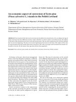
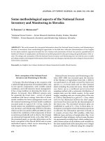
Figure 1 illustrates the simulation of stand development
indicating the optimised and fixed management parameters.
2.2. Economic data
2.2.1. Costs
Logging costs were based on the unit price tariffs of forestry
activities (Cuadro de precios unitarios de la actividad forestal)
published by the Asociación y Colegio de Ingenieros de Montes [2]

and on a study by Montero et al. [19]. The tabulated tariff values were
smoothed to form a model of the total logging cost as a function of
tree size (figure 2):
(7)
where c is logging cost in pesetas

(ptas) m
–3
and dbh is breast height
diameter in cm.
A cost of 1000 ptas m
–3
was added to this cost covering the
removal of cutting residuals [19]. An entry cost of 600 ptas ha
–1
was
also assumed, consisting of the authorisation of logging plus the cost
of marking the trees to log [19]. In addition to these, the costs of a pre-
commercial thinning were assumed to take place in year t after stand
establishment, the tending year depending on site index as follows:
t = 35 – 0.677 ´ SI.(8)
The tending cost was always 100 000 ptas ha
–1
. This cost is based
on data provided by the Forest Technology Centre of Catalonia. The
tending year function was estimated based on a study by Montero
et al. [19] who suggested that the pre-commercial thinning in Scots
pine stands should take place between stand age 15 to 25 years
depending on stand growth. An annual fire protection cost of
1500 ptas ha

–1
[19] was also included in the calculation of soil
expectation value and mean annual income.
2.2.2. Incomes
It was assumed that the road-side timber price is 8000 ptas m
–3
for
the diameter class of 27.5 cm. This price is based on a study by Díaz
Balteiro and Prieto Rodríguez [8] who assumed the price for trees that
were not appropriate for veneer logs. The basic price of 8000 ptas m
–3
of trees larger than 34 cm was multiplied by an index based on the
study of Montero et al. [18]. The index increased with diameter. The
indices have been computed based on the assumption that larger
diameters produce a larger percentage of wood for veneer sheets,
which have a price four times higher than wood without that
characteristic [18]. The price for small diameter classes, mainly
coming from thinnings, was estimated from data collected by the
Forest Technology Centre of Catalonia during the preparation of the
latest forest management plans in 2001. All these tabulated price
values were smoothed to give the road-side price as a function of tree
diameter (figure 2):
(9)
where p is a roadside timber price (ptas m
–3
) and D
p
is dbh (cm) for
trees smaller than 65 cm in diameter, and 65 cm otherwise (i.e. 65 cm
is used if dbh exceeds 65 cm).

2.3. Objective functions
The management schedule of each stand was optimised using soil
expectation value (SEV) as the objective variable, which is defined as
the net present value of all future net incomes [25, 29].
Figure 1. Simulation and optimisation components of a management
schedule with one pre-commercial thinning (dashed line), three
commercial thinnings (thick solid line) and three regenerative cuts
(thin solid line) on site index 24 m (at 100 years) by using the SPINE
system.
c 9.407 0.506 dbh()ln´–[]exp=
Figure 2. Timber prices and harvesting costs data, and the smoothed
price and cost models based on the data points.
p 3867 2268 D
p
´+–=
108 M. Palahí and T. Pukkala
The net present value (NPV) of all the management operations in
a rotation, discounted to the beginning of the rotation, is:
(10)
where N is the net income from a management operation, i is the
discounting rate, t is the year of the operation and R is the rotation
age. The NPV of an infinite series of future harvests is referred to as
the soil expectation value (SEV) and can be computed from:
(11)
The SEV is a justified management objective if a single economic
goal must be selected [17]. The discounting rate used was 2%. Díaz
Balteiro and Prieto Rodríguez [8] proposed this discounting rate
based on the fact that 2% is very close to the rate of return of the
public debt in Spain. Other studies [13] also support the suitability of
this discounting rate value. A sensitivity analysis was conducted

using discounting rates of 1% and 3% to study the effect of this
parameter on the optimal management schedule.
In addition to the SEV, the mean annual net income, i.e. forest rent
(FR), and the mean annual harvested volume (WP) were used as
objective functions to study the sensitivity of the optimal
management to the type of objective variable.
2.4. Decision variables
Optimising the management schedule means finding the optimal
values for a set of decision variables (DV). Because the number of
thinnings is not a continuous variable, schedules with different
number of thinnings are to be treated as separate optimisation
problems. The management regime was specified by the number of
thinnings, and by the DVs, which were chosen as follows:
For each thinning:
– Years since previous thinning, or if it is the first thinning
stand age when the thinning occurs.
– Remaining basal area.
For final cuttings:
– Years since the last thinning to the first regenerative cut.
The number of decision variables (NDV) depends on the number
of thinnings (NTH) as follows:
NDV = 2 ´ NTH + 1. (12)
2.5. Optimisation method
The simulation model described above was linked to the direct
search method of Hooke and Jeeves [12] that was used as the
optimisation algorithm. This algorithm has been commonly used for
optimising the management of both even-aged stands [14, 16, 21, 26,
27, 30] and uneven-aged stands [3, 11, 21]. The direct search method
algorithm operates using two search modes: exploratory search and
pattern search. Given a base point (a vector of DVs), the exploratory

search examines points around the base point in the direction of the
coordinate axes (DVs). The pattern search moves the base point in the
direction defined by the previous base point and the best point of
exploratory search (for more details see [4]).
The combined simulation-optimisation system is capable of
finding the optimal treatment schedule for a given stand, when the
number of thinnings, the economic parameters (timber prices,
harvesting costs, discounting rate, etc.) and the objective variable are
specified. An estimate of the optimal combination of DVs is used as
the initial solution for the optimisation program. The program calls the
simulation sub-system which reads the economic parameters and the
initial stand characteristics and computes the value of the selected
objective variable (objective function). Based on the feed back from
the simulation sub-system, the optimisation sub-system alters the
values of the DVs by using the exploratory and pattern search of
the optimisation algorithm. The simulation sub-system re-calculates
the objective function with the new DVs values. The optimal
management schedule for a given number of thinnings is eventually
found, after repeating this search-process as many times as defined by
a convergence criterion. The optimisation was carried out for 0, 1, 2,
3, 4, and 5 thinnings to find the number of thinnings that maximised
the objective variable.
Because the optimisation algorithm does not necessarily converge
to the global optimum, all optimisations were repeated 51 times, each
run starting from the best of 200 random combinations of DVs,
except the first one, which started from a user-defined starting point.
The random values of DVs were uniformly distributed over a user-
specified range. The following ranges were used:
• year of the first thinning: 5–80;
• intervals of later cuttings: 5–40 years;

• remaining basal area in a thinning: 5–40 m
2
ha
–1
.
These ranges only concerned the random searches in the
beginning of each direct search; the direct search was allowed to go
outside these ranges. The initial step-size in altering the values of
DVs in the direct search was 0.1 times the range. The step size was
gradually reduced during the direct search, and the search stopped
when the step size of all DVs was less than 0.00005 times the initial
range (convergence criterion).
3. RESULTS
3.1. Optimal management schedule
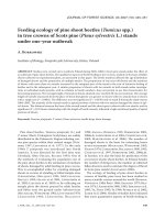
On all site indices (17, 24 and 30 m) five thinnings were
needed to maximise the objective function (figure 3). On site
index 17 the first thinning took place immediately (24 years)
and there was no preparatory cut because the last thinning (at
94 years) left a remaining basal area smaller than 20 m
2
ha
–1
.
NPV
N
t
1 i+()
t

t 1=

R
å
=
SEV
NPV
1
1
1 i+()
R
–
=
.
Figure 3. Development of stand volume in the optimal management
schedule for maximum soil expectation value on site indices 17, 24
and 30 m (at 100 years).
Optimising the management of Scots pine stands in Spain 109
On site index 24, the first thinning took place immediately and
the first regenerative cut (preparatory cut) at a stand age of
70 years, giving an optimal rotation of 90 years with the
20-year shelterwood period. On site index 30 the first thinning
occurred at stand age of 44 years and the preparatory cut at
74 years (rotation age 94 years). The SEV of site indices 17,
24 and 30 was 427812, 1 500 090 and 2 269 111 ptas ha
–1
,
respectively. The mean annual harvest of the optimal regime
was 4.3, 9.1 and 14.7 m
–3
ha
–1

year
–1
, respectively, for site
indices 17, 24 and 30 m.
3.2. Sensitivity analysis
The effect of discounting rate on the optimal schedule is
very clear on all sites (figures 4–6). The higher the discounting
rate, the sooner the final cuttings start (preparatory cut) and
therefore the optimal rotation is shorter. The thinnings become
heavier with increasing discounting rate. This result is logical,
since it is more profitable to decrease the value of the growing
stock, through thinnings and regenerative cuttings, if the
return from alternative investments improves.
The stand volume development for maximising SEV,
volume production, i.e., mean annual harvest (WP), as well as
forest rent (FR) were compared to investigate the sensitivity of
the management schedule to the objective function (figures 7–9).
The results indicate that if WP is maximised the number of
thinnings is reduced to 2 for site index 17 and 1 for site index
24, while no thinnings are needed on site index 30 m. The
mean annual harvest when maximising WP was 5.2, 9.8 and
15.3 m
–3
ha
–1
year
–1
for site indices 17, 24 and 30 m, respec-
tively. The results (figures 7–9) indicate that the better the site
index of the stand the fewer or even no thinnings are needed to

maximise WP.
When FR is maximised the rotations in all site indices are
much longer than maximising SEV or WP. This is due to the
fact that FR, i.e., the mean annual net income, is equivalent to
NPV with 0% discounting rate. Therefore, when maximising
this objective function there are no investment alternatives,
and since the price of wood increases with timber diameter
(until 65 cm of diameter) and harvesting costs per m
3
decrease,
rotations are prolonged as long as diameter growth continues
to be reasonable. For site indices 24 and 30 m the optimal
rotations for maximising FR are 141 years. For site index 17
the optimal rotation for maximising FR is 199 years.
F
igure 4. Optimal management schedule on site index 17 m (at age
100 years) maximising soil expectation value with 1, 2 and 3 percent
discounting rate.
Figure 6. Optimal management schedule on site index 30 m (at age
100 years) maximising soil expectation value with 1, 2 and 3 percent
discounting rate.
Figure 7. Sensitivity of the optimal management schedule on site
index 17 (at age 100 years) to changes in the objective function:
maximum mean annual harvest (WP), maximum soil expectation
value (SEV) and maximum forest rent (FR).
Figure 5. Optimal management schedule on site index 24 m (at age
100 years) maximising soil expectation value with 1, 2 and 3 percent
discounting rate.
110 M. Palahí and T. Pukkala
The sensitivity of SEV, FR and WP to the objective

variable that is maximised is shown in table II. SEV was the
most sensitive to the choice of objective variable, while WP
and FR were less sensitive. The results indicate that, on all site
indices, SEV decreases more when the objective variable is
FR than when it is WP. The mean annual harvest was closer to
the maximum WP when maximising SEV than when FR was
maximised. Furthermore, the relative sensitivity of SEV, FR
and WP to a change in the objective variable is greater on site
index 17 than on the other two sites.
The sensitivity of the objective function value (SEV) to
changes in the values of the DVs was tested on site index 24
by increasing or decreasing the value of one DV at a time by
10%, 20% and 30% and re-simulating the management
schedule. The SEV was not sensitive to small changes in the
DVs (table III). The SEV was the most sensitive to changes in
the DVs of the first thinning. The later the change in the DVs
took place, the smaller was the change in SEV. From the two
DVs that characterised each thinning (years since previous
thinning and remaining basal area after thinning) the latter one
appeared to have more influence on SEV.
The optimisations of thinnings and rotation length for each
number of thinnings constitute different problems with corre-
sponding numbers of variables. The number of thinnings is
therefore a parameter given to the simulation-optimisation
system at the outset. The maximum SEV for 0, 1, 2, 3, 4 and 5
thinnings on site indices 17, 24 and 30 are shown in figure 10.
Although soil expectation value increased with the number of
thinnings until the optimum was reached, most of the gain was
achieved with just one thinning. Three and four thinnings were
practically equally good as the optimal number (i.e., 5 thinnings).

Timber prices and variable harvesting costs were another
set of uncertain parameters. We analysed the sensitivity of
stand management to prices and costs changes by increasing
or decreasing the values of each of these parameters at a time
by 15% and 30% and re-computing the optimal solution. The
results indicate that the optimal management schedule with the
SEV as the objective was not very sensitive to the level of
timber prices (figure 11) and variable harvesting costs
(figure 12). The rotation length was prolonged 10 years when
the prices decreased 30% and 5 years when harvesting costs
were increased 30%. The optimal rotation was 10 years
Table II. Soil expectation value (SEV, 1000 ptas ha
–1
), forest rent (FR, 1000 ptas ha
–1
year
–1
), and mean annual harvest (WP, m
3
ha
–1
year
–1
)
in the optimal schedule when maximising the variable in the first column.
Objective Site 17 Site 24 Site 30
variable SEV FR WP SEV FR WP SEV FR WP
SEV 428 24.5 4.3 1500 58.3 9.1 2269 87.9 14.7
FR 245 32.0 3.8 1134 68.1 8.1 1811 101.1 12.4
WP 328 19.0 5.2 1399 53.8 9.8 2089 75.9 15.3

Figure 8. Sensitivity of the optimal management schedule on site
index 24 (at 100 years) to changes in the objective function:
maximum mean annual harvest (WP), maximum soil expectation
value (SEV) and maximum forest rent (FR).
Figure 9. Sensitivity of the optimal management schedule on site
index 30 (at 100 years) to changes in the objective function:
maximum mean annual harvest (WP), maximum soil expectation
value (SEV) and maximum forest rent (FR).
Figure 10. Sensitivity of the maximal SEV to the number o
f
thinnings on site indices 17, 24 and 30 m (at age 100 years).
Optimising the management of Scots pine stands in Spain 111
shorter when harvesting costs decreased by 30%. In general,
thinnings began later when timber prices decreased or
harvesting costs increased.
The fixed entry cost of thinning was based on the
administrative and marking costs presented by Montero et al.
[19]. These costs are rather low. The sensitivity of optimal
management to increased entry costs was analysed in the plot
with site index 24 m (figure 13). Figure 13 shows that
increasing entry costs reduce the number of thinnings and the
thinnings became heavier. The entry costs do not affect much
the length of the optimal rotation.
4. DISCUSSION
The results of this study are based on the models of Palahí
et al. [22, 23]. The optimisations for site index 17, when
maximising FR, are not as reliable as the other results because
a long extrapolation beyond the maximum stand age of the
modelling data [23] was required (rotation of 199 years). The
results for the plot with site index 30 m may also be less

reliable than the results for the other sites due to an
extrapolation beyond the maximum site index of the
modelling data. However, although the maximal stand
Table III. Sensitivity of soil expectation value (1000 ptas ha
–1
) on site index 24 to changes in decision variables (DVs). The optimal values of
DVs for each thinning and the first final cut, i.e., number of years since previous thinning (Y), remaining basal area after thinning (Gr) and
years since last thinning to the first final cut (Yc), were independently increased and decreased by 10, 20 and 30 percent. After these changes
the SEV was calculated again.
–30% –20% –10% Optimum +10% +20% +30%
First thinning
Y -* - 1499.9 1500.0 1486.7 1477.4 1463.4
Gr 1460.2 1482.9 1496.0 1500.0 1483.2 1474.4 -
Second thinning
Y 1496.9 1497.0 1498.1 1500.0 1497.1 1494.7 1492.6
Gr 1481.6 1492.4 1498.1 1500.0 1498.0 1492.9 1485.9
Third thinning
Y 1498.2 1498.7 1499.3 1500.0 1497.9 1495.9 1493.9
Gr 1491.7 1496.6 1499.2 1500.0 1498.8 1496.2 1492.7
Fourth thinning
Y 1498.9 1499.1 1499.5 1500.0 1499.3 1498.7 1498.1
Gr 1493.1 1497.0 1499.3 1500.0 1499.3 1497.5 1496.3
Fifth Thinning
Y 1498.9 1499.2 1499.6 1500.0 1499.4 1498.9 1498.3
Gr 1491.1 1496.0 1498.9 1500.0 1499.2 1497.0 1493.2
Preparatory cut
Yc 1499.5 1499.6 1499.8 1500.0 1498.7 1497.4 1496.1
*
Dashes correspond to situations that could not be simulated because the value of the DV was out of the range of the possible development of the stand.
Figure 12. Sensitivity of the optimal management schedule to

increasing and decreasing harvesting costs.
Figure 11. Sensitivity of the optimal management schedule to
increasing and decreasing timber prices.
112 M. Palahí and T. Pukkala
volumes that the simulator produced for site index 30 m are
very high (figure 9) they are in accordance with the yield
tables presented by Rojo and Montero (1996) and used in
Montero et al. (1996) for site index 30 m. The set of models
used in the simulation program were based on permanent
sample plots that ranged from 33 to 148 years in age and from
14 to 26 m in site index [22, 23]. In stands younger than
148 years the models have been found to follow accurately the
measured stand development of permanent sample plots [23].
The reliability of the optimisation algorithm was tested by
repeating the optimisation for site index 24 with 3 thinnings
for 100 times, each time starting from a different random
solution, and analysing the variation among solutions. The
standard deviation of soil expectation value was 7223 ptas ha
–1
,
which is 0.49% of the mean. The standard error of mean was
only 0.049%. The standard error of rotation length was 0.055
years, which is 0.085% of the mean. In fact the optimal
rotation was practically the same (differences were smaller
than 0.05 years) in 98 out of 100 solutions, and 4 years shorter
in 2 solutions. The timing of thinnings varied more but the
changes were always mutual so that if the interval between
two thinnings decreased by, for example, 5 years compared to
the previous solution, the next interval increased by 5 years.
The length of these swaps was typically about 5 years. The

remaining basal area was always practically the same for a
given thinning year. The results indicate that the optimisation
method was able to find the maximal SEV and optimal
rotation with high precision but the optimal timing of
thinnings is less precise (it is found with 5-year accuracy). The
reason for this uncertainty is that several combinations of
cutting intervals are almost equally good, i.e. they produce
almost exactly the same SEV
.
Although the optimal management of Scots pine stands was
not very sensitive to changes in the level of prices, the use of
the non-smoothed prices instead of the price model (see figure 2)
produced a completely different optimal management schedule.
Figure 14 shows that using the non-smoothed prices, a very
heavy thinning takes place immediately when the minimum
diameter reaches 20 cm. When non-smoothed prices are used,
logging of 20 cm trees produces a distinctly greater net income
than logging of trees slightly smaller than 20 cm (see figure 2).
In addition, increasing tree diameters up to 40 cm improves
the unit price only very little. This comparison shows that it is
advisable to carefully check that the information concerning
timber prices and harvesting costs are valid for each particular
situation in which optimisations are done. The results concerning
the sensitivity of the optimal management schedule to changes
in the fixed entry costs is in accordance with the study by
Filius and Dull [9], which shows that the number of thinnings
decreases with increasing fixed entry costs, but rotation length
is not much affected.
We are aware of the problems related to the simulation of
the same shelterwood cuttings in all optimisations. Previous

studies in Spain [28] indicate that it is difficult to specify a
single treatment schedule of the uniform shelterwood method
for all Scots pine stands in Spain because the system depends
on the characteristics of each stand. In this study, the simulated
reproductive method is based on a traditionally accepted
20-year period for regenerating Scots pine stands in Spain [19]
and on previous studies in Spain [15] that concluded that an
average basal area of 12 to 15 m
2
ha
–1
is adequate to obtain
good regeneration in stands of Scots pine. Although
technically possible, it was not reasonable to optimise the
intervals and post-cutting basal area of the regenerative cuts
because the exact relationship between cutting parameters and
regeneration result was unknown. Further studies on the
density and population structure of natural regeneration such
as the one presented by González-Martínez and Bravo [10] are
needed to treat the regenerative cuttings as decision variables
in the optimisation process.
The analysis conducted in this study indicates that the
optimal management schedule of Scots pine stands on site
indices 17, 24 and 30 m are sensitive to the management goal.
Maximising WP produces management schedules with fewer
thinnings than maximising SEV or FR. The results also show
that the better the site index of the stand the fewer thinnings
are needed to maximise WP. On site indices 17, 24 and 30 m,
2, 1 and 0 thinnings were needed to maximise WP. Maximising
FR calls for much longer rotations than maximising SEV or WP.

The results shown in figure 3, which suggests longer rotations
Figure 14. Stand basal area in the optimal management schedule fo
r
site index 24 with 2% discounting rate and 3 thinnings when using
smoothed and non-smoothed timber prices, and the mean diamete
r
development when the non-smoothed price function is used in
optimisation.
Figure 13. Sensitivity of the optimal management schedule to
increasing fixed entry costs on site index 24 m with 2% discounting
rate.
Optimising the management of Scots pine stands in Spain 113
for site index 30 m than for site index 24 m, can be explained
by the different initial stand characteristics (diameter
distributions) of the two plots.
The results of our optimisations agree fairly well with the
previous recommendations by Montero et al. [18, 19], which
suggest maximising forest rent and having rotations of 100 to
140 years depending on the site index and the thinning regime.
However, in this study SEV was considered to be the most
reasonable economic management goal [17]. With the SEV
goal, the optimal management schedule was sensitive to the
discounting rate, the rotation being shorter and the thinnings
earlier and heavier for higher discounting rates. The
insensitivity of SEV to changes in any single decision variable
indicates that the objective function is a flat function of DVs
near the optimum.
The applicability of the system presented depends on the
production objectives of the forest. Clutter et al. [6] divided all
timber management planning situations into two distinct

categories: (1) those situations in which planning can be done
independently for each stand; and (2) those situations in which
the planning must be co-ordinated for all stands in the forest
being considered. The first situation, referred to as stand-level
management planning, assumes that each stand is treated in
the way that will best meet the goal of the forest owner. In this
situation, the stand management support system described in
this study can be used directly. Also, the system could be used
to produce management instructions for different sites and
stand densities. In addition, stand-level optimisations serve
comparative analyses on the effects of economic or biological
factors on stand management [31].
However, the majority of forests cannot be managed
relying only on the stand-level approach because this often
produces large fluctuations in annual harvests and revenues.
Thus, in situations where stable patterns of income are
important, the optimum treatment of a stand will depend on
the rest of the forest property, calling for forest-level
management planning, corresponding to the second category
of Clutter et al. [6]. In this situation, the simulation sub-system
may be used to produce relevant information about alternative
treatment schedules of stands. This information is then
collected into a forest level optimisation model, which is
solved using linear programming or other procedures. Stand-
level optimisation may be used to guide the simulation of
stand management alternatives in forest level planning.
Acknowledgements: Financial support for this project was given
by the Forest Technology Centre of Catalonia (Solsona, Spain). We
thank Dr. Gregorio Montero (Spain) for his helpful suggestions. We
thank Mr. Tim Green for the linguistic revision of the manuscript and

Mr. Jo Van Brusselen for the French translation of the abstract.
REFERENCES
[1] Arthaud G.J., Pelkki M.H., A comparison of dynamic programming
and A* in optimal forest stand management, For. Sci. 42 (1996)
498–503.
[2] Asociación y colegio de Ingenieros de Montes, Cuadro de precios
unitarios de la actividad forestal, Madrid, 2000, 260 p.
[3] Bare B.B., Opalach D., Optimizing species composition in uneven-
aged forest stands, For. Sci. 33 (1987) 958–970.
[4] Bazaraa M.S., Shetty C.M., Nonlinear programming: Theory and
algorithms, Wiley, New York, 1979, 560 p.
[5] Brodie J.D., Adams D.M., Kao C., Analysis of economic impacts
on thinning and rotation for Douglas-fir, using dynamic
programming, For. Sci. 24 (1978) 512–522.
[6] Clutter J.L., Forston J.C., Piennar L.V., Brister G.H., Bailey R.L.,
Timber management – a quantitative approach, Wiley, New York,
1983.
[7] Daniel T., Helms J., Baker F., Principles of silviculture, 2nd edn.,
McGraw-Hill, USA, 1979, pp. 446–447.
[8] Díaz Balteiro L., Prieto Rodríguez A., Modelos de planificación
forestal basados en la programación lineal. Aplicación al monte
“Pinar de Navafria” (Segovia), Invest. Agr.: Recur. For. 8 (1999)
63–92.
[9] Fillius A.M., Dull M.T., Dependence of rotation and thinning
regime on economic factors and silvicultural constraints: results of
an application of dynamic programming, For. Ecol. Manage. 48
(1992) 345–356.
[10] González-Martínez S.C., Bravo F., Density and population
structure of the natural regeneration of Scots pine (Pinus sylvetrsis
L.) in the High Ebro Basin (Northern Spain), Ann. For. Sci. 58

(2001) 277–288.
[11] Haight R.G., Monserud R.A., Optimizing any-aged management
of mixed-species stands: II. Effects of decision criteria, For. Sci. 36
(1990) 125–144.
[12] Hooke R., Jeeves T.A., “Direct search” solution of numerical and
statistical problems, J. Assoc. Comput. Mach. 8 (1961) 212–229.
[13] Kula E., The economics of forestry: Modern theory and practice,
Croom and Helm, London, 1988, 185 p.
[14] Mabvurira D., Pukkala T., Optimising the management of
Eucalyptus grandis (Hill) Maiden plantations in Zimbabwe, For.
Ecol. Manage. 166 (2002) 149–157.
[15] Martínez de Pisón M., Defensa del método denominado “ordenar
transformando”. Escuela de Ingenieros de Montes, Madrid, 1948,
108 p.
[16] Miina J., Optimizing thinning and rotation in a stand of Pinus
sylvestris on a drained peatland site, Scan. J. For. Res. 11 (1996)
182–192.
[17] Miina J., Preparation of stand management models using
simulation and optimisation, in: Pukkala T., Eerikäinen K. (Eds.),
Tree seedling production and management of plantation forests,
University of Joensuu, faculty of Forestry, research notes 68, 1998,
pp. 153–163.
[18] Montero G., Rojo A., Alia R., Determinación del turno de Pinus
sylvestris en el Sitema Central, Montes, 29 (1992) 42–48.
[19] Montero G., Rojo A., Del Rio M., Aspectos selvícolas y
económicos de los pinares de Pinus sylvestris L. en el Sistema
Central, proceedings of the open seminar: “Explotación y
conservación del monte mediterráneo: una apuesta para el futuro”,
Unversidad de Málaga, Ronda, Málaga, 1996.
[20] Montero G., Cañellas I., Ortega C., Del Rio M., Results from a

thinning experiment in a Scots pine (Pinus sylvestris L.) natural
regeneration stand in the Sistema Ibérico Mountain Range (Spain),
For. Ecol. Manage. 145 (2001) 151–161.
[21] Muchiri M., Pukkala T., Miina J., Optimising the management of
maize Grevillea robusta fields in Kenya, Agroforestry systems
56 (2002) 13–25.
[22] Palahí M., Tomé M., Pukkala T., Trasobares A., Montero G., Site
index model for Scots pine (Pinus sylvestris L.) in north-east Spain,
For. Ecol. Manage. (submitted).
[23] Palahí M., Pukkala T., Miina J.,

Montero G., Individual-tree growth
and mortality models for Scots pine (Pinus sylvestris L.) in north-
east Spain, Ann. For. Sci. 60 (2002) 1–10.
[24] Pita Carpenter A., Tablas de cubicación por diámetros normales y
alturas totales, Instituto Forestal de Investigaciones y Experiencias,
Ministerio de Agricultura, Madrid, 1967.
[25] Price C., The theory and application of forest economics, Basil
Blackwell, Oxford, 1989, 402 p.
114 M. Palahí and T. Pukkala
[26] Rautiainen O., Pukkala T., Miina J., Optimising the mangement of
even-aged Shorea robusta stands in southern Nepal using individual
tree growth models, For. Ecol. Manage. 126 (1999) 417–429.
[27] Roise J.P., An approach for optimizing residual diameter class
distributions when thinning even-aged stands, For. Sci. 32 (1986)
871–881.
[28] Rojo A., Montero G., El pino silvestre en la Sierra de Guadarrama,
Centro de publicaciones del Ministerio de Agricultura, Pesca y
Alimentación, 1996, 293 p.
[29] Rose D.W., Brand G.J., Guide to forest investment analysis. USDA

Forest Service Research Paper NC-284, North Central Forest
Experiment Station, St. Paul, MN, 23 p.
[30] Valsta L., A comparison of numerical methods for optimizing even
aged stand management, Can. J. For. Res. 20 (1990) 961–969.
[31] Valsta L., An optimization model for Norway spruce management
based on individual-tree growth models, Acta Forestalia Fennica
232 (1992) 20 p.
To access this journal online:
www.edpsciences.org