Báo cáo lâm nghiệp: "Sustainable cutting cycle and yields in a lowland mixed dipterocarp forest of Borneo" docx
Bạn đang xem bản rút gọn của tài liệu. Xem và tải ngay bản đầy đủ của tài liệu tại đây (427.82 KB, 12 trang )
803
Ann. For. Sci. 60 (2003) 803–814
© INRA, EDP Sciences, 2004
DOI: 10.1051/forest:2003075
Original article
Sustainable cutting cycle and yields in a lowland mixed dipterocarp
forest of Borneo
Plinio SIST
a
, Nicolas PICARD
b
, Sylvie GOURLET-FLEURY
c
*
a
Convênio Cirad-Forêt-EMBRAPA Amazonia Oriental, Travessa Eneas Pinheiro, Belem PA 66095-100, Brazil
b
Cirad-Forêt, BP 1813, Bamako, Mali
c
Cirad-Forêt, TA/10D, 34398 Montpellier Cedex 5, France
(Received 19 February 2002; accepted 19 December 2002)
Abstract – Based on a 6 year monitoring of the dynamics of a mixed dipterocarp forest in East Borneo (1990-1996), we built a matrix model
to predict the sustainable cutting cycle in relation with the extraction and damage rates. Plots were ordered according to three main groups of
damage and logging intensity. The first group G1 gathered slightly damaged plots with a remaining basal area ≥ 80% of the original (mean
logging intensity = 6 trees ha
–1
). Plots belonging to G2, had a remaining basal area varying between 70 and 79% of the original one (mean logging
intensity = 8 trees ha
–1
). Finally, G3 gathers highly damaged plots with a remaining basal area < 70% of the original one and a high logging
intensity (mean = 14 trees ha
–1
). The mean sustainable cutting cycles predicted in the three groups were significantly different and equal 27, 41 and
89 years in G1, G2 and G3 respectively. However, the respective mean annual extracted volumes were similar: 1.6, 1.8 and 1.4 m
3
ha
–1
year
–1
,
respectively in G1, G2 and G3. The model suggests that a 40 year cycle, extracting 8 trees ha
–1
(60 m
3
ha
–1
) and an annual volume of 1.5 m
3
ha
–1
year
–1
is the best option to preserve ecological integrity of the forest, to ensure yield sustainability and, according to existing cost analysis,
economic profitability. This result is also consistent with other studies which already demonstrated that logging damage reduction using RIL
techniques could be only significant with a moderate felling intensity not exceeding 8 trees ha
–1
. This felling intensity threshold can be easily
achieved by applying simple harvesting rules.
dipterocarp forest / sustainable logging intensity / East Kalimantan / TPTI, modeling / reduced-impact logging (RIL) / matrix models
Résumé – Durée de rotation et production durable d’une forêt mixte à Diptérocarpacées de Bornéo. En nous basant sur un suivi de 6 ans
de la dynamique d’une forêt mixte à Diptérocarpacées, de Kalimantan Est (1990–1996), nous avons construit un modèle matriciel pour établir
la période de rotation durable en fonction de l’intensité de l’exploitation et des dégâts engendrés. Les parcelles ont été classées dans trois
groupes de dégâts et d’intensités d’exploitation. Le groupe G1 rassemble des parcelles ayant subi des dégâts peu importants et ayant conservé
une surface terrière ≥ 80 % de l’originale (intensité moyenne d’exploitation = 6 arbres ha
–1
). Les parcelles de G2 ont une surface terrière résiduelle
variant entre 70 et 79 % de l’originale (intensité moyenne = 8 arbres ha
–1
). Enfin G3 regroupe des parcelles fortement perturbées avec une
surface terrière inférieure à 70 % de l’originale et ayant subi une intensité d’exploitation beaucoup plus élevée (14 arbres ha
–1
). Les durées
moyennes de rotation dans les trois groupes sont significativement différentes et s’élèvent à 27, 41 et 89 ans respectivement dans G1, G2 et G 3.
Cependant, les volumes annuels prélevés sont statistiquement similaires : 1.6, 1.8 et 1.4 m
3
ha
–1
an
–1
, respectivement dans G1, G2 et G3. Le modèle
suggère qu’un cycle de 40 ans, avec une extraction moyenne de 8 arbres ha
–1
(60 m
3
ha
–1
) et un volume annuel prélevé de 1.5 m
3
ha
–1
an
–1
constitue la meilleure option permettant d’assurer l’intégrité écologique de la forêt, ainsi qu’une production constante et, selon les études de
coûts existantes, économiquement rentable sur le long terme. Ce résultat conforte par ailleurs les études précédentes ayant démontré que les
dégâts d’exploitation ne pouvaient être réduits de façon significative grâce à l’EFI (exploitation à faible impact) qu’à condition de limiter
l’intensité d’extraction à 8 arbres ha
–1
. Des règles simples permettent de respecter cette intensité.
forêt mixte à Diptérocarpacées / intensité d’exploitation durable / Kalimantan Est / TPTI / modélisation / exploitation à faible impact
(EFI) / modèles matriciels
1. INTRODUCTION
In Borneo where primary lowland forests exhibit a high
density of harvestable trees (23 ha
–1
> 50 cm dbh and 16 ha
–1
> 60 cm, diameter cutting limit depending on the type of for-
est), logging operations commonly damage more than 50% of
the original stand [4, 22, 30, 32, 37]. These heavy cuts result
in a seriously depleted residual stand, which is unlikely to
reach an acceptable harvesting volume within a cutting cycle
of 35 years as set up by the Indonesian regulations [16, 42].
The low economic value of those intensively logged forests
makes them prone to be converted into agriculture lands.
Moreover, large canopy openings and heavy vine invasion
occurring in over-logged forests increase vulnerability to fire
* Corresponding author:
804 P. Sist et al.
as was dramatically demonstrated in Indonesia during the
recent past successive El Niño drought events [25]. Detailed
observations over several decades of forest dynamics proc-
esses after logging, based on permanent sample plots where
ecological conditions were recorded before and after harvest-
ing, are still lacking in South East Asia and, generally speak-
ing in tropical forests [18, 34, 44]. This situation led to develop
a wide range of forest dynamics models to predict forest yield
and dynamics after disturbance [39, 52, 53]. These models
were individual-based models with space-independent [9, 20,
23, 34, 39, 51, 54] or space-dependent [18, 28, 35, 36] interac-
tions, as well as distribution-based (or matrix) models [5–8,
15, 16, 21]. During this last decade, these models originally
research oriented, have been developed to a more practical
approach integrating silvicultural and logging practices, to
become effective management tools [1, 26]. Contrary to indi-
vidual-based models, matrix models provide limited insights
into the possible processes that drive the forest dynamics.
However, they offer the advantage to use mostly discrete
diameter distributions which are easy to assess in the field on
relatively large areas. Moreover, matrix models can also pre-
dict in a robust way and as reliably as other approaches, stand
structure (density, basal area and diameter distribution) and
are mathematically more tractable than individual-based models.
For these reasons these models are generally considered as
efficient tools for the management of tropical forests, which
generally include large production areas but where inventories
are very limited. This paper aims at simulating the impact of
logging intensity and associated damage to assess the most
suitable felling cycle able to ensure a long-term sustainable
timber production. This will help to evaluate the Indonesian
Selective System, better known as TPTI, recommending a 35-
year felling cycle period. For this, we built a matrix model
based on a 6 year monitoring of a mixed dipterocarp forest in
East Borneo (1990–1996).
2. STUDY SITE AND METHODS
2.1. The STREK experimental design
2.1.1. Study site
The study area is located in the Indonesian province of East Kali-
mantan (Borneo Island), in the district of Berau, near Tanjung Redeb
(2° N, 117° 15E), within a 500 000 ha forest concession [3]. The cli-
mate is equatorial with a mean annual rainfall of about 2000 mm.
August is the driest month with a mean of 90 mm rainfall and January
the wettest with 242 mm (data for Tanjung Redeb over the period
1984–1993). The bedrock is primarily alluvial deposits (mudstone,
siltstone, sandstone and gravel) dating from the Miocene and
Pliocene. Soils are mainly Ultisols (87.3%), with some Entisols
(10.7%) and Inceptisols (2%). The topography is gently undulating to
hilly in the north, changing to steep slopes with elevations reaching
500 m above sea level in the south.
2.1.2. Experimental design and treatments
A 5% inventory of the 1000 ha zone scheduled for logging pro-
vided the database for sample plot selection [3]. Twelve 4 ha plots
(200 m × 200 m) each divided into four 1 ha squares or subplots, were
set up from 1990 to 1991. All trees with dbh ≥ 10 cm were measured
(girth at 1.30 m or 20 cm above buttresses), numbered and mapped on
a scale of 1/200. In control plots, all trees were identified to species
from 1990 to 1993 whereas in the other 9 logged plots, tree identifi-
cation was performed to species for dipterocarps but to genus or fam-
ily level only for the other taxa [43].
Logging operations were carried out from November 1991 to May
1992, in the 1000 ha annual coupe area including the permanent sam-
ple plots. Four different treatments were defined, each treatment
being replicated three times. Treatments included two Reduced-
Impact Logging techniques (2 × 3 plots), a conventional logging
method (3 plots) and, finally, an unlogged control treatment including
3 plots [4]. Owing to the Indonesian silvicultural system, harvesting
was limited to trees larger than 60 cm of the following dipterocarp
species Anisoptera spp., Dipterocarpus spp., Dryobalanops beccarii,
Hopea spp., Parashorea spp. and Shorea spp. Two years after logging
(1994), in the logged plots, all trees with bad damage such as those
leaning or with a broken bole were cut (trees with dbh ≤ 20 cm) or
poisoned (dbh ≥ 20 cm). On average, for the 36 subplots concerned,
19 trees ha
–1
(SD = 9.8) or 0.70 m
2
ha
–1
(SD = 0.42) were removed
during this treatment. This was not taken into account for the calcu-
lation of “natural mortality” after logging.
2.1.3. Plot monitoring
Four successive measurements were carried out between 1990 and
1996. The first one occurred before logging, during plot set up in
1990–1991. The second was performed 3 months after logging
between May and August 1992, the third and fourth ones every two
years in 1994 and 1996 respectively and during the same year period
(May–August). At each census, we recorded girth of all living indi-
viduals 10 cm dbh to the nearest mm with a fibreglass girth tape,
new trees with dbh 10 cm, dead trees and causes of mortality. During
the entire census period, 1990–1996, a total of 28657 trees were
measured, monitored and recorded in the database.
2.1.4. Subplots groupings
There was a positive and significant correlation between the pro-
portion of stems damaged and basal area removed (R
2
= 0.62, P =
0.01, n = 36, [4]). This result suggested that felling intensity was an
important feature in the damage caused by logging regardless of the
technique (reduced-impact logging or conventional, [42]). Two years
after logging, there was a negative correlation between post-logging
mortality (% year
–1
) and the proportion of remaining basal area after
logging (R
2
= 0.43, [29]). To assess the effect of logging damage
intensity on forest dynamic processes, regardless of the logging tech-
niques, we ordered the 48 subplots according to the proportion of
remaining basal area (basal area after logging/original basal area
before logging in %). The average remaining basal area of all the
plots being 74% of the original one, we defined the three groups to
obtain a fair distribution of the 48 subplots, as follows:
Group 0 (G0): Control plot, unlogged, no damage, 100% of the initial
basal area (n = 12 subplots);
Group 1(G1): Low damage rates with a remaining basal area 80%
of the original one (n = 11 subplots);
Group 2 (G2): Moderate damage rates with a remaining basal area =
70–79% of the original one (n = 14 subplots);
Group 3 (G3): High Damage rates with a remaining basal area < 70%
(n = 11 subplots) of the original one.
Before logging, mean (± SD, n = 48 subplots) tree density (dbh
10 cm), basal area and standing volume in the 12 plots were respectively
530 ± 71.6 stems ha
–1
, 31.5 ± 4.2 m
2
ha
–1
and 402.0 ± 61.0 m
3
ha
–1
(Tab. I). In the plots, logging intensity ranged from 1 to 17 ha
–1
(9 m
3
ha
–1
to 247 m
3
ha
–1
) and averaged 9 trees ha
–1
(86.9 m
3
ha
–1
, [4]). Mean
density of harvested trees varied from 6 trees ha
–1
in G1 to 14 trees
ha
–1
in G3 and were significantly different in the three groups
≥
≥
≥
≥
Sustainable felling cycles in Borneo forests 805
(ANOVA, F = 22.71 P < 0.001, Tab. I). After logging, mean basal
areas remaining in the three groups varied from 17.3 m
2
ha
–1
in G3
to 28.3 m
2
ha
–1
in G1 (Tab. I).
2.2. Theoretical growth model: General concept
We used a Usher matrix model [48, 49] with the modifications by
Buongiorno and coworkers [10–12, 15], that is based on species
groups and density-dependent coefficients. A living tree of species
group s, in the diameter class i at time t will at time t + ∆t, either:
– die with the probability m
si
(t),
– stay alive and move up from class i to class i+1 with the prob-
ability a
si
(t),
– stay alive in the same diameter class i with the probability
1 – m
si
(t) – a
si
(t).
Let y
si
(t) be the number of trees of species group s in diameter
class i at time t, F
s i
→
j
(t) the number of trees of species group s mov-
ing from diameter class i to j (= i + 1) between t and t + ∆t, and
F
si
→
dead
(t) the number of trees of species s in diameter class i that
die between t and t + ∆t . Following the Markov chain interpretation
model, (F
s i
→
i+1
, F
s i
→
i
, F
s i
→
dead
) is a random vector that follows a
multinomial law with parameters (y
si
, a
si
, 1 − m
si
− a
si
, m
si
). The Usher
model may also be formulated in a deterministic way by writing:
F
si
→
i+1
= a
si
y
si
, F
s i
→
i
= (1 − m
si
− a
si
)y
si
and F
s i
→
dead
= m
si
y
si
. In
both stochastic and deterministic way, the stand dynamics between
t and t +∆t is expressed by the following equation:
y
s i
(t + ∆t) = F
s i – 1
→
i
(t) + F
s i
→
i
(t). (1)
Taking into account the number of trees newly recruited in the first
diameter class, equation (1), in the deterministic case, can be written
in its matrix form as:
Y
s
(t+∆t) = A
s
(t) Y
s
(t) + r
s
(t), (2)
where Y
s
is the vector of the number of trees in each diameter class
for species group s, A
s
, the transition matrix containing the m
si
and
a
si
probabilities, r
s
the vector for recruitment.
The expression for the A
s
matrix is:
1 – a
s1
– m
s1
0
a
s1
.
.
.
.
.
.
1 – a
si
– m
si
a
si
.
.
.
0
.
.
.
1 – m
sk
r
s
and for the r
s
vector: 0
. .
.
.
0
From equation (2), the dynamics of the whole stand can be written as
follows:
Y(t+∆t) = A(t)
Y(t) + R(t) (3)
where Y is the vector of the whole tree population, R is the vector
[r
1
r
S
] and A is the transition matrix containing the transition matri-
ces A
s
:
where S is the number of species.
Taking into account the number of harvested trees and those
destroyed during logging operations, included in the vector H(t),
equation (3) becomes:
Y(t+∆t)
= A(t)
[ Y(t)
– H(t)] + R(t). (4)
Thus Y(t) – H(t) includes the undamaged trees and the damaged trees
(i.e. the trees wounded by logging operations but still standing).
Tabl e I. Mean stand characteristics of the four groups of plots (± SD) before (year 1990) and after (year 1992) logging.
Group 0 Group 1 Group 2 Group 3
Number of 1 ha subplots 11 11 14 11
Pre-harvest (1990)
Mean density (1990) 527.9 ± 56.9 557.7 ± 71.9 540.2 ± 80.3 481.9 ± 55.6
Mean basal area (m
2
ha
–1
) 30.7 ± 3.1 32.8 ± 4.9 31.8 ± 5.5 29.5 ± 1.7
Mean density of dipterocarps (trees ha
–1
) 109.3 ± 23.0 139.4 ± 43.0 113.1 ± 35.1 104.5 ± 28.1
Mean basal area of dipterocarps (m
2
ha
–1
) 14.5 ± 2.9 15.5 ± 3.6 14.8 ± 3.6 15.7 ± 3.1
Post harvest (1992)
Mean felling intensity (harvested trees ha
–1
) – 5.8 ± 2.3 8.2 ± 3.3 13.9 ± 3.0
Mean % of injured trees – 15.3 ± 5.6 21.5 ± 6.0 25.4 ± 5.5
Mean % of trees killed – 14.8 ± 4. 6 22.0 ± 4.9 33 ± 6.7
Mean % of basal area remaining – 86.2 ± 4.6 75.4 ± 19.7 58.6 ± 7.7
Mean density after logging (trees ha
–1
) 524.1 ± 54.7 486.4 ± 80.3 429.4 ± 65.4 331.0 + 64.2
Mean basal area after logging (m
2
ha
–1
) 30.7 ± 3.2 28.3 ± 4.9 23.9 ± 3.6 17.3 ± 2.7
Mean density of dipterocarps (trees ha
–1
) 108.1 ± 23.0 117.9 ± 34.9 85.8 ± 26.1 63.6 ± 20.8
Mean basal area of dipterocarps (m
2
ha
–1
) 14.5 ± 3.1 12.4 ± 3.3 9.3 ± 2.2 6.4 + 2.3
A
1
0 . . . 0
0
.
.
.
.
.
.
.
.
.
.
.
.
.
.
.
.
0
.
.
0 . . . 0 A
s
806 P. Sist et al.
2.3. Construction of the model using STREK data
2.3.1. Species grouping
Three main groups of species, called S
1
, S
2
, S
3
were distin-
guished.
S
1
gathers all pioneer species that are defined here as those requir-
ing full penetration of light to the forest floor for the germination of
seeds and establishment of seedlings [45]. The most common species
in the study area were Anthocephalus chinensis (Lam.) Rich., Dua-
banga moluccana Bl., Macaranga gigantea (Reichb. f. & Zoll.)
Muell. Arg., M. hypoleuca (Reichb. f. & Zoll.) Muell. Arg., M. tri-
loba Muell. Arg., Octomeles sumatrana Miq. S
2
includes all diptero-
carps, except the genus Vatica which, in contrast with all the other
dipterocarps, has no commercial value. S
3
represents all the other species
including those of the genus Vatica.
This species grouping mainly aimed to follow separately the
dynamics of the commercial species (i.e. dipterocarps) and that of
pioneers after logging but not to reflect the changes in species com-
position or diversity after logging. Group S
1
gathers species with a
very similar ecological behaviour, as they all require full light to ger-
minate and to develop. This group is homogeneous enough to be con-
sidered as a guild of species. Although dipterocarps include a wide
range of species, they share common ecological behaviour that allows
for their categorisation in the same guild of regeneration. Seeds
require partial canopy shade protection for germination and early sur-
vival but they also require an increase of light, as this occurs after log-
ging, for further establishment and growth [2, 17, 27, 31, 47].
Response of dipterocarps in the later development stage is also strong
as growth of trees (dbh ≥ 10 cm) is clearly stimulated by canopy
opening resulting from logging [29, 41]. Compared with the other
two groups, S
3
is undoubtedly the most heterogeneous, including dif-
ferent species with different ecological behaviours. This group can-
not be therefore regarded as a guild or functional group as commonly
defined in ecological studies.
2.3.2. Specific equations
The basic unit of the model is each subplot of 1 ha ordered into the
four groups of damage. Time step ∆t is 2 years, the time interval
between the two successive post-logging measurements. The diame-
ter classes width was adjusted according to the group of species in
order to obtain fluxes F
s i
→
i+1
= a
si
y
si
large enough. For the diptero-
carps (S
2
), we defined 9 classes ranging from 10 to 90 cm dbh with a
constant 10 cm width, the last one gathering all trees with
dbh ≥ 90 cm. For the pioneer species group (S
1
), only 3 dbh classes
were defined (10–20, 20–30 and ≥ 30 cm) as only very few trees reach
a dbh ≥ 30 cm. For S
3
, the sample of trees was large enough to define
10 dbh classes with a constant 5 cm width for the dbh between 10 and
55 cm, the last class including all trees with dbh ≥ 55 cm.
Upgrowth transition probabilities a
is
(t) are density-dependent.
Linear and non-linear relations were tested with Y(t)/Y
0
or B(t)/B
0
as
independent variables, B(t) being the cumulative basal area of the
subplot at time t, B
0
the cumulative basal area at the assumed steady
state (before logging), Y(t) the number of trees in the subplot at time t,
and Y
0
the number of trees at steady state (before logging). The fol-
lowing best equation was retained:
a
is
(t) = α
0is
+ α
1is
B(t) / B
0
.(5)
The recruitment rate r
s
is also density-dependent and the fitting equa-
tions are:
r
s
(t) = γ
0s
+ γ
1s
B(t)/B
0
for species groups S
2
and S
3
(6a)
and
ln[r
s
(t)] = γ
0s
+ γ
1s
B(t)/B
0
for pioneer species (S
1
). (6b)
Plot monitoring clearly showed that logged-over forest suffered a
much higher mortality than undisturbed stands, mainly because of a
higher mortality of damaged trees [41]. For this reason, the post-log-
ging mortality was considered as the sum of two entities: (1) the mor-
tality of undamaged trees (= natural mortality rate) m
0is
, and (2) the
mortality rate of trees damaged by logging, calculated as the propor-
tion of damaged trees that died during the post logging period. This
was expressed by the equation:
m
si
(t) = m
0si
+ ∆m
si
I(0 < t – t
logging
≤ 2 ∆t)(7)
where I(p) is the indicator function of proposition p (= 1 if p is true
and 0 otherwise) and t
logging
the time of the last logging operation.
Linear relations between ∆m
si
and the cumulative basal area immedi-
ately after logging was selected according to the species groups as
follows:
∆m
si
= – β
s
+ β
s
B(t
logging
) / B
0
for S
2
and
∆m
si
= – β
s
+ β
s
Y(t
logging
) / Y
0
for S
3
.
There was no evidence of a post logging over-mortality of pioneer
species.
The cumulative basal area B and the total number of trees are
given by:
Y(t) = 1’Y(t) and B(t) = Y(t)
where 1 is the vector of length 22 whose all elements equal unity, and
is the vector of the average basal areas of each diameter class and
species group.
2.3.3. Parameter estimations
The upgrowth transition probability a
is
was estimated as the pro-
portion of trees of species group s and diameter class i that move to
class i + 1 between two successive post-logging measurements. Let
a
isjn
be the estimate of a
is
obtained from subplot j (j = 1, , 48)
between two successive measurements n and n +1 (n = 2, 3). We now
focus on a given dbh class and species group to drop the indices i and s.
To estimate α
0
and α
1
(Eq. (5)) we perform the regression:
a
jn
= α
0
+ α
1
B
jn
/ B
j1
+ ε
jn
(8)
where B
jn
is the cumulative basal area of subplot j at measurement n,
considering that forest structure before logging, at measurement 1,
represents the steady state. In equation (5) α
0
+ α
1
> 0, but if this con-
dition is not met, equation (8) is replaced by:
a
*
jn
= α
1
(B
jn
/ B
j1
– 1) + ε
jn
(9)
where a
*
jn
= a
jn
– µ and µ is the average of a
jn
calculated in the control
plots. These regressions include the 48 subplots for the measurements
2–3 and 3–4. Each plot therefore appears twice in equations (8) or (9).
For this reason, the residuals ε
jn
cannot be regarded as independent,
impeding to perform a standard linear regression. The alternative is a
longitudinal data analysis [14]. We suppose that the vector of residu-
als follows a multinormal law with means zero. As there are only two
repetitions in time (i.e. two successive post-logging measurements),
the variance/covariance structure can simply be expressed as:
Var(ε
jn
) = σ
2
Cov(ε
jn
,ε
j’n’
) = 0 for j j’
Cov(ε
jn
,ε
jn’
) = ρσ
2
.
The estimates of α
0
, α
1
, σ and ρ were then calculated by the max-
imum likelihood method ([14], Tab. II). For the greatest diameter
classes, α
1
was not significantly different from 0 and was therefore
abandoned. The regression was then performed with the data of the
control plots only.
B
′
B
′
≠
Sustainable felling cycles in Borneo forests 807
To estimate the parameters of recruitment, we performed the
regression:
r
jn
= γ
0
+γ
1
B
jn
/B
j1
+ ε
jn
for S
2
and S
3
ln(r
jn
) = γ
0
+γ
1
B
jn
/B
j1
+ ε
jn
for S
1
where r
jn
is the number of recruited trees in subplot j at measurement
n for a given species groups (S
1
, S
2
or S
3
). In the longitudinal analy-
sis, ρ estimates are so small (< 10
–8
) that we finally use a standard
linear regression for the estimation of γ
0
and γ
1
(Tab. III).
Mortality rate of trees in primary forest and that of undamaged
trees in logged-over stand were not significantly different during the
post logging census period [41]. The natural mortality rate m
0si
in
logged-over forest was therefore regarded similar to that in the steady
state. We considered the steady state where y
si
(t + ∆t) = y
si
(t) and
Equation (1) therefore becomes [19]:
∀ i > 1, m
0si
= a
si–1
y
si–1
/ y
si
– a
si
(10a)
m
0s1
= r
s
/ y
s1
– a
s1
. (10b)
For the estimation of m
0si,
we estimated y
si
from the data of the
first measurement (i.e. 48 subplots still under primary forest) and we
computed a
si
and r
s
from equations (5) and (6).
Table II. Parameter estimates of the upgrowth transition probabilities.
Pioneers S
1
Dbh class m α
0
= µ – α
1
α
1
Value SD Pr (> ) Pseudo-R
2
10–20 0.0313 0.3906 –0.3594 0.0721 < 0.0001 0.25
20–30 0.0083 0.0083 0 – –
Dipterocarps S
2
α
0
α
1
Dbh class Value SD Pr (> |Va lu e | ) Value SD Pr (> |Va lue | ) ρ Pseudo-R
2
10–20 0.1644 0.0285 < 0.0001 –0.1253 0.0350 0.0002 0.2971 0.14
20–30 0.1747 0.0382 < 0.0001 –0.1237 0.0469 0.004 8 × 10
–5
0.07
30–40 0.1690 0.0627 0.0035 –0.1088 0.0765 0.0773 8 × 10
–5
0.02
40–50 0.3618 0.0937 < 0.0001 –0.2893 0.1151 0.0060 8 × 10
–5
0.06
50–60 0.0701 0.1006 0.0012 0 – – – –
60–70 0.0615 0.0925 0.0017 0 – – – –
70–80 0.0644 0.0958 0.0055 0 – – – –
80–90 0.0810 0.0810 0.0266 0 – – – –
Others S
3
α
0
α
1
Dbh class Value SD Pr (> |Va lu e | ) Value SD Pr (> |Va lue | ) ρ Pseudo-R
2
10–15 0.2889 0.0165 < 0.0001 –0.2492 0.0203 < 0.0001 8 × 10
–5
0.61
15–20 0.2903 0.0223 < 0.0001 –0.2306 0.0274 < 0.0001 0.0475 0.44
20–25 0.3016 0.0292 < 0.0001 –0.2442 0.0358 < 0.0001 0.0338 0.33
25–30 0.3172 0.0406 < 0.0001 –0.2299 0.0499 < 0.0001 0.0095 0.18
30–35 0.3520 0.0485 < 0.0001 –0.2839 0.0595 < 0.0001 0.1547 0.21
35–40 0.2752 0.0511 < 0.0001 –0.2005 0.0628 < 0.0001 8 × 10
-5
0.10
40–45 0.0703 0.1025 0.0014 0 – – – –
45–50 0.0756 0.1197 0.0031 0 – – – –
50–55 0.1096 0.2596 0.0368 0 – – – –
Table III. Parameter estimates for the recruitment rates.
γ
0
γ
1
Groups Variable Value SD Pr (> ) Va lu e S D Pr ( > ) R
2
Pioneers (S
1
)ln(r) 6.0088 0.6082 < 0.0001 –6.0613 0.7924 < 0.0001 0.52
Dipterocarps (S
2
) r 19.7668 2.2785 < 0.0001 –16.3320 2.7988 < 0.0001 0.27
Others (S
3
) r 59.4484 4.5254 < 0.0001 –45.5798 5.5587 < 0.0001 0.42
T
T T
808 P. Sist et al.
To estimate the additional mortality caused by logging damage,
we estimated the mortality rate in each dbh class i and species group
s observed between measurements 2 and 3. Let m
isj
be the estimate
obtained from a logged plot j and m’
is
the estimate obtained from all
the 12 control subplots. We now focus on a given diameter class and
species group to drop the indices i and s. To estimate β, we perform
the linear regression:
∆m
j
= β (X
j2
/ X
j1
– 1) + ε
j
(11)
where ∆m
j
= m
j
– m’ and X = B for S
2
or Y for S
3
. For the greatest dbh
classes, β was not significantly different from 0. The parameter values
are given in Table IV.
3. RESULTS
3.1. Model verification
In a simulation starting from an empty 1 ha subplot, pioneer spe-
cies (S
1
) invade very rapidly at the beginning, followed by species
of S
3
and finally by the dipterocarps (S
2
, Fig. 1). Nevertheless,
initiating the simulation from bare land is an extreme extrapo-
lation compared to the range of observations; we mainly did this
simulation to get a majored estimate of the time till the station-
ary state. Although stand density and basal area reach a station-
ary level only after 840 years, their respective values at year
300 are very close to that of the steady state (Fig. 1 and Tab. V).
However, pioneers density remains twice higher at t = 300 years
than in the stationary state (Tab. V). The mean values of density
Table IV. Value of the mortality rate parameters m
0
(probability of natural death between t and t + 2 years) and β (parameter of the additional
mortality due to logging damage).
Dipterocarps Pioneers Others
β β
Dbh (cm) m
0
Val ue SD PR (> ) R
2
Dbh (cm) m
0
Dbh (cm) m
0
Va lu e SD P R ( > ) R
2
10–20 0.0259 –0.3107 0.0483 < 0.0001 0.54 10–20 0.2534 10–15 0.0315 –0.3847 0.0318 < 0.0001 0.8
20–30 0.0510 –0.2062 0.0557 0.0007 0.28 20–30 0.0575 15–20 0.0353 –0.4497 0.0408 < 0.0001 0.78
30–40 0.0285 –0.4074 0.0721 < 0.0001 0.48 ≥ 30 0.0115 20–25 0.0498 –0.3109 0.0389 < 0.0001 0.65
40–50 0.0160 –0.1113 0.0485 0.0279 0.13 – – 25–30 0.0033 –0.3064 0.0429 < 0.0001 0.59
50–60 0.0142 –0.3747 0.1081 0.0015 0.27 – – 30–35 0.0729 –0.4385 0.0564 < 0.0001 0.63
60–70 0.0302 0 – – – – – 35–40 0.0178 –0.4438 0.0674 < 0.0001 0.55
70–80 0.0225 0 – – – – – 40–45 0.0452 –0.4545 0.1000 < 0.0001 0.37
80–90 0.0005 0 – – – – – 45–50 0.0353 0 – – –
≥ 90 0.0513 0 – – – – – 50–55 0.0306 0 – – –
–––––––– ≥ 55 0.0447 0 – – –
T T
Figure 1. Prediction by the matrix model of the dynamics of a 1 ha subplot initially empty over 1000 years. (a) density in number of trees ha
–1
of each species group (from top to bottom: total density, others, dipterocarps, pioneers); (b) cumulative basal area (m
2
ha
–1
) for each species
group (same legends as a). Time steps: 2 years; — predictions by the matrix model; crosses (× ): median of the 48 subplots at first inventory,
square (): mean of the 48 subplots at first inventory, the wiskers indicating the first and third quantile. The predicted mean (not post-sample)
always falls within the 95% confidence interval of the mean estimated from the 48 subplots.
Tabl e V. Densities and basal areas of the groups of species at year
300 (starting from an empty plot) and at stationary state.
Dipterocarps Pioneers Others
Year 300 density (ha
–1
) 114.8 14.9 403.0
Stationary state density (ha
–1
) 116.1 6.2 405.4
Year 300 basal area (m
2
ha
–1
) 14.4 1.3 15.2
Stationary state basal area (m
2
ha
–1
) 14.9 0.3 15.8
Sustainable felling cycles in Borneo forests 809
and basal area at the steady state, predicted by the model are
not significantly different from those recorded in the 48 sub-
plots before logging (Fig. 1). The matrix model prediction
therefore fits with the observed main structural characteristics
of the primary forest.
The capacity of the model to predict stand dynamics after
logging was tested on the 48 subplots. Subplot 2 of plot 8 was
taken here as an example because it showed the strongest con-
trast between the model predictions and the field data. The
predicted steady density and basal area are lower than those
recorded in the field, particularly for pioneers at measurements
3 and 4 (Figs. 2a and 2b). However in the “number of trees ×
basal area” space, predictions fit with the measurements
(Fig. 2c), suggesting that the model simply introduces a delay.
This means that the model tends to overestimate the return
time and consequently the cutting cycle lengths, provided that
forest dynamics modelled from a 4-year observation period
may be extrapolated to a medium term. It is worth noting that
subplot 2 of plot 8 faced the highest logging intensity as well
as the highest level of damage of the whole STREK device
(17 harvested stems ha
–1
, 52% of the original basal area
remaining). The discrepancy between model predictions and
field data decreases as logging damage decreases. Model pre-
dictions fit best with subplots of group G1 with low damage
and low harvesting rates.
3.2. Return time
The model was used to estimate the time after logging
required to reach 90% of the steady state density and volume
of harvestable dipterocarps (dbh ≥ 60 cm). This time was
called the return time of harvestable stems or volume. We
required to reach 90% only (rather than 100%) of the density
because the variations of the density become very slow when
approaching the stationary value. It results that a small
increase of the threshold above 90% may increase drastically
the return time. The return times for density vary from 66 in
G1 to 96 and 106 years respectively in G2 and G3, and for vol-
ume from 82 in G1 to 115 and 125 years in G2 and G3 respec-
tively. Return times for density in G1 and G2, and those in G2
and G3, are not significantly different, whereas those in G1
and G3 are (Ryan-Einot-Gabriel-Welsh multiple range at 5%
level). Return times for volume in G1 and G2 or G3 are differ-
ent whereas those of G2 and G3 are similar (Ryan-Einot-
Gabriel-Welsh multiple range at 5% level).
After logging, density of pioneers increases in proportion
with the amount of damage, the most damaged stands showing
the highest density (Fig. 3a). In all 3 groups, pioneers reach
their highest density 20 years after logging and their maximum
basal area at 30 years (Fig. 3b). Past 30 years, pioneer popula-
tions decrease in all three groups. The time to reach the orig-
inal density of pioneers (6.6 trees ha
–1
) varies significantly in
the three groups from 92 in G1, to 170 and 263 years in G2 and
G3 respectively (ANOVA F = 20.07, df = 2, P < 0.001).
In all 3 groups, dipterocarps reach a maximum density of
about 125 stems ha
–1
at t = 50 years (Fig. 4a). At t = 50 years,
in contrast with density, G1 shows the highest dipterocarp
basal area (13.9 m
2
ha
–1
, 94.5% of the original), followed by
G2 (12.7 m
2
ha
–1
, 86.4% of the original) and G3 (11.7 m
2
ha
–1
,
79.6% of the original; ANOVA, F = 16.04, df = 35, P < 0.01,
Fig. 4b). The time required for all dipterocarps (dbh ≥ 10 cm)
to reach 90% of their original basal area varies significantly
among the groups (ANOVA, F = 7.58, df = 35, P < 0.001),
from 45 years in G1 to 65 in G2 and 85 years in G3 (Fig. 4b).
3.3. Sustainable felling cycle
In each of the 36 logged subplots, we simulated successive
felling cycles with a constant period T, as many times as
Figure 2. Predictions by the model of the stand
dynamics of subplot 2 of plot 8 over 40 years
according to species groups. (a) density, (b) basal
area, (c): basal area × number of trees. The sym-
bols stand for the observed values in the field:
squares (): dipterocarps; circles ({): others;
triangles (∆): pioneers; crosses (+): all stand.
The lines show the values predicted by the
model: — dipterocarps, others, ···· pioneers,
-·-·-· all stand.
810 P. Sist et al.
needed to reach a periodic stationary regime, which actually
occurred after 10 cycles. The number of harvested trees at each
felling cycle and the rates of damage were those measured in
the field in each subplot during the first harvesting (see [4] for
methods). We denote V(t) the standing commercial volume at
time t (i.e dipterocarps with dbh ≥ 60 cm) calculated from the
average volume of dipterocarps in each dbh-class tabulated in
[16]. Under a constant extraction rate, V(t) stabilizes to a peri-
odic shape, with its maximum every t = iT (just before log-
ging) and its minimum every t = iT + ∆t just after logging. The
standing commercial volume at the end of a cycle V(iT) can be
considered as the maximum harvestable volume under a con-
stant felling regime (figure 5). We consider the felling regime
sustainable as long as the maximum standing commercial volume
V(iT) is greater than the total dipterocarp volume removed
(extracted and destroyed) during logging (V
removed
).
The maximum standing commercial volume V(iT) increases
with the cutting cycle length T. The shortest sustainable felling
period T
sust
is reached when V(iT
sust
) = V
removed
. We computed
V(iT
sust
) for each logged subplots (n = 36) by computing V(iT)
for various periods T. We define the annual extracted volume
of dipterocarps under a sustainable felling regime, as V
annual
=
(extracted volume) / T
sust
= (V(iT
sust
) – destroyed volume) /
T
sust
. The volume V
annual
allows us to compare plots with dif-
ferent logging intensities. The extracted volume and the
destroyed volume are inputs of the model, whereas V(iT) is the
output. In high extraction regimes, T was sometimes too short
for the stand to reach the initial extracted volume at the end of
the cycle period. In this case, the model removed all the avail-
able standing volume V(iT). Three subplots showed remarka-
ble high standing volume which resulted in very high extracted
volume during the first felling that could never be reached
afterwards. The stationary volume of these subplots was lower
than that removed at first harvesting. Because for these three
subplots, it was not possible to compute T
sust
(and subse-
quently V
annual
), we did not include them in the analysis of var-
iance.
Figure 5 shows the predicted mean standing commercial
volume V(t) of the three groups of logging damage, under a
constant regime cycle of 35 years (i.e. the cutting cycle of the
Indonesian silvicultural system, TPTI). In the three groups of
damage, the stationary volume is reached at the third felling
operation (t = 70 years, Fig. 5). The mean stationary volumes
removed at each cycle (from t = 70 years to t = 385 years) in
the three groups are much lower than the volumes harvested
during the first logging operation (35, 41 and 36 m
3
ha
–1
vs. 44,
78 and 130 m
3
ha
–1
respectively in G1, G2 and G3). Plots of
G2 show the highest stationary volume (t = 8.23, df = 18, P <
0.001 for G1 vs. G2; t = 8.98 df = 18, P < 0.001 for G2 vs. G3),
whereas those of G1 and G3 are statistically similar (t = 1.22
df = 18, P = 0.11).
The mean sustainable periods T
sust
in the three groups were
significantly different and equalled 27, 41 and 89 years in G1,
G2 and G3 respectively (F = 16.9, df = 32, P < 0.001). In con-
trast, the respective mean annual extracted volumes (V
annual
)
were not significantly different: 1.6, 1.8 and 1.4 m
3
ha
–1
year
–1
,
respectively in G1, G2 and G3 (F = 0.65, df = 32, P = 0.52).
The sustainable period T
sust
increased with extracted volume: the
Figure 3. Simulation of pioneer density (a) and basal
area (b) dynamics in the three groups of logging
damage (G1: lozenges, G2: squares, G3: triangles).
a
b
Sustainable felling cycles in Borneo forests 811
more intensive the logging, the longer the felling cycle
(Fig. 6). An exponential relationship between sustainable
period and logging intensity was adjusted (Fig. 6a). The sus-
tainable extracted annual volume was then computed as a
function of logging intensity (Fig. 6b). According to the model
predictions, yield sustainability within a 35-year cutting cycle,
as that prescribed in the Indonesian selective logging system
(TPTI), can be achieved only under a moderate logging inten-
sity of about 8 trees ha
–1
(7.6) and a mean annual volume of
1.6 m
3
ha
–1
year
–1
(Figs. 6a and 6b).
3.4. Species groups dynamics
The impact of logging on the dynamics of the three groups
of species was assessed by computing the proportion of each
species group for different cutting cycles. The proportions
were calculated as the share of the species group in the basal
area of the whole forest, averaged over a complete cutting
cycle in the stationary cutting regime. Figure 7 shows the pro-
portion in basal area of the dipterocarps and pioneers, depend-
ing on the damage group and the cutting cycle period. Longer
periods and lower damage favour dipterocarps. The proportion
of dipterocarps in basal area in G1 and G2 were very close and
clearly higher than that recorded in G3 (Fig. 7). The propor-
tion of pioneers varies in an opposite way to dipterocarps.
However, it does not vary much for T > 35 years, for any of
the damage groups. Below that threshold, the proportion of
pioneers increases sharply as T decreases.
4. DISCUSSION AND CONCLUSION
The time needed for a forest stand to come back to its orig-
inal structure, that we assimilated here to the return time,
proved to be much longer than the sustainable cutting cycle
period. However, our simulations demonstrated that sustaina-
ble yield regime does not necessarily require to come back to
a
b
Figure 4. Simulation of dipterocarp density (a) and
basal area (b) dynamics in the three groups of log-
ging damage in Berau (G1: lozenges, G2: squares,
G3: triangles).
Figure 5. Simulation over 400 years of the mean standing commer-
cial volume V(t) (dipterocarps with dbh ≥ 60 cm) under a 35 year
constant felling regime in the three groups of damage: — group G1,
group G2, ···· group G3; V(iT) = mean maximum harvesting
volume at each cycle (see text).
812 P. Sist et al.
pristine conditions at each felling cycle. Although the model
was not built to assess species composition changes during for-
est recovery some general trends of the dynamics of our three
groups of species provide some interesting information. How-
ever, according to our simulations, the time required to return
to pristine pioneer population characteristics is even under low
harvesting intensities at least 90 years. This suggests that under
successive logging operations at relatively short period inter-
vals (40 years), forest stand will probably evolve towards
structures and species compositions differing from that of pris-
tine forests. High extraction rates favour light-demanding dip-
terocarps as well as pioneer species [20]. This was confirmed
in this study as pioneer density was the highest in heavily dam-
aged stands (G3, Fig. 3). Repeated logging operations similar
to those recorded in G3 would stabilize or even increase this
phenomenon. In contrast, it is reasonable to assume that a mod-
erate logging intensity associated with controlled and planned
logging operations to limit damage, will probably not affect
stand diversity or species composition in an irreversible manner.
However, the need to preserve substantial areas of primary for-
est in any forest management plan remains essential to pre-
serve landscape and ecosystem biodiversity within production
areas. This corroborates conservationists recommendation to
reserve areas within forest concession [38].
As the model was calibrated on this short 4-year period, it
may be unable to reproduce specific mid- and long-term proc-
esses, especially as far as the behaviour of pioneers popula-
tions are concerned. The 4-year post logging observation
period of this study corresponded to an expanding stage of pio-
neer populations stimulated by canopy openings resulting
from harvesting operations [41]. Only longer term monitoring
would provide a correct estimation of the lifespan of this group
of species and allow for a more accurate description of its
dynamics.
The Indonesian selective system (TPTI), that recommends
a 35-year cutting cycle, would allow an extraction rate of 7 to
8 trees ha
–1
to ensure yield sustainability. However, in TPTI,
the Annual Allowable Cut (AAC) is simply determined by the
density of harvestable timber size trees (mainly dipterocarps
with dbh ≥ 60 cm). Because primary dipterocarp forests of
Borneo exhibit a high density of harvestable trees (23 ha
–1
above 50 cm and 16 ha
–1
above 60 cm, [13, 31, 43]), any
selective logging based on the minimum diameter cutting
limit will therefore result in high felling intensities, ranging
from 10 to 14 trees ha
–1
. Under such high extraction rates (G3
case), yield sustainability requires a 90-year felling cycle. In
terms of economic profitability, it is generally admitted that
cutting cycles longer than 60 years have lower returns than
shorter ones [20]. Taking this economic profitability aspect,
the best option, according to our study, and within the Indone-
sian forestry regulation (TPTI), would be a 40-year felling
cycle, for a yield of about 67 m
3
ha
–1
(8 trees ha
–1
) or
1.6 m
3
ha
–1
year
–1
. These values are also consistent with other
Figure 6. (a) Sustainable period T
sust
(years) a function of the logging intensity LI (trees/ha). (b) Sustainable annual extracted volume of dis-
pterocarps V
annual
, as a function of logging intensity (LI). Each point represents a subplot: × subplot of G1; { subplot of G2; + subplot of G3.
The equation of the function is T
sust
= 10.2 exp(0.162 LI) (linear regression between log(T
sust
) and LI: R
2
= 0.76, F = 97.0, df = 32, P < 0.001),
where T
sust
is expressed in years and “LI” is the logging intensity in tree ha
–1
. In each plot there are 33 points (two of them are superimposed
in plot (a)).
Figure 7. Proportion of dipterocarps (top curves) and pioneers (bot-
tom curves) for different cutting cycles and mature forest ({) and for
the different groups of logging damage: — group 1, group 2,
···· group 3. The proportions are calculated as the share of the species
group in the basal area of all stand. Each value is the average over the
11 to 14 subplots of the group of damage of the mean proportion over
a complete cutting cycle in the stationary cutting regime.
Sustainable felling cycles in Borneo forests 813
studies related to yield analyses in mixed dipterocarp forests
of the region [20, 34]. High extraction regimes also involve
major impacts on dynamics processes and forest composition.
There is scant evidence that any commercial dipterocarp spe-
cies benefits canopy openings greater than those created by
single-tree selection cutting practices (500–600 m
2
) to estab-
lish and maintain good growth, especially those of commercial
value [24, 41, 46, 50]. High extraction rates by creating big
canopy openings rather stimulate the growth of pioneer com-
petitors and create drought conditions [33], hindering the
establishment and growth of dipterocarps. Moreover, large
openings are more subject to lianas invasion which can be a
serious obstacle to tree regeneration. Big canopy openings in
heavy logged-over forests increase fire risks and propagation,
particularly during a long period of drought as this periodi-
cally occurs in South East Asia during El Niño events.
Previous study on logging damage in the study area demon-
strated that RIL efficiency to keep logging damage under a
reasonable threshold of 25% of the original stand [4] was quite
limited if felling intensity exceeded the threshold of 8 trees ha
–1
[42]. It is therefore worth noting that both in terms of immedi-
ate damage reduction during harvesting operations and long-
term yield sustainability, this threshold of 8 trees ha
–1
remains
valid. Practical rules based on minimum spacing distance
between harvested trees and maximum diameter cutting have
been recommended by [40] to keep felling intensity under this
threshold and to limit gap size to less than 500–600 m
2
.
Acknowledgements: This study was carried out in the framework of
STREK project (1989–1996) in East Kalimantan, a research and
development cooperation between Cirad-Forêt, the ministry of
Forestry of Indonesia, and INHUTANI I. We wish to thank two
reviewers for their valuable comments on an earlier version of the
manuscript.
REFERENCES
[1] Alder D., User-s Guide for SIRENA II, A simulation model for the
management of natural tropical forests, Manual, CODERSA
(Comisión para Desarollo Forestal de San Carlos), 1997.
[2] Ashton M.S., Seedling ecology of mixed-dipterocarp forest, in:
Appanah S., Turnbull J.M. (Eds.), A Review of Dipterocarps,
Taxonomy, Ecology and Silviculture, CIFOR, Bogor, Indonesia,
1998, pp. 90–98.
[3] Bertault J.G., Kadir K. (Eds.), Silvicultural Research in a Lowland
Mixed Dipterocarp Forest of East Kalimantan - The Contribution
of STREK Project. CIRAD-Forêt, Montpellier, France and Minis-
try of Forestry Research and Development Agency (FORDA),
Jakarta, Indonesia and P.T. Inhutani 1, Jakarta, Indonesia, 1998.
[4] Bertault J.G., Sist P., An experimental comparison of different har-
vesting intensities with reduced-impact and conventional logging
in East Kalimantan, Indonesia, For. Ecol. Manage. 94 (1997) 209–
218.
[5] Boscolo M., Buongiorno J., Managing a tropical rainforest for tim-
ber, carbon storage, and tree diversity, Commonw. For. Rev. 76
(1997) 246–253.
[6] Boscolo M., Buongiorno J., Condit R., A model to predict biomass
recovery and economic potential of a neotropical forest, in: Panayotou
T. (Ed.), Environment for Growth: Environmental Management for
Sustainability and Competitiveness in Central America, Harvard
Studies in International Development, Harvard University Press,
Cambridge, Massachusetts, 2001.
[7] Boscolo M., Buongiorno J., Panayotou T., Simulating options for
carbon sequestration through improved management of a lowland
tropical rainforest, Environ. Dev. Econ. 2 (1997) 239–261.
[8] Boscolo M., Vincent J.R., Promoting Better Logging Practices in
Tropical Forests: A Simulation Analysis of Alternative Regula-
tions, Development Discussion Paper 652, The Harvard Institute
for International Development, Harvard University, Cambridge,
Massachusetts, USA, 1998.
[9] Bossel H., Krieger H., Simulation model of natural tropical forest
dynamics, Ecol. Model. 59 (1991) 37–71.
[10] Buongiorno J., Dahir S., Lu H.C., Lin C.R., Tree size diversity and
economic returns in uneven-aged forest stands, For. Sci. 40 (1994)
83–103.
[11] Buongiorno J., Michie B.R., A matrix model of uneven-aged forest
management, For. Sci. 26 (1980) 609–625.
[12] Buongiorno J., Peyron J.L., Houllier F., Bruciamacchie M., Growth
and management of mixed-species, uneven-aged forests in the
French Jura: Implications for economic returns and tree diversity,
For. Sci. 41 (1995) 397–429.
[13] Cedergren J.A., A Silvicultural Evaluation of Stand Characteristics,
Pre-Felling Climber Cutting and Directional Felling in a Primary
Dipterocarp Forest in Sabah, Malaysia, Acta Universitatis Agricul-
turae Sueciae, Silvestria, Vol. 9, Swedish University of Agricultu-
ral Sciences, Umeå, 1996.
[14] Diggle P.J., Liang K.Y., Zeger S.L., Analysis of Longitudinal Data,
Oxford Statistical Science Series, Vol. 13, Clarendon Press,
Oxford, 1996.
[15] Favrichon V., Modeling the dynamics and species composition of
tropical mixed-species uneven-aged natural forest: Effects of alter-
native cutting regimes, For. Sci. 44 (1998) 113–124.
[16] Favrichon V., Young Cheol K., Modelling the dynamics of a
lowland mixed dipterocarp forest stand: Application of a density-
dependent matrix model, in: Bertault J.G., Kadir K. (Eds.), Silvicul-
tural Research in a Lowland Mixed Dipterocarp Forest of East
Kalimantan - The Contribution of STREK Project, CIRAD-Forêt,
Montpellier, France, and Ministry of Forestry Research and Deve-
lopment Agency (FORDA), Jakarta, Indonesia, and P.T. Inhutani 1,
Jakarta, Indonesia, 1998, pp. 229–248.
[17] Fox J.E.D., Dipterocarp seedling behaviour in Sabah, Malay. For.
36 (1973) 205–214.
[18] Gourlet-Fleury S., Houllier F., Modelling diameter increment in a
lowland evergreen rain forest in French Guiana, For. Ecol. Manage.
131 (2000) 269–289.
[19] Houde L., Ledoux H., Modélisation en forêt naturelle : stabilité du
peuplement, Bois For. Trop. 245 (1995) 21–26.
[20] Huth A., Ditzer T., Long-term impacts of logging in a tropical rain
forest - a simulation study, For. Ecol. Manage. 142 (2001) 33–51.
[21] Ingram D., Buongiorno J., Income and diversity tradeoffs from
management of mixed lowland dipterocarps in Malaysia, J. Trop.
For. Sci. 9 (1996) 242–270.
[22] Kartawinata K., Biological changes after logging in lowland dipte-
rocarp forest, in: Proceedings of a symposium on the long-term
effects of logging in south east Asia, BIOTROP special publication,
Bogor, Indonesia, 1978, pp. 27–34.
[23] Köhler P., Huth A., The effects of tree species grouping in tropical
rainforest modelling: Simulations with the individual-based model
Formind, Ecol. Model. 109 (1998) 301–321.
[24] Kuusipalo J., Jafarsidik Y., Adjers G., Tuomela K., Population
dynamics of tree seedlings in a mixed dipterocarp rainforest before
and after logging and crown liberation, For. Ecol. Manage. 81
(1996) 85–94.
[25] Laumonier Y., Legg C., Le suivi des feux de 1997 en Indonésie,
Bois For. Trop. 258 (1998) 5–18.
[26] McLeish M.J., Modelling Alternative Silvicultural Practices
Within SYMFOR: Setting the Model and Interpreting the Results,
SYMFOR Technical Note Series 2, Institute of Ecology and Resource
management, University of Edinburgh, Edinburgh, UK, 1999.
[27] Meijer W., Regeneration of tropical lowland forest in Sabah,
Malaysia forty years after logging, Malay. For. 23 (1970) 204–229.
814 P. Sist et al.
[28] Moravie M.A., Un modèle arbre dépendant des distances pour
l’étude des relations entre la dynamique et la structure spatiale
d’une forêt dense sempervirente, Thèse de doctorat, Université
Claude Bernard - Lyon I, 1999.
[29] Nguyen-Thé N., Favrichon V., Sist P., Houde L., Bertault J.G., Fauvet
N., Growth and mortality patterns before and after logging, in:
Bertault J.G., Kadir K. (Eds.), Silvicultural Research in a Lowland
Mixed Dipterocarp Forest of East Kalimantan - The Contribution
of STREK Project, CIRAD-Forêt, Montpellier, France and Minis-
try of Forestry Research and Development Agency (FORDA),
Jakarta, Indonesia and P.T. Inhutani 1, Jakarta, Indonesia, 1998,
pp. 181–216.
[30] Nicholson D.I., An analysis of logging damage in tropical rain
forests, North Borneo, Malay. For. 21 (1958) 235–245.
[31] Nicholson D.I., A review of natural regeneration in the dipterocarp
forests of Sabah, Malay. For. 28 (1965) 4–18.
[32] Nicholson D.I., The effects of logging and treatment on the mixed
dipterocarp forests of Southeast Asia, Report FAO MISC/79/8,
FAO, Rome, 1979.
[33] Nussbaum R., Anderson J., Spencer T., Factors limiting the growth
of indigenous tree seedlings planted on degraded rainforest soils in
Sabah, Malaysia, For. Ecol. Manage. 74 (1995) 149–159.
[34] Ong R., Kleine M., DIPSIM: A Dipterocarp Forest Growth Simu-
lation Model for Sabah, FRC Research Papers 2, Forestry Depart-
ment, Sabah, Malaysia, 1996.
[35] Phillips P., McLeish M.J., van Gardingen P., The SYMFOR Model
of Natural Forest Processes: Opening the Black Box, SYMFOR
Technical Note Series 1, Institute of Ecology and Resource Mana-
gement, University of Edinburgh, Edinburgh, UK, 2000.
[36] Picard N., Bar-Hen A., Franc A., Spatial pattern induced by asym-
metric competition: A modelling approach, Nat. Resour. Model. 14
(2001) 147–175.
[37] Pinard M.A., Putz F.E., Retaining forest biomass by reducing log-
ging damage, Biotropica 28 (1996) 278–295.
[38] Putz F.E., Redford K.H., Robinson J.G., Fimbel R., Blate G.M.,
Biodiversity Conservation in the Context of Tropical Forest Mana-
gement, Impact Study 75, The World Bank Environment Depart-
ment, 2000.
[39] Shugart H.H., Hopkins M.S., Burgess I.P., Mortlock A.T., The
development of a succession model for subtropical rain forest and
its application to assess the effects of timber harvest at Wiangaree
State Forest, New South Wales, J. Environ. Manage. 11 (1980)
243–265.
[40] Sist P., Why RIL won’t work by minimum-diameter cutting alone,
Trop. For. Update 11, 2001.
[41] Sist P., Nguyen-Thé N., Logging damage and the subsequent dyna-
mics of a dipterocarp forest in East Kalimantan (1990–1996), For.
Ecol. Manage. 165 (2002) 85–103.
[42] Sist P., Nolan T., Bertault J.G., Dykstra D., Harvesting intensity
versus sustainability in Indonesia, For. Ecol. Manage. 108 (1998)
251–260.
[43] Sist P., Saridan A., Stand structure and floristic composition of a
primary lowland dipterocarp forest in East Kalimantan, J. Trop.
For. Sci. 11 (1999) 704–722.
[44] Soedjito H., Kuartawinata K., Long-term ecological research in
Indonesia: achieving sustainable forest management, in: Primack
R.B., Lovjoy T.E. (Eds.), Ecology, Conservation and Management
of Southeast Asian Rainforests, Yale University Press, 1995,
pp. 129–139.
[45] Swaine M.D., Whitmore T.C., On the definition of ecological spe-
cies groups in tropical rain forests, Vegetatio 75 (1988) 81–86.
[46] Tuomela K., Kuusipalo J., Vesa L., Nuryanto K., Sagal A.P.S.,
Adjers G., Growth of dipterocarps seedlings in artificial gaps: an
experiment in a logged-over rainforest in South Kalimantan, Indo-
nesia, For. Ecol. Manage. 81 (1996) 95–100.
[47] Turner I.M., The seedlings survivorship and growth of three Shorea
species in a Malaysian tropical rain forest, J. Trop. Ecol. 6 (1990)
469–478.
[48] Usher M.B., A matrix approach to the management of renewable
resources, with special reference to the selection forests, J. Appl.
Ecol. 3 (1966) 355–367.
[49] Usher M.B., A matrix model for forest management, Biometrics 25
(1969) 309–315.
[50] Van Gardingen P.R., Clearwater M.J., Nifinluri T., Effendi R.,
Ruswantoro P.A., Ingleby K., Munro R.C., Impacts of logging on
the regeneration of lowland dipterocarps forest in Indonesia, Com-
monw. For. Rev. 77 (1998) 71–82.
[51] Vanclay J.K., A growth model for north Queensland rainforests,
For. Ecol. Manage. 27 (1989) 245–271.
[52] Vanclay J.K., Modelling Forest Growth and Yield - Applications to
Mixed Tropical Forests, CAB International, Wallingford, 1994.
[53] Vanclay J.K., Growth models for tropical forests: A synthesis of
models and methods, For. Sci. 41 (1995) 7–42.
[54] Wan Razali B.W.M., Rustagi K.P., Development of a generalized
growth model for mixed tropical forests of peninsular Malaysia, in:
Ek A.R., Shifley S.R., Burk T.E. (Eds.), Forest Growth Modelling
and Prediction, General Technical Report NC-120, USDA Forest
Service, North Central Forest Experiment Station, St. Paul, Minne-
sota, 1988, pp. 167–174.
To access this journal online:
www.edpsciences.org