Báo cáo lâm nghiệp: "A two-step mortality model for even-aged stands of Pinus radiata D. Don in Galicia (Northwestern Spain)" doc
Bạn đang xem bản rút gọn của tài liệu. Xem và tải ngay bản đầy đủ của tài liệu tại đây (418.25 KB, 10 trang )
439
Ann. For. Sci. 61 (2004) 439–448
© INRA, EDP Sciences, 2004
DOI: 10.1051/forest:2004037
Original article
A two-step mortality model for even-aged stands of Pinus radiata
D. Don in Galicia (Northwestern Spain)
Juan Gabriel ÁLVAREZ GONZÁLEZ
a
*, Fernando CASTEDO DORADO
b
, Ana Daría RUIZ GONZÁLEZ
a
,
Carlos Antonio LÓPEZ SÁNCHEZ
a
, Klaus VON GADOW
c
a
Departamento de Ingeniería Agroforestal, Escuela Politécnica Superior de Lugo, Universidad de Santiago de Compostela,
Campus Universitario s/n, 27002, Lugo, Spain
b
Departamento de Ingeniería Agraria, Escuela Superior y Técnica de Ingeniería Agraria, Universidad de León,
Avda. de Astorga s/n, 24400, Ponferrrada, Spain
c
Institut für Waldinventur und Waldwachstum, Georg-August-Universität Göttingen, Büsgenweg 5, 37077, Göttingen, Germany
(Received 7 July 2003; accepted 2 September 2003)
Abstract – A two-step mortality model for even-aged Pinus radiata stands in Galicia (Northwestern Spain) is presented. The model was deve-
loped using data from two inventories of a trial network involving l30 permanent plots. The model consists of two complementary equations.
The first equation is a logistic function predicting the probability of complete survival depending on stems per hectare, age and relative spacing
index. The second equation estimates the reduction in the number of stems that is observed in a stand where natural mortality occurs. Fourteen
equations were fitted utilising the plots where trees died over the time period analyzed. Estimates from this second model are then reduced using
three different stem number projection methods: a stochastic approach, a deterministic rule-based method and another deterministic approach
that compares the probability of mortality using a threshold value. The values and signs of the parameters in both equations are consistent with
existing experience about natural mortality of Pinus radiata in the region of Galicia.
logistic regression / Pinus radiata / even-aged forest / mortality
Résumé – Modèle de mortalité en deux étapes pour des peuplements équiennes de Pinus radiata D. Don en Galicie (nord-ouest de
l’Espagne). Il s’agit de la présentation d’un modèle de mortalité à deux étapes pour des peuplements équiennes de Pinus radiata en Galicie (au
nord de l’Espagne). Le modèle a été développé à partir de données de deux inventaires de 130 échantillons permanents. Le modèle est basé sur
deux équations: la première, est une fonction logistique pouvant prévoir la probabilité de survie totale en fonction du nombre d'arbres par hec-
tare, de l’âge et de l’index d’espacement relatif. La seconde équation donne une estimation de la réduction du nombre d'arbres observée dans
un peuplement où il y a mortalité naturelle. Quatorze équations ont été inclues en utilisant des parcelles où des arbres sont morts durant la
période d’analyse. Les estimations tirées de ce second modèle sont ensuite réduites en utilisant trois différentes méthodes de projection du nom-
bre d'arbres: une approche stochastique, une méthode déterminative réglementée et une autre approche déterminative qui compare la probabilité
de mortalité en utilisant une méthode de seuil. Les valeurs et signes paramétriques des deux équations s’accordent avec les expériences exis-
tantes sur la mortalité naturelle du Pinus radiata de la région de Galicie.
régression logistique / Pinus radiata / peuplements équienne / mortalité
1. INTRODUCTION
A managed forest is a dynamic biological system that is con-
tinuously changing. Periods with undisturbed natural growth
are interrupted by disturbances caused by natural hazards (e.g.,
fires, wind, …) or human interference (e.g., thinning or prun-
ing). Forest management decisions are based on information
about current and future forest conditions, so it is often neces-
sary to project the changes of the system over time. Dynamic
growth and yield models are useful tools to describe forest
development and hence they have been widely used in forest
management because of their ability to evaluate the conse-
quences of a particular management action on the future of the
system providing information for decision-making [13, 29].
According to García [14], the basic elements of these types
of models are: a description of the forest state at a given point
in time; some transition functions to define the rate of change
of the system depending on the current state of the stand; and
finally some control functions to regulate the modifications of
the values of the main stand variables caused by instantaneous
changes of the state due to silvicultural treatments.
One of the most important transition functions of a dynamic
growth and yield model is a mortality model that estimates the
natural decline in number of trees caused by stand density,
* Corresponding author:
440 J.G. Álvarez González et al.
droughts and other environmental factors. However, mortality
remains one of the least understood components of natural
processes growth.
Lee [19] distinguished two types of mortality: regular and
irregular mortality. Regular mortality, or self-thinning, is due
to competition for light, water and soil nutrients within a stand
[28]. Irregular mortality results from random disturbances or
hazards such as fire, wind, snow or insect outbreaks.
Natural tree mortality is a complex process that is neither
constant in time nor in space, so it is difficult to predict or
explain the factors that control it [36]. Data from permanent
sample plots frequently show that a relatively large part of the
plots have no occurrences of mortality even over periods of sev-
eral years, e.g. [10, 12, 26]. This means that if all plots are
included in model development it would probably be difficult
to select an adequate set of significant variables, and statistical
problems due to the binomial nature of mortality would be
present. Otherwise, if only the plots where mortality has
occurred are used in the model it may overestimate the mortal-
ity rate for a large-scale forestry scenario [11].
Woollons [39] suggested a way out of these problems by
employing a two-step modelling method similar to one fre-
quently applied in Decision Theory [15]. In the first step, a func-
tion predicting the probability of a plot having mortality must
be developed using all sample plots (i.e. plots with and without
mortality). In the second step an equation to estimate the stem
number reduction must be fitted only to the sample plots with
occurrence of mortality. Finally, the estimates derived from the
stem number equation are modified using deterministic or sto-
chastic approaches [25, 26, 38].
The objective of this study was to develop a two-step mor-
tality model for even-aged stands of Pinus radiata including
competition-induced mortality (regular mortality) and non-
competition-induced mortality (irregular mortality) by relating
mortality to a few stand-level variables (e.g., age, density, site
index, …) that affect the natural mortality process.
2. MATERIALS AND METHODS
2.1. Data
The data in this study are from a trial network of 130 permanent
plots installed in pure and even-aged Pinus radiata D. Don stands
located all over Galicia (Northwestern Spain). Plots were subjectively
selected to represent the range of age, stand densities and site quality
in the area. The plot size ranged from 625 m
2
(25 × 25 m) to 1200 m
2
(40 × 30 m) depending on the stand density. At least 30 trees were
included in each plot.
The sample plots were established between 1995 and 1997 and
remeasured after three or four years, i.e. between 1998 and 2001. This
period of time is considered enough to represent the natural mortality
process of a fast-growing species like radiata pine in Galicia, although
irregular climatic conditions during this period may have effects on
mortality rates that are balanced only during longer periods of time [10].
All the trees in each sample plot were labelled with a number. The
breast height diameter was measured cross-wise. A 30-tree ran-
domised sample and an additional sample including the dominant trees
were measured for height. Descriptive variables of each tree were
recorded, including mortality.
For each one of the two inventories, the following stand variables
were calculated: basal area, quadratic mean diameter, average height,
dominant height, age, stem number per hectare, site index and relative
spacing index (RS
i
) in percent calculated for stand i as follows:
where N
i
is the number of stems per hectare and H
i
is the dominant
stand height (m). The site indices (base age = 20 years) were calculated
using the polymorphic height model developed by Sánchez Rodríguez
[33] for Pinus radiata in Galicia.
Mean, maximum and minimum values and standard deviations
(SD) for the main stand variables (for the first and second inventory
of the 130 sample plots) are presented in Table I. Ninety-two plots
(70.8%) showed stem death between the first and second inventory.
The mortality percentage, based on the number of trees per hectare,
ranged from 0.8% to 37.9%, with a mean value of 11.2%. The main
reason for this high mortality is the lack of silvicultural operations,
mainly thinning, consequently many suppressed and weak co-domi-
nant trees died as result of the intraspecific competition [20, 33].
2.2. Model specification
A two-step regression approach was used to model the observed
natural mortality. In the first step, an equation to predict the probability
of survival of all trees in the stand was fitted, and in the second step
a mortality function to estimate the stem number reduction due to mor-
tality was developed.
Natural mortality is a discrete event where only the values 0 (pres-
ence) or 1 (absence) are possible. Therefore, it would be desirable to
use a function that provides estimates of probability to model mortality.
Although most cumulative distributions functions will work, the logistic
Table I. Summary of some stand-level variables for the first and the second inventory.
Variable 1st INVENTORY (PLOTS = 130) 2nd INVENTORY (PLOTS = 130)
Mean Max. Min. SD Mean Max. Min. SD
Stand age (years) 22.9 38.0 11.0 8.6 25.8 41.0 14.0 8.6
Dominant height
(m) 19.5 32.7 5.8 5.3 21.7 34.1 10.9 5.2
Site index (m, base age 20) 19.7 26.6 15.3 2.4 19.7 26.6 15.3 2.4
Basal area (m
2
·ha
–1
) 31.5 59.7 5.3 10.9 36.4 70.6 16.2 10.2
Quadratic mean diameter (cm) 24.2 49.6 8.0 10.2 26.8 53.8 11.5 10.1
Number of stems (ha
–1
) 906.7 2048.0 250.0 502.5 832.9 1936.0 220.0 455.2
Relative spacing 20.1 53.2 10.1 5.7 18.4 34.4 10.8 4.7
i
i
i
H
N
RS
/10000
=
Two-step mortality model for Pinus radiata 441
or logit function is the most widely used in mortality models for stands
or individual trees [1, 10, 11, 16, 25, 26, 39, 40]. The logistic model
is formulated as follow:
(1)
where
represents the probability of survival for all trees in a plot (i.e.
mortality is given by 1 – ) over a time interval of t years, b
k
are the
parameters and x
k
are the explanatory variables which characterize the
competitive state in the stand. Since the remeasurement intervals of
the plots were irregular, it was necessary to weight the logistic function
to account for time using the exponent t [25]. In this equation, when
the time interval increases, the survival probability decreases and grad-
ually approaches zero.
The estimates of the parameters (b
k
) were obtained using the NLIN
procedure [34] with iteratively re-weighted nonlinear regression to
maximize the log likelihood function of equation (1):
(2)
where n
1
is the number of plots without observed mortality over a
period of t years and n
0
is the number of plots with observed mortality
at the same period of time. The weight used was the inverse of
where represents the estimated probability of survival
for all trees in a plot over a time interval of t years [21, 22].
2.3. Explanatory variable selection
One of the most important stages in developing this kind of model
is to select the best set of independent variables to explain the proba-
bility of survival. All the stand-level variables that usually are consid-
ered to quantify the competitive state in a forest stand were included
as independent variables in the general logistic model: stand density,
defined by live stem number per hectare in the first inventory (N
1
) and
the initial basal area (G
1
); initial stand age (t
1
); site quality, character-
ized by initial dominant height (H
1
) and site index (S); and the silvi-
cultural practice, quantified by the relative spacing index in the first
inventory (RS
1
). Also, different combinations of these variables were
included.
The information obtained from applying the stepwise variable
selection method was combined with an understanding of the process
of mortality [1, 22]. Accordingly, different sets of independent varia-
bles were fitted using the logistic model with iteratively re-weighted
nonlinear regression.
2.4. Algebraic difference form mortality functions
The second step of the two-step regression approach was to develop
a mortality function to estimate the stem number reduction due to mor-
tality. Many functions have been used to model empirical mortality
equations. Some of them are mathematical relationships between stem
number reduction and stand variables [5, 25, 32], others are biologically
based functions derived from differential equations. These biologi-
cally based functions have properties that are essential in a mortality
model but are not always present in a pure mathematical model: con-
sistency, path-invariance and asymptotic limit of stocking approaching
zero as age becomes very large. Also, for even-aged stands it is reasonable
to assume that ingrowth is negligible, so if age at time two is greater
than age at time one, the density at time two will be less than density
at time one [39].
According to Clutter et al. [8] the parameters that have the most
influence in the natural decrease of stem number in a forest stand are:
age (t), current number of stems (N), and site quality represented by
the site index value (S). The effect of the age in the differential equa-
tions can be expressed in different ways to obtain different mortality
models, even though most of them derive from the following three dif-
ferential equations:
(3)
(4)
(5)
where
α
,
β
and
δ
are parameters that regulate the mortality rate and
f(S) is a function of site index. Different functions have been used to
take into account the effect of site index in modelling natural mortality
e.g. [2, 31], but all of them can be included in the general form
that has been employed in all the solutions of
equations (3) to (5).
The differential equation (3) implies that the relative rate of change
in the number of stems is proportional to a power function of age. Inte-
gration of equation (3) with the initial condition that gives the
following two algebraic difference form models depending on the value
of
β
:
(6)
.
(7)
Mortality models similar to equation (6) were used by Clutter and
Jones [7], Pienaar et al. [31] and Woollons [39], whereas the mortality
functions of Tomé et al. [35] and Pienaar and Shiver [30] are similar
to equation (7). Among these, only Pienaar’s model includes site index
as an independent variable. The mathematical expressions of these
models are shown in Table II.
The differential equation (4) implies that the relative rate of change
in the number of stems is proportional to a hyperbolic function of age.
Integration of equation (4) gives the following two algebraic differ-
ence form models depending on the value of
β
:
α
·
(8)
α
·
δ
.
(9)
Similar models to equation (9) were used by Bailey et al. [2] and
Zunino and Ferrando [41]. Only Bailey’s model includes site index as
()
t
xbxbb
kk
e
+
=
⋅++⋅+−
110
1
1
ˆ
π
π
ˆ
π
ˆ
l π
ˆ
, b() t ·
1 e
b
0
b
1
· x
i1
… b
k
· x
ik
+++()–
+
log
i 1=
n
1
∑
–=
11e
b
0
b
1
· x
j1
… b
k
· x
jk
+++()–
+()
–t
–
log
j 1=
n
0
∑
+
)
ˆ
1(
ˆ
tt
π
π
−⋅
π
ˆ
δβ
α
tSfN
t
N
N
⋅⋅⋅=
∆
∆
⋅ )(
1
1
N
·
∆N
∆t
α · N
β
· fS()
δ
t
+=
t
SfN
t
N
N
δα
β
⋅⋅⋅=
∆
∆
⋅ )(
1
2
10
)(
c
SccSf ⋅+=
δ
–1≠
()
[]
)(0
1
12
1
2
1
22
1
−⋅+=≠
β
ttSfNN
bbb
b
1andwith
21
+=−=
δβ
bb
()
1with0
1
)(
12
1
1
1
2
+=⋅==
−⋅
δβ
beNN
bb
ttSf
()
β
+−⋅+=≠
1
1
2
12
1
2
ln)(0
1
2
1
t
t
ttSfNN
b
b
b
β
β
−=−=
21
andwith bb
δ
β
⋅
()
β
=⋅
⋅==
−⋅
1
)(
1
2
12
with0
12
1
be
t
t
NN
ttSf
b
442 J.G. Álvarez González et al.
an independent variable. The mathematical expressions for these two
mortality models are shown in Table II.
The differential equation (5) implies that the relative rate of change
in the number of stems is proportional to an exponential function of
age. A particular case of this equation is obtained when
δ
= e. Inte-
gration of equation (5) with the initial condition that
δ
> 1 gives the
following two algebraic difference form models depending on the
value of
β
:
(10)
.
(11)
A model derived from equation (11) was used by Da Silva (cited
in van Laar and Akça [36]) as mortality function, but site index was
not included as an independent variable (Tab. II).
The functions included in Table II and the equations (6) to (11) were
fitted to data from 92 plots where natural mortality had occurred. The
estimates of the parameters in these 14 models were obtained by ordi-
nary least squares using the Gauss-Newton iterative procedure [17].
2.5. Number of trees projection
The estimated number of live trees at time t
2
can be calculated by
stochastic or deterministic approaches [26]. The stochastic rule com-
pares the predicted survival rate with a uniform random number in the
interval (0, 1). If the random number exceeds the estimate survival rate,
the stem number at age t
2
is determined using the algebraic difference
form mortality function, otherwise natural mortality does not occur
and the stem number at age t
2
is equal to the initial stem number.
Belcher et al. [4] suggest that the stochastic method should not be used
for projections exceeding 30 years because the estimates may be
inconsistent. However, this problem does not arise in the case of Pinus
radiata which is grown on relatively short rotations in Galicia.
The most common deterministic approach is based on Decision
Theory where the predicted number of trees at the end of the time inter-
val of t years (N
pred2
) is expressed as [15, 39]:
(12)
where represents the estimated probability of survival for all trees
in a plot over a time interval of t years, N
2
is the number of trees esti-
mated by an algebraic difference form mortality function and N
1
is the
number of trees at the start of the period.
A second deterministic approach for simulating stand mortality
involves a threshold [26]. If the estimated survival rate is less than the
threshold, then natural mortality occurs and the stem number at age t
2
is determined using the algebraic difference form mortality function,
Table II. Mathematical expressions of some mortality models derived from differential equations (3) to (5).
Equation Initial conditions Expression
Clutter and Jones [7]
β
≠ 0
f(S) = c
0
Pienaar et al. [31]
β
≠ 0
f(S) = c
1
·S
–1
Woollons [39]
β
= 0.5
f(S) = c
0
Pienaar and Shiver [30]
β
= 0
f(S) = c
0
Tomé et al. [35]
β
= 0
f(S) = c
0
Bailey et al. [2]
β
= 0
f(S) = c
0
+c
1
·S
Zunino and Ferrando
[41]
β
= 0
f(S) = c
0
Da Silva (cited in [36])
β
= 0
f(S) = c
0
(
)
[]
1
1
221
12
0
1
2
b
bbb
ttcNN −⋅+=
1
22
1
1
12
1
1
1
2
1010
b
bb
b
tt
ScNN
−
⋅⋅+=
−
2
2
1
2
2
0
5.0
1
2
100100
−
−
−
⋅+=
tt
cNN
(
)
1
1
1
2
0
12
bb
ttc
eNN
−⋅
⋅=
()
120
12
ttc
eNN
−⋅
⋅=
()()
1210
1
1
2
12
ttScc
b
e
t
t
NN
−⋅⋅+
⋅
⋅=
()
120
1
1
2
12
ttc
b
e
t
t
NN
−⋅
⋅
⋅=
(
)
1
1
2
1
0
12
tt
bbc
eNN
−⋅
⋅=
()
[]
β
−⋅+=≠
1
22
1
2
)(0
112
1
bbSfNN
b
tt
b
δβ
=−=
21
andwith bb
()
δβ
=⋅==
−⋅
1
)(
12
with0
1
1
2
1
beNN
tt
bbSf
)(
ˆ
2122
NNNN
pred
−⋅+=
π
π
ˆ
Two-step mortality model for Pinus radiata 443
otherwise it is equal to the initial stem number. The most logical choice
of a threshold is the average observed survival rate which, in this case
is equal to 0.292%.
2.6. Model evaluation and validation
The significance of the parameters of the logistic model was tested
by z = b/ASE, where b is the parameter estimate and ASE is the asymp-
totic standard error [11]. To select the best set of explanatory variables,
the models were compared using the value of the generalization of the
coefficient of determination ( ) proposed by Cox and Snell [9] and
modified by Nagelkerke [27] and the Hosmer-Lemeshow goodness-
of-fit statistic ( ). These statistics are written:
where L(0) is the likelihood of the intercept-only model; is the
likelihood of the specified model; n is the sample size; g is the number
of groups used to calculate the Pearson chi-square statistic from the
2×g table of observed and expected frequencies, in this case g =10
[18]; n
i
is the total frequency of observations in the ith group, O
i
is
the total frequency of event outcomes in the ith group, and is the
average estimated probability of an event outcomes for the ith group.
The comparison of the estimates of the 14 mortality models fitted
by ordinary least-squares was based on graphic and numeric analysis
of the residuals (E
i
). Four statistical criteria were examined: bias ( ),
which tests the systematic deviation of the model from the observa-
tions; root mean square error (RMSE), which analyses the accuracy of
the estimates; the adjusted coefficient of determination (R
2
adj
), which
shows the proportion of the total variance that is explained by the
model, adjusted for the number of model parameters and the number
of observations; Akaike’s information criterion differences (AICd),
which is an index to select the best model based on minimizing the
Kullback-Liebler distance [6]. These expressions may be summarized
as follows:
where Y
i
, and are the measured, predicted and average values
of the dependent variable, respectively; n is the total number of obser-
vations used to fit the model; p is the number of model parameters; k =
p+1, and is the estimator of the error variance of the model which
value is obtained as follow:
.
The cross-validation of each model was based on the analysis of
the bias, the root mean square error of the estimates and Akaike’s infor-
mation criterion differences, using the residual of each plot as obtained
by refitting the model without this plot.
3. RESULTS AND DISCUSSION
The best set of explanatory variables obtained for the logistic
model (1) is shown in Table III. The percentage of concordant
pairs was of 73.7%, the generalization of the coefficient of
determination ( ) obtained using the modification proposed
by Nagelkerke [27] was 0.82 and the chi-square values and
associated probability of Homer and Lemeshow Goodness-of-
fit test ( ) were 8.5653 and 0.3803, respectively.
The probability of survival of all the trees in a stand ( ) and
the probability of stand mortality ( ) can be calculated
using the following equation:
.
(13)
The product of the number of trees and age (N
1
·t
1
), and the
relative spacing index (RS
1
) at the beginning of the period were
found to be highly significant in predicting survival of all trees
in the stand. The probability of survival decreases when the
stand age or stand density increase and it increases when the
value of the relative spacing index increases (e.g., with inten-
sive thinnings). The influence of these variables was shown in
other stand or tree mortality models e.g. [3, 23, 39, 40]. These
results are consistent with the dynamic process of the intra-spe-
cific competition and the natural mortality of even-aged stands
[8, 13, 36, 37].
The use of the time interval as an exponent in the logistic
model implies that mortality in a particular year is not influ-
enced by the mortality in previous years. This is reasonable for
irregular mortality, but probably not for forest conditions with
a high density. However, this possible violation of the statistical
assumptions of equation (1) is not a problem when it is applied
[11].
Figure 1 shows predicted and observed occurrences of mor-
tality (100 – percent survival) plotted against number of trees,
age, relative spacing index and site index. In general, survival
was well predicted by the explanatory variables.
Tables IV, V and VI show the parameters estimates for each
one of the 14 equations and the statistics to compare and vali-
date them. Only the 92 sample plots where mortality occurred
were used to fit these equations.
Bias
Root mean square
error
Adjusted coefficient of
determination
Akaike’s information
criterion differences
2
~
R
χ
HL
2
R
˜
2
R
2
R
max
2
1
L 0()
L
β
ˆ
()
2/n
–
1 L 0()
2/n
–
==
()
∑
=
−
−
=
g
i
iii
iii
HL
n
nO
1
2
2
)1(
ππ
π
χ
L
β
ˆ
()
π
i
E
E
Y
i
Y
ˆ
i
–()
i 1=
n
∑
n
=
RMSE
Y
i
Y
ˆ
i
–()
2
i 1=
n
∑
np–
=
R
adj
2
1
n 1
–() ·
Y
i
Y
ˆ
i
–()
2
i 1=
n
∑
np–() ·
Y
i
Y–()
2
i 1=
n
∑
–=
AICd n·
σ
ˆ
2
2·K min n ·
σ
ˆ
2
2·K+ln()–+ln=
i
Y
ˆ
Y
i
σ
ˆ
2
σ
ˆ
2
Y
i
Y
ˆ
i
–()
2
i 1=
n
∑
n
=
2
~
R
χ
HL
2
π
ˆ
π
ˆ
1−
()
t
RStN
e
+
=
⋅+⋅⋅−−−
111
130.0000037.0464.1
1
1
ˆ
π
444 J.G. Álvarez González et al.
Analysing the results for each of the three differential equa-
tions separately, it can be observed that, in general, the equa-
tions with a bigger bias and a lower precision are those which
have the initial condition
β
= 0. These results seem to indicate
that the relative rate of change in the number of stems (∆N/N·∆t)
is directly proportional to the initial stand density, because the
values of estimated
β
parameter in the rest of the equations are
always positive.
For equations (6) to (11) the best results were obtained when
the values of c
0
and c
2
were fixed at 0 and 1 respectively, i.e.
when the function of site index is a straight line without inter-
cept. When these parameter were not fixed, the root mean
square error decreased, but the Akaike’s information criterion
increased, because two additional parameters were included.
The inclusion of site index as explanatory variable slightly
improves the estimates in all equations, except for Pienaar’s
equation [31] in which the relation between the relative rate of
change in the number of stems (∆N/N·∆t) and site index is
inversely proportional (f(S) = S
–1
). In the other equations in
which site index is included, an increase in its value implies an
increase in the stand mortality. These results are consistent with
the empirical evidence that, in plantations, density-dependent
mortality expresses itself earlier on better sites, and, if mortality
is expressed as a function of age, it appears that mortality increases
with increasing site productivity [37].
In general, using the same initial conditions, the equations
with the worst results are those derived from differential equa-
tion (4). The equations obtained from differential equations (3)
and (5) show very similar results. However, those in which the
relative rate of change in the number of stems is proportional
to an exponential function of age (differential Eq. (5)) show the
more accurate estimates. Within this group, the equation with
the best fit and cross-validation statistics is equation (10).
Therefore, the proposed equation for estimating the reduction
of the stem number between two ages (t
1
and t
2
) in the even-
aged stands of Pinus radiata in Galicia is:
.
(14)
The observed stem numbers at age t
2
for all 130 sample plots were
compared with the estimated values obtained with equations (13)
and (14) using the stochastic and the two deterministic approaches
of stem number projections. In Figure 2 the observed values are
plotted against the estimated values for the stochastic method
Figure 1. Predicted (Eq. (13), line) and observed (bar) occurrences of mortality over density, age, relative spacing index (RS
1
) and site index.
Table III. Estimated parameters and standard errors for occurrence of survival (Eq. (1)).
Explanatory variable Parameter estimate Asymptotic standard error
Intercept
N
1
·t
1
(ha
–1
·years)
RS
1
(%)
–1.463736 ***
–3.72E-50 ***
0.130140 ***
0.3662
6. 42 E-6
0.0293
N
1
: number of trees; t
1
: age; RS
1
: relative spacing index. *** p <0.001.
N
2
N
1
–1.0206
0.00000127 · S ·
1.1039
t
2
1.1039
t
1
–[]
+
–1
1.0206
=
Two-step mortality model for Pinus radiata 445
Table IV. Parameter estimates and statistics to compare and validate the models derived from differential equation (3) with different initial
conditions. (* The best results were obtained when this parameter was fixed with this value.)
Model Initial conditions Par. Value
Fit Cross-validation
R
2
adj
RMSE AICd RMSE AICd
Equation (6)
β
= –b
1
f(S) = c
0
+ c
1
·S
c2
b
1
–0.8522
0.9689 0.2599 83.48 0.4 –0.0252 87.87 0.5
b
2
3.0374
c
0
0 *
c
1
3.361E-9
c
2
1 *
Clutter and Jones [7]
β
= –b
1
f(S) = c
0
b
1
–0.7251
0.9663 0.1421 86.77 7.4 –0.0188 91.81 8.8
b
2
2.6668
c
0
4.643E-7
Pienaar et al. [31]
β
= –b
1
f(S) = c
1
·S
-1
b
1
–0.6713
0.9606 –4.845 93.90 22.0 –4.7391 99.78 24.0
b
2
2.3501
c
1
0.0074
Woollons [39]
β
= 0.5
f(S) = c
0
c
0
0.1551 0.9653 1.1278 87.17 6.3 1.1142 88.93 0.9
Equation (7)
β
= 0
f(S) = c
0
+ c
1
·S
c2
b
1
2.0332
0.9648 9.1409 88.30 9.7 8.9979 91.51 7.2
c
0
0 *
c
1
–4.978E-5
c
2
1 *
Pienaar and Shiver [30]
β
= 0
f(S) = c
0
b
1
1.8441
0.9634 8.3701 90.01 13.2 8.2239 93.17 10.5
c
0
–0.00186
Tomé et al. [35]
β
= 0
f(S) = c
0
c
0
–0.0401 0.9595 0.1220 94.11 20.4 0.1196 95.86 14.7
Table V. Parameter estimates and statistics to compare and validate the models derived from differential equation (4) with different initial
conditions. (* The best results were obtained when this parameter was fixed with this value.)
Model Initial conditions Par. Value Fit Cross-validation
R
2
adj
RMSE AICd RMSE AICd
Equation (8)
β
= –b
1
f(S) = c
0
+ c
1
·S
c2
b
1
–0.3585
0.9650 –3.3097 88.51 11.1 –3.4437 92.61 10.4
b
2
–0.0288
c
0
0 *
c
1
1.386E-4
c
2
1 *
Equation (9)
β
= 0
f(S) = c
0
+ c
1
·S
c2
b
1
0.8402
0.9639 2.9224 89.42 12 2.8408 92.62 9.4
c
0
0 *
c
1
–4.429E-3
c
2
1 *
Bailey et al. [2]
β
= 0
f(S) = c
0
+ c
1
·S
b
1
0.9834
0.9641 8.9219 89.18 11.5 7.3881 92.57 10.3
c
0
–0.0457
c
1
–0.00258
Zunino and Ferrando [41]
β
= 0
f(S) = c
0
b
1
0.7305
0.9637 7.0004 89.66 12.5 6.7801 93.55 11.3
c
0
–0.0822
E E
E E
446 J.G. Álvarez González et al.
Table VI. Parameter estimates and statistics to compare and validate the models derived from differential equation (5) with different initial
conditions. (* The best results were obtained when this parameter was fixed with this value.)
Model Initial conditions Par. Value Fit Cross-validation
R
2
adj
RMSE AICd RMSE AICd
Equation (10)
f(S) = c
0
+ c
1
·S
c2
b
1
–1.0206
0.9689 –0.3174 83.33 0 –0.6218 87.56 0
b
2
1.1039
c
0
0 *
c
1
2.127E-6
c
2
1 *
Equation (11)
β
= 0
f(S) = c
0
+ c
1
·S
c2
b
1
1.0449
0.9659 7.8261 87.39 8.8 8.8040 92.25 8.7
c
0
0 *
c
1
–0.0202
c
2
1 *
Da Silva
(cited in [36])
β
= 0
f(S) = c
0
b
1
1.0367
0.9630 8.3820 90.54 14.3 12.5541 96.27 89.6
c
0
–0.5589
Figure 2. Plots of observed against estimated number of stems for the three projection methods. The solid line represents the linear model fitted
to the scatter plot of data and the dotted line is the diagonal. R
2
is the determination coefficient of the linear model and the F-value and the
probability associated are of the simultaneous test for intercept = 0 and slope = 1.
E E
β
0≠
Two-step mortality model for Pinus radiata 447
(using a uniform random number), the deterministic method based
on Decision Theory (Eq. (12)) and the deterministic method based
on the use of the threshold of 0.708 (observed mortality rate).
A linear model was fitted for each scatter plot and the coefficient
of determination and the result of the simultaneous test for
intercept = 0 and slope = 1 are shown in Figure 2.
There are not significant differences between the three meth-
ods. The values of the coefficient of determination are very sim-
ilar and the results of the simultaneous F-test show that there
are no systematic over or underestimates in any model. Similar
results were obtained by Weber et al. [38] in an individual tree
mortality model using the stochastic and the decision theory
based deterministic approaches.
4. CONCLUSIONS
A two-step mortality model for radiata pine in Galicia was
developed. The probability of survival at the first step is mainly
influenced by the interaction of number of tress × age. Esti-
mates of mortality rate are increasing with higher stocking lev-
els and higher stand age. At the second step, the best results
were obtained when the function for estimating stem number
reduction includes the site index as explanatory variable. Mor-
tality functions derived from differential equations, where the
relative rate of change in the stem number (∆N/N·∆t) is directly
proportional to the initial stand density, showed the highest
accuracy.
Significant differences in the statistics among the three dif-
ferent methods proposed for projecting the number of trees
were not found. Thus, for all practical purposes either method
will estimate average values with the same accuracy at the for-
est level.
However, according to Woollons [39], the use of a stand
mortality model for a large-scale forestry scenario implies that
the stochastic nature of stem death must be emphasised to avoid
“smoothing” the survival by using a deterministic approach.
Therefore, the use of the stochastic approach is recommended.
Acknowledgements: The research reported in this paper was
supported by the project AGL2001-3871-C02-01 of the Plan Nacional
de Investigación Científica, Desarrollo e Innovación Tecnológica
2000–2003 (Ministerio de Ciencia y Tecnología). We are also grateful
to two anonymous referees for their valuable comments on the man-
uscript.
REFERENCES
[1] Avila O.B., Burkhart H.E., Modelling survival of loblolly pine trees
in thinned and unthinned plantations, Can. J. For. Res. 22 (1992)
1878–1882.
[2] Bailey R.L., Borders B.E., Ware K.D., Jones E.P., A compatible
model for slash pine plantation survival to density, age, site index
and type and intensity of thinning, For. Sci. 31 (1985) 180–189.
[3] Barclay H.J., Layton C.R., Growth and mortality in managed Dou-
glas-fir: relation to a competition index, For. Ecol. Manage. 36
(1990) 187–204.
[4] Belcher D.W., Holdaway M.R., Brand G.J., A description of STEMS.
The stand and tree evaluation and modelling system, Gen. Tech.
Rep. NC-79, USDA Forest Service, North Central Forest Experi-
mental Station, 1982.
[5] Brendenkamp B.V., The estimation of mortality in stands of Euca-
lyptus grandis, Festschr. Fac. For. Stellenbosch (1988) 1–15.
[6] Burnham K.P., Anderson D.R., Model selection and inference. A
practical information-theoretic approach, Springler-Verlag, New
York, 1998.
[7] Clutter J.L., Jones E.P., Prediction of growth after thinning in old-
field slash pine plantations, USDA For. Serv. Pap. SE-217, 1980.
[8] Clutter J.L., Fortson J.C., Pienaar L.V., Brister G.H., Bailey R.L.,
Timber management. A quantitative approach, John Wiley & Sons,
New York, 1983.
[9] Cox D.R., Snell E.J., Analysis of binary data, 2nd ed., London,
Chapman and Hall, 1989.
[10] Eid T., Tuhus E., Models for individual tree mortality in Norway,
For. Ecol. Manage. 154 (2001) 69–84.
[11] Eid T., Øyen B.H., Models for prediction of mortality in even-aged
forest, Scand. J. For. Res. 18 (2003) 64–77.
[12] Fridman J, Ståhl G., A three-step approach for modelling tree mor-
tality in Swedish forests, Scand. J. For. Res. 16 (2001) 455–466.
[13] Gadow K.v., Hui G., Modelling Forest Development, Kluwer Aca-
demic Publishers, 1999.
[14] García O., Growth modelling – A (re)view, New Zealand Forestry
33 (1988) 14–17.
[15] Hamilton D.A., Brickell J.E., Modeling methods for a two-stage
system with continuous responses, Can. J. For. Res. 13 (1983)
1117–1121.
[16] Hann D.W., Development and evaluation of even-aged and une-
ven-aged ponderosa pine /Arizona fescue stand simulator, USDA
For. Serv. Res. Pap. INT-267, 1980.
[17] Hartley H.O., The modified Gauss-Newton method for the fitting of
nonlinear regression functions by least squares, Technometrics 3
(1961) 269–280.
[18] Hosmer D.W., Lemeshow S., Applied Logistic Regression, 2nd ed.,
Wiley, New York, 2000.
[19] Lee J.Y., Predicting mortality for even-aged stands of lodgepole
pine, For. Chron. 47 (1971) 29–32.
[20] López C.A., Gorgoso J., Castedo F., Rojo A., Rodríguez R., Álvarez
J.G., Sánchez F., A height-diameter model for Pinus radiata D.
Don in Galicia (Northwest Spain), Ann. For. Sci. 60 (2003) 237–245.
[21] Lynch T.B., Huebschmann M.M., Murphy P.A., A survival model
for individual shortleaf pine trees in even-aged natural stands, in:
Proceedings of international conference on integrated resource
inventories, Boise, Idaho, 1998, pp. 533–538.
[22] Lynch T.B., Gering L.R., Huebschmann M.M., Murphy P.A., A
survival model for shortleaf pine trees growing in uneven-aged
stands, in: Proceedings of tenth biennial Southern Silvicultural
Research Conference, Shreveport, L.A., 1999, pp. 531–535.
[23] Lynch T.B., Hitch K.L., Huebschmann M.M., Murphy P.A., An
individual-tree growth and yield prediction system for even-aged
natural shortleaf forests, South. J. Appl. For. 23 (1999) 203–211.
[24] Matney T.G., Sullivan A.D., Compatible stand and stock tables for
thinned and unthinned loblolly pine stands, For. Sci. 28 (1982)
161–171.
[25] Monserud R.A., Simulation of forest tree mortality, For. Sci. 22
(1976) 438–444.
[26] Monserud R.A., Sterba H., Modeling individual tree mortality for
Austrian forest species, For. Ecol. Manage. 113 (1999) 109–123.
[27] Nagelkerke N.J.D., A note on a general definition of the coefficient
of determination, Biometrika 78 (1991) 691–692.
[28] Peet R.K., Christensen N.L., Competition and tree death, Bioscience
37 (1987) 586–595.
[29] Peng C., Growth and yield models for uneven-aged stands: past,
present and future, For. Ecol. Manage. 132 (2000) 259–279.
448 J.G. Álvarez González et al.
[30] Pienaar L.V., Shiver B.D., Survival functions for site-prepared slash
pine plantations in the flatwoods of Georgia and northern Florida,
South. J. Appl. For. 5 (1981) 59–62.
[31] Pienaar L.V., Page H., Rheney J.W., Yield prediction for mechani-
cally site-prepared slash pine plantations, South. J. Appl. For. 14
(1990) 104–109.
[32] Rennols K., Peace A., Flow models of mortality and yield for
unthinned forest stands, Forestry 59 (1986) 47–58.
[33] Sánchez Rodríguez F., Estudio de la calidad de estación, creci-
miento, producción y selvicultura de Pinus radiata D. Don en Gali-
cia, Ph.D. thesis, Escuela Politécnica Superior de Lugo, Universi-
dad de Santiago de Compostela, 2001.
[34] SAS Institute Inc., SAS/STAT User’s Guide, version 8 edition,
SAS Institute Inc., Cary, N.C., 2000.
[35] Tomé M., Falcao A., Amaro A., Globulus V1.0.0: A regionalised
growth model for eucalypt plantations in Portugal, in: Ortega A.,
Gezan S. (Eds.), Proceedings of the 5–7 September IUFRO Conference:
Modelling growth of fast-grown tree species, 1997, pp. 138–145.
[36] Van Laar A., Akça A., Forest Mensuration, Cuvillier Verlag, Göttingen,
1997.
[37] Vanclay J.K., Modelling forest growth and yield. Applications to
mixed tropical forests, CAB International, Wallingford, 1994.
[38] Weber L., Ek A., Droessler T., Comparison of stochastic and deter-
ministic mortality estimation in an individual tree based stand
growth model, Can. J. For. Res. 16 (1986) 1139–1141.
[39] Woollons R.C., Even-aged stand mortality estimation through a
two-step regression process, For. Ecol. Manage. 105 (1998) 189–195.
[40] Yao X., Titus S., MacDonald S.E., A generalized logistic model of
individual tree mortality for aspen, white spruce and lodgepole pine
in Alberta mixedwood forests, Can. J. For. Res. 31 (2001) 283–291.
[41] Zunino C.A., Ferrando M.T., Modelación del crecimiento y rendimiento
de plantaciones de Eucalyptus en Chile. Una primera etapa, in:
Ortega A., Gezan S. (Eds.), Proceedings of the 5–7 September
IUFRO Conference: Modelling growth of fast-grown tree species,
1997, pp. 155–164.
To access this journal online:
www.edpsciences.org