Báo cáo lâm nghiệp: "A comparison of fitting techniques for ponderosa pine height-age models in British Columbia" potx

609
Ann. For. Sci. 61 (2004) 609–615
© INRA, EDP Sciences, 2004
DOI: 10.1051/forest:2004064
Original article
A comparison of fitting techniques for ponderosa pine
height-age models in British Columbia
Gordon NIGH*
Research Branch, BC Ministry of Forests, PO Box 9519, Stn. Prov. Govt., Victoria, BC, Canada V8W 9C2
(Received 28 April 2003; accepted 26 August 2003)
Abstract – The ponderosa pine height models currently in use in British Columbia, Canada, were calibrated for southwest Oregon, USA. Height
growth patterns in British Columbia may be different from those in Oregon. Furthermore, they may be different between biogeoclimatic zones
within British Columbia. To check this, 80 stem analysis plots were established to develop a new ponderosa pine height model. One tree in each
0.01 ha plot was intensively sampled to obtain annual heights from the pith nodes. A conditioned log-logistic function was used as the base
height model. Various model fitting procedures were employed to meet assumptions about the data and the regressions. These procedures
included using an autoregressive model to account for serial correlation, and using nonlinear mixed modelling so that site index could be treated
as having a random component. The final version of the model tested for differences in height growth patterns across the four biogeoclimatic
zones where ponderosa pine most often grows. Although growth differences between the zones were detected, the results may be uncertain due
to small differences in height growth trajectories and small sample sizes for some zones. A new height model for ponderosa pine is now
available for British Columbia. This model gives only slightly different height estimates from the current models, so the use of the previous
model in the past has not led to poor forest management decisions.
height model / mixed effects model / nonlinear regression / site index / yellow pine
Résumé – Modèle de croissance en hauteur pour le pin ponderosa en Colombie-Britannique. Les modèles de croissance en hauteur pour
le pin ponderosa actuellement en vigueur en Colombie-Britannique ont été mis au point pour le sud-ouest de l’Orégon. Les modèles de
croissance en hauteur en Colombie-Britannique peuvent différer toutefois de ceux que l’on retrouve en Orégon. De plus, ils peuvent différer
d’une zone biogéoclimatique à une autre à l’intérieur de la Colombie-Britannique. Afin de vérifier ceci, 80 placettes d’analyse de tige ont été
réalisées afin de mettre au point un nouveau modèle de croissance en hauteur pour le pin ponderosa. Un arbre par placette de 0,01 ha a été
échantillonné de façon détaillée dans le but d’obtenir les valeurs annuelles de hauteur à partir des verticilles. Une fonction logistique
logarithmique a été adaptée et utilisée comme base du modèle de hauteur. Plusieurs procédures d’ajustement ont été utilisées afin de satisfaire
les hypothèses concernant les données et les régressions. Ces procédures concernent l’utilisation d’un modèle d’autorégression afin de tenir
compte de la corrélation en série ainsi que l’utilisation d’un modèle nonlinéaire mixte de façon à ce que l’indice de fertilité de station soit

examiné en supposant la présence d’une composante aléatoire. La version finale du modèle a été testée pour des différences entre les modèles
de croissance selon les quatre zones biogéoclimatiques où l’on retrouve plus fréquemment le pin ponderosa. Bien que des différences de
croissance entre les zones ont été détectées, les résultats sont incertains en raison de petites différences dans les trajectoires de croissance et de
la taille réduite de l’échantillon pour certaines zones. Un nouveau modèle de croissance en hauteur pour le pin ponderosa est maintenant
disponible pour la Colombie-Britannique. Ce modèle fournit seulement des estimations de croissance en hauteur légèrement différentes si on
le compare aux modèles actuellement utilisés, bien que l’utilisation du modèle précédent dans le passé n’a pas eu d’impact négatif sur les prises
de décision en matière d’aménagement forestier.
modèle de croissance en hauteur / effets d’un modèle mixte / regression non linéaire / site index / Pinus ponderosa
1. INTRODUCTION
In British Columbia (BC), Canada, ponderosa pine (Pinus
ponderosa Dougl. ex Laws) occurs frequently in the Ponderosa
Pine (PP) and southern Interior Douglas-fir (IDF) biogeocli-
matic zones [13, 17]. It also occurs infrequently in the Bunch-
grass (BG) and southern Interior Cedar-Hemlock (ICH) zones
[13, 14]. These zones represent the northernmost limits of its
range, which extends southward throughout the western United
States and into Mexico [25].
A variety of height models exist for ponderosa pine. Dolph
[7] developed models that estimate height increment for younger
trees from site index and other variables, most importantly
diameter increment. These models are not suitable, even after
re-calibration, for many inventory and timber supply applica-
tions in BC because some predictor variables, such as individ-
ual tree diameter, are not available from the inventory. Height
growth models for even-aged stands of ponderosa pine in the
Pacific Northwest were developed by Barrett [2]. When Hann and
Scrivani [10] compared their curves developed for ponderosa
* Corresponding author:
610 G. Nigh
pine in southwest Oregon to Barrett’s curves, they found dif-

ferent height growth patterns between southwest Oregon and
the Pacific Northwest. Milner [18] also found differences in
height growth patterns when he compared his curve developed
for western Montana to Barrett’s, although he could not tell
whether the differences were caused by genetics, methodology,
or sampling. Milner did not compare his curves to Hann and
Scrivani’s. Stansfield and McTague [32] developed height and
site index equations for ponderosa pine in east-central Arizona.
They found that height growth patterns differed across habitat
types [1, 5], which are roughly equivalent to ecological site
series in BC [17].
British Columbia foresters use the model by Hann and
Scrivani [10] to estimate the height and site index of ponderosa
pine. The inconsistency in height growth patterns exhibited by
the previously-mentioned studies indicates that localized mod-
els may need to be developed for British Columbia. Further-
more, site index ranges from about 19 to 34 m for the data used
to develop the Hann and Scrivani models. This is much higher
than the range found in British Columbia, which suggests that
the Hann and Scrivani models may not be appropriate for British
Columbia. The localization concept can be applied provincially
or even to smaller areas, such as to biogeoclimatic zones. How-
ever, the need for localization is not a foregone conclusion [21];
it is an hypothesis that needs to be tested. The purpose of this
research was to develop height-age models for ponderosa pine
and to test for differences in height growth patterns between the
four biogeoclimatic zones where ponderosa pine is most often
found.
2. MATERIALS AND METHODS
Ponderosa pine stem analysis plots were established throughout the

range of ponderosa pine in BC during the summers of 2000 and 2001.
Sampling was directed to obtain plots that approximate the proportion
of the abundance of the species in each biogeoclimatic zone. Plot
establishment involved locating and monumenting plots, identifying
the site tree, and classifying the ecosystem [15]. The target sample size
was 100 plots of size 0.01 ha (5.64 m radius). This target was met,
although 16 plots had to be rejected because some trees were too dan-
gerous to fall, and other trees did not meet the site tree criteria upon
a second inspection. Replacement plots were not established because
the stem analysis sampling took place in the fall of 2001, which was
too late in the field season for plant identification as is required for
ecosystem classification.
One tree was selected in each plot as the site (sample) tree. This
tree was the largest diameter dominant or co-dominant ponderosa pine
tree in the plot. In order to reflect the site potential, it was also undamaged,
unsuppressed, healthy, and vigorous. If a site tree was not available
in the plot, then the plot was rejected as a stem analysis sample plot.
During the stem analysis sampling, each plot was re-visited and a
diameter tally was taken for all trees in the plot. The site tree was
inspected again to ensure that it met the requirements for a site tree,
and if so, then it was felled, de-limbed, and its total height was meas-
ured. The height of a site tree is site height. A modified stem analysis
technique was used. The tree was cut perpendicular to its length at
approximately 40 cm intervals. The cuts went through the pith but not
completely through the stem. Sledgehammers and wedges were used
to knock the top half of the sections off the tree, revealing the pith.
This was also done for the stump to get height growth down to the point
of germination. The pith nodes, which identify annual height growth,
were readily evident in the pith. Total height and age measurements
were obtained from the pith nodes. At the top of the tree, the annual

height growth was identified from branch whorls instead of pith nodes
because the stem diameter was small, making splitting difficult. This
technique has been used on smaller trees [22, 23].
Total ages were converted into breast height ages by subtracting
the total age of the first pith node below breast height (1.3 m) from
the total age of each node above breast height. Therefore, the first node
above breast height had a breast height age of 1. By definition, the
height of the site tree at breast height age 50 was the site index. The
height trajectory for each tree was plotted to detect erratic growth
which indicates suppression or damage in the tree. Four trees were
found to have erratic growth and were removed from further analyses.
This left 80 trees for developing the height model.
The conditioned log-logistic function [33] was chosen for the site
index model. A progression of increasingly complicated fitting tech-
niques is presented to evaluate their impact on the resulting models.
Researchers often test several models and choose the best one based
on fit statistics such as the R
2
and mean squared error. Usually, though,
the models have such similar fit statistics that in practical terms any
of the tested models would suffice [3, 4, 8, 33]. Therefore, I chose the
log-logistic model because it was used successfully in the past for other
species [3, 19, 33], and because of its properties [20]. The form of this
model is:
(1)
where H is site height (m), SI is site index (m), BHA is breast height
age (yr), e is the base for natural logarithms, ln is the natural logarithm
operator, ε is a random error term, and b
i
(i = 0, 1, 2) are model param-

eters. The constant 1.3 ensures that the model is asymptotic to 1.3 when
breast height age approaches 0.5. The constant 0.5 is subtracted from
age to remove a bias caused by the tree reaching breast height midway
through the growing season (not at breast height age 0 as is usually
assumed; for more detail, see [20]). This model was fit to the height-
breast height age data using nonlinear least squares estimation and I
made the usual assumptions about the random errors [26]. All statis-
tical analyses were done with the SAS software [27]. These regression
assumptions, for this and the following models, were tested with a t-
test (expected value of ε is zero), the W-statistic for normality [31],
the lag-1 sample autocorrelation for independence [29, p. 279], and
plots of ε against site index and breast height age for homoscedasticity.
The basic model (1) usually does not adequately meet the regres-
sion assumptions. Therefore, I added a first-order autoregressive
(AR(1)) error term to remove correlation between adjacent residuals.
This often has the side-effect of reducing heteroscedasticity and non-
normality in the residuals. This led to model (2).
(2)
where φ is the autocorrelation coefficient and ω is the error from the
previous observation when the observations are ordered by plot and
increasing breast height age (ω is set to zero for the first observation
in a plot). Parameter φ is estimated before fitting the model with the
lag-1 sample autocorrelation [29, p. 279] calculated from the residuals
in model (1). A different value of φ was estimated for each plot.
Height models have a deterministic and a stochastic part (ε). The
stochastic part represents random effects, for example, abnormal
weather, height growth differences due to genetics, or microsite variation.
Since site index is simply height at a specified age, then it has the same
random effects as height. This suggests that the use of nonlinear mixed
H 1.3 SI 1.3–()

1e
b
0
b
1
49.5()b
2
SI 1.3–()ln×–ln×–
+
1e
b
0
b
1
BHA 0.5–()b
2
SI 1.3–()ln×–ln×–
+
ε+×+=
H 1.3 SI 1.3–()
1e
b
0
b
1
49.5()b
2
SI 1.3–()ln×–ln×–
+
1e

b
0
b
1
BHA 0.5–()b
2
SI 1.3–()ln×–ln×–
+
×+=
φωε+×+
Ponderosa pine height model 611
effects models [6] are more appropriate for modelling height. I re-fit
model (1) but under the assumption that site index has a random com-
ponent. This results in model (3).
(3)
where δ is a random component for site index. I assume that the δs are
normally distributed with mean zero and a constant, but unknown, var-
iance. This model was fitted with nonlinear mixed effects software
using maximum likelihood [27].
The next model that I fit is model (3) with an AR(1) term that mod-
els autocorrelation, resulting in model (4). This helps meet the assump-
tion of independent error terms and hence makes the variances of the
parameter estimates unbiased.
.
.
(4)
Parameter φ is estimated before fitting the model with the lag-1
sample autocorrelation calculated from the residuals in model (3). A
different value of φ was estimated for each plot.
For the final model, I tested for differences in height growth pat-

terns between the four biogeoclimatic zones that were sampled.
Parameters b
0
, b
1
, and b
2
were expressed as linear functions of indi-
cator variables for the four zones that were sampled, resulting in
model (5). Indicator variables modify the value of these parameters
depending on which zone the tree came from. I was unable to test for
differences between subzone/variants (areas within zones differenti-
ated by climatic variations) because some variants only had 1 plot.
(5)
where b
0
= b
01
+ b
02
× ICH + b
03
× IDF + b
04
× PP, b
1
= b
11
+ b
12

×
ICH + b
13
× IDF + b
14
× PP, b
2
= b
21
+ b
22
× ICH + b
23
× IDF + b
24
×
PP, and ICH, IDF, and PP are indicator variables that take on the value
of 1 if the plot is in the respective zone, 0 otherwise. This model was
fit using the same method as model (4). Parameter φ is estimated before
fitting the model with the lag-1 sample autocorrelation from fitting
model (5) without the autoregressive model. This fitting was done
strictly to estimate φ. A different value of φ was estimated for each plot.
Differences in height growth patterns between zones were tested
using indicator variables. Parameters that were not significantly dif-
ferent from each other were consolidated into one parameter. For
example, if parameters b
02
and b
03
were not significantly different

from each other, then a new parameter, denoted b
023
, was used in place
of b
02
and b
03
and the model was re-fit. Parameter b
i1
, i = 0, 1, or 2,
represents the BG zone. Since maximum likelihood was used to esti-
mate the parameters, the likelihood ratio test [12] was used to test the
significance of the parameters. Parameter consolidation only occurred
within the equations for b
0
, b
1
, and b
2
. That is, parameter b
ij
was not
consolidated with parameter b
mn
if i ≠ m.
I was interested in seeing how the models I developed differed from
each other. Since the same data were used for all models, any differ-
ences would be attributable to the fitting technique and/or model dif-
ferences. For comparison purposes, models (1)–(4) were graphed
together. I also graphed model (5) for the 4 zones to get a sense of how

growth patterns differed across zones. Finally, I graphed model (4) and
the ponderosa pine model by Hann and Scrivani [10], which is the
model currently recommended for use in BC, to give some indication
as to how much difference in growth patterns there is between geo-
graphic regions. This comparison will also show how much impact
changing models will have on height estimates.
3. RESULTS
Table I presents summary statistics for total age, breast
height age, height, and site index. Statistics shown include
number of observations, mean, minimum, maximum, and
median. Generally, the heights and site indexes were normally
distributed, but total age and breast height age were not.
The results of the fitting of the five models varied from
model to model. Generally, the AR(1) model and the mixed
effects modelling approach improved the statistical properties
of the model, and this is evident from the fit statistics and the
statistics/graphics used to test the regression assumptions.
The parameter estimates, mean error, root mean squared
error, W-statistic, and mean value for φ for the 80 plots for mod-
els (1), (2), (3), and (4) are shown in Table II. The mean error
for model (1) indicates that it is slightly biased, but the mean
error for the other models are not significantly different from
0. There is evidence that all four models do not meet the nor-
mality assumption. However, the power of the W test increases
with increasing sample size, making a small departure from
normality detectable. The large value for W indicates that the
residuals are nearly normally distributed, and slight departures
from normality do not generally have much impact on statisti-
cal tests ([16], p. 541). The average values for φ are large, indi-
cating that adjacent residuals are correlated, but φ is greatly

reduced by the addition of the AR(1) model and the use of the
mixed model. The plots of the residuals (not shown to conserve
space) for model (1) showed obvious heteroscedasticity and
correlation in the residuals. The plots for model (2) showed
much improved statistical properties, as there was little evi-
dence of heteroscedasticity and correlation. Some hetero-
scedasticity and correlation was apparent in model (3) but not
for model (4).
The statistical properties of model (4) were better than the
other three models. It had the lowest mean error and mean
squared error. These are measures of bias and precision, respec-
tively. It also had the largest W-statistic for normality and the
lowest average φ of the four models. Furthermore, the plots of
the residuals against predicted height, age, and site index
showed the least evidence of heteroscedasticity and correlation
in the residuals out of all four models. Therefore, model (4)
most closely met the regression assumptions and consequently
is the preferred model of these four for estimating height and
site index for ponderosa pine in British Columbia.
The final model (5) tests for differences in height growth pat-
terns across different biogeoclimatic zones. After combining
parameters that weren’t significantly different, parameters b
0
,
b
1
, and b
2
reduced to b
0

= b
0234
× (ICH + IDF + PP), b
1
= b
114
+
b
12
× ICH + b
13
× IDF, and b
2
= b
21
+ b
22
× ICH + b
234
×
(IDF + PP). The parameter estimates for this model are pre-
sented in Table III. The mean error and root mean squared error
for this model are 0.003687 (p = 0.68) and 0.3720, respectively.
The W-statistic was 0.9966 (p = 0.0009) and φ averaged 0.496.
These statistics indicate an improvement over model (4).
H1.3 SIδ 1.3–+()
1e
b
0
b

1
49.5()b
2
SI δ 1.3–+()ln×–ln×–
+
1e
b
0
b
1
BH A 0.5–()b
2
SI δ 1.3–+()ln×–ln×–
+
ε+×+=
H1.3 SI δ 1.3–+()
1e
b
0
b
1
49.5()b
2
SI δ 1.3–+()ln×–ln×–
+
1e
b
0
b
1

BH A 0.5–()b
2
SI δ 1.3–+()ln×–ln×–
+
φωε+×+×+=
H1.3 SI δ 1.3–+()
1e
b
0
b
1
49.5()b
2
SI δ 1.3–+()ln×–ln×–
+
1e
b
0
b
1
BH A 0.5–()b
2
SI δ 1.3–+()ln×–ln×–
+
φωε+×+×+=
612 G. Nigh
Table I. Summary statistics for total age, breast height age, height, and site index.
Zone Character N Mean Median Minimum Maximum
BG Total age (yrs) 6 123 113 104 156
Breast height age (yrs) 6 107 95 90 142

Height (m) 6 22.19 22.80 18.40 24.85
Site index (m) 6 12.36 12.53 9.41 14.57
ICH Total age (yrs) 3 122 121 98 148
Breast height age (yrs) 3 114 115 87 140
Height (m) 3 35.09 38.24 27.51 39.51
Site index (m) 3 19.70 21.22 16.26 21.61
IDF Total age (yrs) 47 133 120 83 243
Breast height age (yrs) 47 119 108 74 227
Height (m) 47 25.49 25.71 13.01 37.71
Site index (m) 47 13.38 13.21 5.01 21.72
PP Total age (yrs) 24 118 112 84 206
Breast height age (yrs) 24 105 99 77 183
Height (m) 24 22.76 22.53 14.74 32.40
Site index (m) 24 13.74 13.17 8.99 24.78
All Total age (yrs) 80 128 119 83 243
Breast height age (yrs) 80 114 106 74 227
Height (m) 80 24.78 23.71 13.01 39.51
Site index (m) 80 13.65 13.33 5.01 24.78
BG: Bunchgrass zone; ICH: Interior Cedar-Hemlock zone; IDF: Interior Douglas-fir zone; PP: Ponderosa Pine zone.
Table II. Results of the analysis of models (1), (2), (3), and (4).
Model Parameter Parameter estimate Mean error (m) RMSE W φ
(1) b
0
9.916 0.1429 1.476 0.9578 0.848
(0.0733) (p < 0.0001) (p < 0.0001)
b
1
1.596
(0.0241)
b

2
1.191
(0.0256)
(2) b
0
9.202 –0.005554 0.4102 0.9934 0.553
(0.113) (p = 0.58) (p < 0.0001)
b
1
1.422
(0.0197)
b
2
1.080
(0.0433)
(3) b
0
8.930 0.01757 0.9297 0.9917 0.771
(0.0918) (p = 0.42) (p < 0.0001)
b
1
1.438
(0.0165)
b
2
0.9579
(0.0311)
(4) b
0
8.519 0.002363 0.3818 0.9972 0.515

(0.132) (p = 0.79) (p < 0.0040)
b
1
1.385
(0.0178)
b
2
0.8498
(0.0472)
The standard error of the parameter estimates are in parentheses below the estimate; the p-value for the mean error and W statistics are in parentheses
below the statistic; RMSE: root mean squared error.
Ponderosa pine height model 613
As well, the residual plots showed little or no heteroscedasticity
or correlation amongst the residuals. The analysis of the indi-
cator variables indicates that the growth patterns for all of the
zones are statistically different.
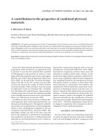
Figure 1 shows estimated heights (m) from models (1), (2),
(3), and (4) plotted against breast height age (yr) for site indices
10, 15, 20, and 25 m at breast height age 50. It appears that the
different parameter estimation techniques lead to substantially
different curves at ages above approximately 100 yr and for
higher site indices. However, the distribution of the data shows
that the curve shapes are not well-supported by data at older
ages and higher site indices. The curves for site indices 10 and
15 m have a reasonable amount of data up to and past age 150.
There is only one plot with a site index around 20 m that is older
than 125 yr. The different analysis techniques give a different
weight to the data from this plot. Therefore, the different curve
shapes are likely due to one plot. There is only one plot with a
site index around 25 m, and its age is about 75 yr. A further con-

sideration when graphically comparing curve shapes is that the
shapes are often visually different but may not be statistically
different.
Figure 2 shows the modelled height trajectories from model (5)
for the plots in the BG and ICH zones (part a) and the IDF and
PP zones (part b). This figure is split into 2 parts to illustrate a
problem with the curves for the BG and ICH zones. Although
the fit to the height trajectory for the plots in these zones was
satisfactory, the resulting model is not satisfactory. The param-
eters for the ICH zone are based on three plots, which is too
small of a sample on which to make inferences. These plots
were young and hence did not display a strong asymptotic
behaviour. This led to the curves being almost linear, and prob-
ably not accurate beyond the range of the data. The parameters
for the BG zone are based on more plots. Some of these plots
had unusual height growth patterns, but not unusual enough to
Table III. Parameter estimates and their standard errors for
model (5).
Parameter Zone(s) Estimate
Standard
error
b
0234
ICH, IDF, and PP 8.829 0.132
b
114
All 1.516 0.0207
b
12
ICH –0.4994 0.0471

b
13
IDF –0.08833 0.0119
b
21
All –2.790 0.0443
b
22
ICH 3.898 0.0753
b
234
IDF and PP 3.697 0.0653
Figure 1. Height estimates from models (1), (2), (3), and (4) plotted
against breast height age for site indices 10, 15, 20, and 25 m. This
figure shows the differences in height estimates from the four models.
Figure 2. Height estimates from model (5) plotted against breast hei-
ght age for site indices 10, 15, 20, and 25 m. This figure shows the
difference in height estimates between the four biogeoclimatic zones
that were sampled: BG and ICH – part a; IDF and PP – part b.
614 G. Nigh
invalidate their status as a site tree. The BG zone is very dry
and these height growth patterns could have been caused by site
conditions. These few plots caused the unusual height trajec-
tories for the BG zone in Figure 2a. Note that sites with a site
index of 20 or 25 m in the BG zone probably do not exist and
the curves shown in Figure 2a for site index 20 and 25 are based
on extrapolated data. Height growth in the IDF zone does not
differ much from height growth in the PP zone, particularly at
younger ages and on lower sites (Fig. 2b). The height growth
in the PP zone, however, slows faster at older ages than in the

IDF, particularly at higher site indices. The divergence of the
two curves occurs where there is little or no data. Consequently,
there is some data to support the evidence that there is a differ-
ence in the height growth patterns between the IDF and PP
zones, but the evidence is not conclusive.
Figure 3 is a comparison between model (4) and the Hann
and Scrivani [10] model. Model (4) produces lower height esti-
mates below the index age and on better sites. It has higher
heights on poorer sites above the index age. The trajectories of
the two curves are similar in the mid to high site index range,
which is likely the most important range because there are few
high sites, and harvesting and management will not be targeted
at the lower sites.
4. DISCUSSION
The BC Ministry of Forests currently recommends that the
site index models developed by Hann and Scrivani [10] be used
to estimate the height and site index of ponderosa pine in BC
This research provides an alternative model that is based on
data collected in BC using local standards for site index
research. Model (5) had the best statistical properties and had
the lowest mean squared error of the 5 models tested. However,
its height predictions are unreliable when extrapolated, espe-
cially for the BG and ICH zones. Model (4) had the smallest
mean error and its mean squared error was almost as small as
that for model (5). Therefore, I recommend the use of model (4)
for estimating the height of ponderosa pine in British Columbia.
The models cannot be algebraically inverted to predict site
index from height and age, but site index can be obtained from
the models using iterative techniques [35].
It is critically important to have good growth and yield infor-

mation for sustainable forest management of ponderosa pine
since it is not an easy species to regenerate. It is difficult to
establish because of drought at critical times in the growing season,
competing vegetation, animal damage and predation, seedling
quality, and frost heaving [11]. Natural regeneration is partic-
ularly difficult because it depends on a good seed source, ade-
quate moisture, and lack of competing vegetation all occurring
simultaneously [9]. Poor growth and yield information coupled
with the species’ regeneration difficulties may lead to unsus-
tainable forest management. This height model is a key com-
ponent for obtaining good estimates of the growth and yield of
ponderosa pine.
Four variations of the logistic model were fit to the data. In
each variation, the basic model remained the same while dif-
ferent assumptions about the error structure were modelled in
each variant. The parameter estimates changed from variant to
variant, but the shape of the curves only changed marginally,
at least within the range of the of the data.
The statistical analysis shows that height growth patterns for
ponderosa pine in the BG, ICH, IDF and PP biogeoclimatic
zones were different (Tab. III). The difference is not conclusive
for the BG and ICH zones due to a small number of plots in
these zones. The BG zone is the driest in the province and the
ICH zone is the one of the wettest and most productive in the
province [17]. Therefore, I expected that growth differences
would be more likely in these two zones. However, differing
levels of soil moisture does not necessarily impact height
growth patterns [34]. Although the curves for the IDF and PP
zones differ, the differences are small within the range of the
data (Fig. 2, and note that the divergence of the curves occurs

outside of the range of the most of the data). Overall, then, the
analysis does not conclusively show height growth differences
between biogeoclimatic zones. Model (4) is more robust and
should be used for height estimates.
The Hann and Scrivani [10] curves are similar to model (4)
(Fig. 3). When comparing the curves the range of the data must
be taken into consideration and also there are no confidence
intervals to indicate statistical differences. Discrepancies are
evident at young ages and at old ages, particularly for the high
and low sites. These are small, however, and therefore the Hann
and Scrivani curves should have given reasonable height and
site index estimates in the past.
Comparing models graphically is often done in the literature
but may lead to wrong conclusions. Conclusively detecting dif-
ferences in tree height growth between two biogeoclimatic
zones (as an example, but it may also be done for elevation or
other variables) cannot be done by plotting estimated heights
for a given level of site index, and claiming a difference if the
two lines are not identical. This method does not take into
account the natural variability in height growth patterns and
Figure 3. Height estimates from model (4) and the Hann and Scrivani
[10] model plotted against breast height age for site indices 10, 15,
20, and 25 m. This figure shows the difference in height estimates
between the two models.
Ponderosa pine height model 615
sampling error. A better comparison could be made by plotting
the confidence intervals for the two lines. However, even this
is not a rigorous procedure because the regression assumptions
in the development of the model are often violated, which leads
to biased estimates of the variance and hence biased confidence

intervals [30]. Furthermore, testing for statistical significance
using overlapping confidence intervals does not always lead to
the correct conclusion [28]. Obtaining good confidence inter-
vals for comparison or validation purposes is not easy [24]. The
other major problem with graphically comparing height trajec-
tories is that often the stem analysis data are not balanced; older
plots are usually available from poorer sites with lower site
indices. Comparing estimated height trajectories without data
to support the trajectory may be misleading. In my experience,
different model fitting techniques dramatically alters the height
trajectories beyond the range of the data [20]. Therefore, dif-
ferences in curve shapes in extrapolated ranges may be due to
the data analysis technique rather than to biological differences.
5. CONCLUSION
The height of ponderosa pine is effectively estimated from
site index and breast height age using model (4). This model is
calibrated specifically for British Columbia conditions, and in
that respect is an improvement over the Hann and Scrivani
curves, which were calibrated for southwest Oregon. However,
despite the difference in the sources of data, the two curves are
quite similar. Differences in height growth patterns between
biogeoclimatic zones were detected but not conclusive and are
small over the range of the data.
Acknowledgements: This research was funded by Forest Renewal
B.C. Dr Ken Mitchell, British Columbia Ministry of Forests, provided
helpful review comments.
REFERENCES
[1] Alexander R.R., Major habitat types, community types, and plant
communities in the Rocky Mountains, US For. Serv. Rocky Mt.
For. Range Exp. Stn. Gen. Tech. Rep. RM-123, 1985.

[2] Barrett J.W., Height growth and site index curves for managed,
even-aged stands of ponderosa pine in the Pacific Northwest,
USDA Forest Service Research Paper PNW-232, 1978.
[3] Chen H.Y.H., Klinka K., Height growth models for high-elevation
subalpine fir, Engelmann spruce, and lodgepole pine in British
Columbia, West. J. Appl. For. 15 (2000) 62–69.
[4] Chen H.Y.H., Klinka K., Kabzems R.D., Height growth and site
index models for trembling aspen (Populus tremuloides Michx.) in
northern British Columbia, For. Ecol. Manage. 102 (1998) 157–165.
[5] Daubenmire R., The use of vegetation in assessing the productivity
of forest lands, Bot. Rev. 42 (1976) 115–143.
[6] Davidian M., Giltinan D.M., Nonlinear models for repeated measu-
rement data, Chapman & Hall, London, 1995.
[7] Dolph K.L., Predicting height increment of young-growth mixed
conifers in the Sierra Nevadas, USDA Forest Service Research
Paper PSW-191, 1988.
[8] Elfving B., Kiviste A., Construction of site index equations for
Pinus sylvestris L. using permanent plot data in Sweden, For. Ecol.
Manage. 98 (1997) 125–134.
[9] Foiles M.W., Curtis J.D., Natural regeneration of ponderosa pine on
scarified group cuttings in central Idaho, J. For. 63 (1965) 530–535.
[10] Hann D.W., Scrivani J.A., Dominant-height-growth and site-index
equations for Douglas-fir and ponderosa pine in southwest Oregon,
Oregon State University, Forest Research Laboratory, Corvallis,
Oregon, Res. Bull. 59, 1987.
[11] Heidmann L.J., Ponderosa pine regeneration in the southwest, in
Foresters’ future: leaders or followers? Proceedings of the Society
of American Foresters National Convention 1985, Society of Ame-
rican Foresters, Washington, DC, 1985, pp. 228–232.
[12] Kalbfleisch J.G., Probability and statistical inference, Vol. 2, Sta-

tistical inference, Springer-Verlag Inc., New York, 1985.
[13] Klinka K., Worrall J., Skoda L., Varga P., The distribution and
synopsis of ecological and silvical characteristics of tree species of
British Columbia’s forests, Canadian Cartographics Ltd., Coquit-
lam, BC, 2000.
[14] Lloyd D., Angrove K., Hope G., Thompson C., A guide to site iden-
tification and interpretation for the Kamloops Forest Region, BC
Ministry of Forests, Research Branch, Victoria, BC Land Manage-
ment Handbook Number 23, 1990.
[15] Luttmerding H.A., Demarchi D.A., Lea E.C., Meidinger D.V.,
Vold T. (Eds.), Describing ecosystems in the field, 2nd ed., BC
Ministry of Environment, Lands and Parks, Victoria, BC, Ministry
of the Environment Manual 11, 1990.
[16] Mason R.L., Gunst R.F., Hess J.L., Statistical design and analysis
of experiments with applications to engineering and science, John
Wiley & Sons, Inc., New York, 1990.
[17] Meidinger D., Pojar J., Ecosystem of British Columbia, BC Minis-
try of Forests, Research Branch, Victoria, BC Special Report Series
Number 6, 1991.
[18] Milner K.S., Site index and height growth curves for ponderosa
pine, western larch, lodgepole pine, and Douglas-fir in western
Montana, West. J. Appl. For. 7 (1992) 9–14.
[19] Monserud R.A., Height growth and site index curves for inland
Douglas-fir based on stem analysis data and forest habitat type, For.
Sci. 30 (1984) 943–965.
[20] Nigh G.D., A Sitka spruce height-age model with improved extra-
polation properties, For. Chron. 73 (1997) 363–369.
[21] Nigh G.D., Species-independent height-age models for British
Columbia, For. Sci. 47 (2001) 150–157.
[22] Nigh G.D., Love B.A., A model for estimating juvenile height of

lodgepole pine, For. Ecol. Manage. 123 (1999) 157–166.
[23] Nigh G.D., Love B.A., Juvenile height development in interior spruce
stands of British Columbia, West. J. Appl. For. 15 (2000) 117–121.
[24] Nigh G.D., Sit V., Validation of forest height-age models, Can. J.
For. Res. 26 (1996) 810–818.
[25] Oliver W.W., Ryker R.A., Ponderosa pine, in: Burns R.M., Honkala
B.H. (Techn. Coords.), Silvics of North America, Vol. 1, Agricul-
ture Handbook 654, USDA Forest Service, Washington, DC, 1990,
pp. 413–424.
[26] Ratkowksy D.A., Nonlinear regression modeling, Marcel Dekker,
Inc., New York, 1983.
[27] SAS Institute Inc., SAS OnlineDoc
®
, Version 8, Cary, NC, 1999.
[28] Schenker N., Gentleman J.F., On judging the significance of diffe-
rences by examining the overlap between confidence intervals, Am.
Stat. 55 (2001) 182–186.
[29] Seber G.A.F., Wild C.J., Nonlinear regression, John Wiley & Sons,
Inc. Toronto, 1989.
[30] Sen A.K., Srivastava M., Regression analysis: theory, methods, and
applications, Springer-Verlag, New York, Inc., New York, 1990.
[31] Shapiro S.S., Wilk M.B., An analysis of variance test for normality
(complete samples), Biometrika 52 (1965) 591–611.
[32] Stansfield W.F., McTague J.P., Dominant-height and site-index
equations for ponderosa pine in east-central Arizona, Can. J. For.
Res. 21 (1991) 606–611.
[33] Thrower J.S., Goudie J.W., Estimating dominant height and site
index of even-aged interior Douglas-fir in British Columbia, West.
J. Appl. For. 7 (1992) 20–25.
[34] Wang G.G., Marshall P.L., Klinka K., Height growth pattern of

white spruce in relation to site quality, For. Ecol. Manage. 68
(1994) 137–147.
[35] Wang Y., Payandeh B., A numerical method for the solution of a
base-age-specific site index model, Can. J. For. Res. 23 (1993)
2487–2489.