Coastal Lagoons - Chapter 6 ppsx
Bạn đang xem bản rút gọn của tài liệu. Xem và tải ngay bản đầy đủ của tài liệu tại đây (2.31 MB, 76 trang )
Modeling Concepts
Boris Chubarenko, Vladimir G. Koutitonsky,
Ramiro Neves, and Georg Umgiesser
CONTENTS
6.1 Introduction
6.2 Numerical Discretization Techniques
6.2.1 Computational Grid
6.2.2 Control Volume Approach
6.2.3 Numerical Calculation of Advection
6.2.3.1 Spatial Approach
6.2.3.1.1 Linear Approach
6.2.3.1.2 Upstream Stepwise Approach
6.2.3.1.3 Quadratic Upwind Approach (QUICK)
6.2.3.2 Temporal Approach
6.2.4 Taylor Series Approach
6.2.4.1 Time Discretization
6.2.4.2 Spatial Discretization
6.2.5 Stability and Accuracy
6.2.5.1 Introductory Example
6.2.5.2 Stability
6.2.5.3 The Need for a Fine Resolution Grid
6.3 Pre-Modeling Analysis and Model Selection
6.3.1 Hydrographic Classification
6.3.1.1 Morphometric Parameters
6.3.1.2 Hydrological Parameters
6.3.2 Description of Forcing Factors
6.3.2.1 General Hierarchy of Driving Forces
6.3.2.2 Water Budget Components
6.3.2.2.1 Surface Evaporation Budget
6.3.2.2.2 Ocean–Lagoon Exchange Budget
6.3.2.3 Heat Budget
6.3.3 Pre-Estimation of Spatial and Temporal Scales
6.3.3.1 Flushing Time
6.3.3.1.1 Integral Flushing Time
6.3.3.1.2 Local Flushing Time
6.3.3.2 Surface and Bottom Friction Layers
6.3.3.3 Time Scales of Current Adaptation
6
L1686_C06.fm Page 231 Monday, November 1, 2004 3:39 PM
© 2005 by CRC Press
6.3.3.3.1 Wind Driven Current
6.3.3.3.2 Equilibrium Current Structure
6.3.3.3.3 Gradient Flow Development
6.3.3.4 Wind Surge
6.3.3.5 Seiches or Natural Oscillations of a Lagoon Basin
6.3.3.6 Wind Waves
6.3.3.7 Coriolis Force Action
6.3.4 Objectives of Modeling
6.3.5 Recommendations for Model Selection
6.3.5.1 Selection Possibilities for Hydrodynamic
and Transport Models
6.3.5.2 Possible Simplifications in Spatial Dimensions
6.3.5.3 Possible Simplification in the Physical Approach
6.3.5.4 Possible Simplification According to the Task
To Be Solved
6.3.5.5 Computer, Data, and Human Resources
6.4 Model Implementation
6.4.1 Bathymetry and the Computational Grid
6.4.1.1 Laterally Integrated Models
6.4.1.2 Horizontal Resolution Models
6.4.2 Initial Conditions
6.4.3 Boundary Conditions
6.4.4 Internal Coefficients: Calibration and Validation
6.5 Model Analysis
6.5.1 Model Restrictions
6.5.1.1 Physical Restrictions
6.5.1.2 Numerical Restrictions
6.5.1.3 Subgrid Processes Restrictions
6.5.1.4 Input Data Restrictions
6.5.2 Sensitivity Analysis
6.5.3 Calibration
6.5.4 Validation
Acknowledgments
References
Note:
The term
modeling
is used in this chapter in the sense of “numerical
modeling.” Physical modeling, conceptual modeling, or numerical model-
ing will only be used explicitly in relevant cases.
6.1 INTRODUCTION
In Chapter 3, the concept of transport equation was introduced, starting from the
concepts of control volume and accumulation rate of a property inside this control
volume. Diffusive and advective fluxes were also defined to account for exchanges
between the control volume and its neighborhood, and the concept of evolution equation
was introduced by adding sources and sinks to the transport equation. A “model” is
L1686_C06.fm Page 232 Monday, November 1, 2004 3:39 PM
© 2005 by CRC Press
built on the same concepts. Its implementation requires the definition of at least one
control volume, the calculation of the fluxes across its boundary, and the calculation of
the source and sinks using values of the state variables inside the volume. The number
of dimensions of the model depends on the importance of relevant property gradients.
The simplest model is the “zero-dimensional” model. In this model, there is no
spatial variability, and only one control volume needs to be considered. At the other
extreme of complexity is the three-dimensional (3D) model, which is required when
properties vary along the three spatial dimensions. Whatever the number of its
dimensions, a model must include the following elements:
• Equations
• Numerical algorithm
• Computer code
The order of the items in this list can also be considered the order of their chrono-
logical development. Hydrodynamic equations are based on mass, momentum, and
energy conservation principles, which were presented in Chapter 3. These have been
known for more than 100 years. Actually, numerical algorithms used to solve hydro-
dynamic models were attempted even before the existence of computers. The analytical
equations and the numerical algorithms developed before the existence of computers
allowed the rapid development of modeling starting in the 1960s, when computers were
made available to a small scientific community. Since that time, models and the mod-
eling community have evolved exponentially. Modern integrated computer codes have
done more for interdisciplinarity than 100 years of pure field and laboratory work.
The number of implementations of a model to solve various problems increases
the knowledge of the range of validity of the model equations. The accuracy of the
numerical algorithm is better known and confidence in the results increases. At that
time, the major source of errors in the results is the existence of mistakes in the data
files. Once the model equations, algorithms, and results are validated, the next priority
is the development of a user-friendly graphical interface that simplifies the use of the
model by nonspecialists. This reduces the errors of input files and simplifies the checking
of those files. This chapter presents the concepts and methodologies used to build models
and to understand their functioning.
6.2 NUMERICAL DISCRETIZATION TECHNIQUES
Computers can solve only algebraic equations. Analytic equations, integral or dif-
ferential, must be discretized into algebraic forms. The procedure followed depends
on the form of the analytical equation to be solved. The control volume approach
is best for the integral form of evolution equations, while the Taylor series is best
suited for differential equations.
6.2.1 C
OMPUTATIONAL
G
RID
The calculation of fluxes across a control volume surface is simpler if the scalar
product of the velocity by the normal to each elementary area (face) composing that
L1686_C06.fm Page 233 Monday, November 1, 2004 3:39 PM
© 2005 by CRC Press
surface remains constant in each of them. The control volume that makes that
calculation simpler must have faces perpendicular to the reference axis. If rectangular
coordinates are used, the control volume generating the simpler discretization is a
parallelepiped. In the case of a large oceanic model, a suitable control volume will
have faces laying on meridians and parallels.
In depth-integrated models, also called two-dimensional or 2D horizontal mod-
els, the upper face of the control volume is the free surface and the lower face is
the bottom. In three-dimensional or 3D models, a control volume occupies only part
of the water column and its shape depends on the vertical coordinate used. In coastal
lagoons, Cartesian and sigma-type coordinates (or a combination of both) are the
most commonly used coordinates.
The ensemble of all control volumes forms the computational grid. In finite-
difference-type grids, control volumes are organized along spatial axes and a struc-
tured grid is obtained. In contrast, typical finite-element grids are nonstructured. The
latter are more difficult to define, but they are more flexible, thus allowing some
variability in the spatial resolution. Figure 6.1 shows an example of a very general
finite-difference-type grid using several discretizations in the vertical direction.
A system can be considered one-dimensional (1D) if properties change only
along one physical dimension. In this case, control volumes can be aligned along
the line of variation and one spatial coordinate is enough to describe their locations.
Properties are considered as being constants across control volume faces perpendic-
ular to that axis. Fluxes across the faces not perpendicular to that axis are null or
have no net resultant.
6.2.2 C
ONTROL
V
OLUME
A
PPROACH
Control volumes used in numerical models have the same meaning as the derivation
of the evolution equation in Chapter 3. A discretization is adequate if it generates a
simple calculation algorithm while maintaining the accuracy of the results. The
FIGURE 6.1
Example of a grid for a three-dimensional (3D) computation. Two vertical
domains are used. The upper domain uses a sigma coordinate. The lower one uses a Cartesian.
L1686_C06.fm Page 234 Monday, November 1, 2004 3:39 PM
© 2005 by CRC Press
simpler calculation is obtained if properties can be considered as being constant inside
the control volume and along parts of its surface. To make this possible without com-
promising accuracy, the control volume must be as small as possible; a fine-resolution
grid is needed.
In a 1D model, properties can be stored into 1D arrays (vectors). Adjacent
elements of a generic element
i
are
i
– 1 on the left side and
i
+
1 on the right
side (Figure 6.2). The length of a control volume must be small enough to allow
properties in its interior to be represented by the value at its center. In that case,
equations deduced in Section 3.2 apply and the rate of accumulation in volume
i
will
be given by
where
∆
t
is the time step of the model. This equation is simplified if the volume
remains constant in time. This is not the case in most coastal lagoons subjected to
changing winds and it is certainly not the case in tidal lagoons.
Exchanges between
i
volume and neighboring ones are accounted for by advec-
tive and diffusive fluxes. Their calculation requires some hypotheses. Let us consider
Figure 6.2 and define the distances between the faces (spatial step) and the location
points where other auxiliary variables are defined as shown in Figure 6.3. The net
advective gain of matter to volume
i
is given by
where while the diffusive flux, using the approach of Chapter 3, is
given by
FIGURE 6.2
Example of one-dimensional (1D) grid.
V
i
V
i−1
V
i+1
Accumulation Rate =
−
+
() ()VC VC
t
ii
tt
ii
t∆
∆
QC QC
ii
i
i
tt
−− ++
=
−
()
1
2
1
2
1
2
1
2
*
QuA
iii−−−
=
1
2
1
2
1
2
−
()
−
+
+
()
−
+
−
−
−
−
=
++
+
+
=
νν
i
i
ii
ii
tt
ii
ii
ii
tt
A
CC
xx
A
CC
xx
1
2
1
2
1
2
1
2
1
1
2
1
1
1
2
1
() ()
**
∆∆ ∆∆
L1686_C06.fm Page 235 Monday, November 1, 2004 3:39 PM
© 2005 by CRC Press
In these equations,
t
*
is a time interval between
t
and
t
+ ∆
t
, to be defined
according to criteria outlined in the next paragraph. is the concentration on
the interface between elements
i
and
i
– 1 and will be specified later. Combining
the three equations, we obtain:
(6.1)
In order to introduce the Taylor series discretization methods and to analyze
stability and accuracy concepts, let us consider a simplified version of Equation (6.1).
Consider the particular case of a channel with uniform and permanent geometry and
regular discretization. The cross section (
A
), volume (
V
), and discharge are constant.
Assume that diffusivity can be considered constant. Under these conditions,
Equation (6.1) becomes
(6.2)
where
U
is the constant cross-section average velocity and
∆
x
is the ratio between
the volume and the average cross section. This is the most popular form of the
transport equation but, as shown above, it is applicable only to particular conditions.
Additional approaches are required to calculate the advective flux, because the
concentration is defined at the center of the control volumes and not at the faces. These
approaches and their numerical consequences are described in the next sections.
FIGURE 6.3
Generic control volume in a 1D discretization.
C
i−1
C
i
C
i+1
V
i+1
V
i
V
i−1
Q
i−
1
/
2
Q
i+
1
/
2
ν
i−
1
/
2
ν
i−
1
/
2
A
i−
∆x
i−1
A
i+
1
/
2
∆x
i+1
∆x
i
1
/
2
C
i−
1
2
() ()
() (
*
*
VC VC
t
QC QC
A
CC
xx
A
CC
x
ii
tt
ii
t
ii ii
tt
i
i
ii
ii
tt
ii
ii
i
+
−− ++
=
−
−
−
−
=
++
+
−
=−
()
−
()
−
+
+
()
−
∆
∆
∆∆ ∆
1
2
1
2
1
2
1
2
1
2
1
2
1
2
1
2
1
1
2
1
1
1
2
νν
++
+
=
∆x
i
tt
1
)
*
CC
t
U
CC
x
CCC
x
i
tt
i
t
ii
tt
iii
tt
+
−+
=
−+
=
−
=
−
+
−+
∆
∆∆ ∆
1
2
1
2
11
2
2
*
*
ν
L1686_C06.fm Page 236 Monday, November 1, 2004 3:39 PM
© 2005 by CRC Press
6.2.3 N
UMERICAL
C
ALCULATION
OF
A
DVECTION
6.2.3.1 Spatial Approach
Three common approaches are used to estimate concentration values at control
volume faces:
• Linear approach
• Upstream stepwise approach
• Quadratic upwind approach (QUICK)
6.2.3.1.1 Linear Approach
In the linear approach it is assumed that:
Assuming a discretization where the grid size is uniform, it is easily seen that this
approach generates central differences as obtained using the Taylor series (see
Section 6.2.4).
6.2.3.1.2 Upstream Stepwise Approach
In this case, it is assumed that the concentration at the left face is
This discretization respects the transportivity property of advection. This property
states that advection can transport properties only downstream or that information
comes only from upstream. The linear approach does not respect this property
because volume
i
will get information of downstream concentration through the
average process. The violation of this property can generate instabilities and will
create conditions to obtain negative values of the concentration. The upstream
discretization avoids this limitation but, as shown in the following paragraphs, it can
introduce unrealistic numerical diffusion.
6.2.3.1.3 Quadratic Upwind Approach (QUICK)
The quadratic upwind approach, or QUICK scheme, is an attempt at a compromise
between respecting the transportivity property and keeping numerical diffusion at
low values. In this case, it is assumed that the concentration distribution around a
point follows a quadratic distribution centered on the upstream side of the face
C
Cx C x
xx
i
ii i i
ii
−
−−
−
=
+
+
1
2
11
1
∆∆
∆∆
QCC
QCC
iii
iii
>⇒ =
()
<⇒ =
()
−
−
−
0
0
1
2
1
2
1
L1686_C06.fm Page 237 Monday, November 1, 2004 3:39 PM
© 2005 by CRC Press
being calculated. For the left face, we obtain
Using the Taylor series discretization described in the next paragraph, it can be
seen that, in the case of a regular discretization, advection calculated using this
approach is third-order accurate,
1
while pure upstream discretization is first-order
accurate and the linear approach (central differences) is second-order accurate. The
inconvenience of the QUICK discretization is that it requires additional approaches
close to the boundaries. This is not a very limiting factor in 1D calculation but it is
in 2D or 3D calculations, especially when the geometry is irregular.
6.2.3.2 Temporal Approach
In previous paragraphs, spatial discretization was analyzed. A solution was described
for the diffusion term and three discretizations were suggested for the advection
term but nothing was said about the time level at which the variables used to calculate
advection or diffusion are evaluated. Figure 6.4 shows an example of a time evolution
of a property
C
at a point. The curved line shows the continuous evolution and filled
circles show values at each time step. Vertical arrows show
C
values at the beginning
and end of a particular time step
∆
t
. The flux in that time step is proportional to the
product
∆
C
∆
t
. Values at the beginning and end of a time step are shown, as well as
concentration variation during that time step. The rate of accumulation at this point
is proportional to the slope of this line. The slope of this line also gives an idea of
the errors associated with the choice of
t
*
.
FIGURE 6.4
Visualization of the consequences of temporal discretization. Property evolves
within a time step, but values used to calculate flux do not.
Time
Property value
∆C
∆t
0
140
QCCCC
QCCCC
iiiii
iiiii
>⇒ = + −
()
<⇒ = + −
()
−
−−
−
−+
0
0
1
2
1
2
6
8
1
3
8
1
8
2
6
8
3
8
1
1
8
1
L1686_C06.fm Page 238 Monday, November 1, 2004 3:39 PM
© 2005 by CRC Press
Models with
explicit
numerical schemes
use
t
*
=
t
, while models with
implicit
schemes consider
t
*
=
t
+ ∆
t.
It can be seen from the figure that when the slope of
the curve is positive, explicit models underestimate the advective fluxes,
†
while when
the slope is negative, they overestimate them, introducing (at least) a phase error.
Implicit schemes, on the other hand, underestimate or overestimate the fluxes by a
value of the same order. The consideration of an intermediate value between
t
and
t
+ ∆
t
generates more accurate fluxes. The next subsection shows that
t
*
=
t
+
1
/
2
∆
t
(semi-implicit method) gives the maximum accuracy. Values at
t
*
=
t
+
1
/
2
∆
t
can
be obtained by averaging the values of the properties calculated at time
t
and time
t
+ ∆
t. An increasing number of calculations to perform is the price to pay for
accuracy improvement.
The next subsection shows that implicit methods have better stability properties
than explicit methods. It can be shown that stability properties of the semi-implicit
methods are similar to those of implicit methods. Because of their stability and accu-
racy properties, semi-implicit methods are the most efficient numerical methods.
6.2.4 TAYLOR SERIES APPROACH
Traditionally, discretized equations are obtained from partial differential equations
by replacing derivatives with finite-differences obtained using the Taylor series. The
Taylor series provides information on the truncation errors arising when replacing
derivatives by finite-differences. In contrast, the control volume introduced in the
previous subsection gives information about physical approaches used during dis-
cretization. When applied correctly, both methods must produce the same discretized
equations.
In order to introduce the Taylor series discretization methods and to analyze
stability and accuracy concepts, let us consider the differential equation correspond-
ing to Equation (6.2):
(6.3)
This equation describes the advection–diffusion transport in a channel with uniform
velocity, a permanent geometry, and diffusivity.
6.2.4.1 Time Discretization
The Taylor series relates the value of a property in a point (or time instant) with the
values of the property in another point and the derivatives in the same point:
†
In explicit methods the flux during a time step is proportional to the area of the rectangle with side
lengths ∆t and C
t
, while in implicit methods it is proportional to ∆t and C
t+∆t
.
∂
∂
+
∂
∂
=
∂
∂
C
t
U
C
x
C
x
ν
2
2
CC t
C
t
tC
t
tC
t
t
n
C
t
t
i
tt
i
t
i
t
i
t
i
t
nn
n
i
t
n+ +
=+
∂
∂
+
∂
∂
+
∂
∂
++
∂
∂
+
∆
∆
∆∆ ∆
∆
22
2
33
3
1
23
0
!!
()L
L1686_C06.fm Page 239 Monday, November 1, 2004 3:39 PM
© 2005 by CRC Press
Truncating this series at the first derivative, we obtain
(6.4)
This equation states that the resolution of all the terms of the equation at time t
allows the calculation of the variable at time t +∆t with first-order precision because
the first missing term in the series is multiplied by ∆t.
Similarly, we can relate the concentration at time t with the concentration at
time t + ∆t:
Truncating this series after the first derivative as before, we obtain
(6.5)
This equation shows that in implicit methods the truncation error is also of the
first order, as in explicit methods, although processes are computed at time t + ∆t.
The difference between implicit and explicit methods is their stability properties, as
described in the following.
From the above paragraph, it is expected that explicit and implicit methods
should have the same truncation error and it is also expected that the calculation of
the derivatives (or fluxes) at the center of the time step must have a smaller truncation
error. To demonstrate this, let us use the Taylor series to relate properties at time and
with variables at .
(6.6)
Subtracting the second equation from the first equation, we obtain
∂
∂
=
−
+
+
C
t
CC
t
Ot
i
t
i
tt
i
t∆
∆
∆()
CC t
C
t
tC
t
tC
t
t
n
C
t
t
i
t
i
tt
i
tt
i
tt
i
tt
nn
n
i
tt
n
=−
∂
∂
+
∂
∂
−
∂
∂
++
∂
∂
+
+
+
++
+
+
∆
∆
∆∆
∆
∆
∆∆
∆
∆
22
2
33
3
1
23
0
!
!
()L
∂
∂
=
−
+
+
+
C
t
CC
t
t
i
tt
i
tt
i
t
∆
∆
∆
∆0( )
t
tt+∆ tt+∆/2
CC
t
C
t
t
C
t
t
CC
t
C
t
t
C
i
tt
i
tt
i
tt
i
tt
i
t
i
tt
i
tt
++
+
+
+
+
=+
∂
∂
+
()
∂
∂
+
()
=−
∂
∂
+
()
∂
∆∆
∆
∆
∆
∆
∆
∆
∆
∆
∆
/
/
/
/
/
2
2
2
2
2
2
3
2
2
2
2
2
2
2
0
2
2
2
2 ∂∂
+
()
+
t
t
i
tt
2
2
3
0
2
∆
∆
/
∂
∂
=
−
+
()
+
+
C
t
CC
t
t
i
tt
i
tt
i
t
∆
∆
∆
∆
/2
2
0
2
L1686_C06.fm Page 240 Monday, November 1, 2004 3:39 PM
© 2005 by CRC Press
This equation shows that semi-implicit methods are second-order accurate, and
consequently allow for use of larger time step values. The implementation of these
methods requires the computation of all derivatives and fluxes centered in time.
Those values also can be computed with second-order accuracy, as the average
between values at time and , and can be demonstrated using expansions from
Equation 6.6:
This temporal semi-implicit discretization is known as the Crank-Nicholson discret-
ization. In this discretization we get
In order to solve this equation, the spatial derivatives have to be discretized.
6.2.4.2 Spatial Discretization
Spatial discretization using the Taylor series follows an approach similar to temporal
discretization. Let us consider Taylor series developments for points on the left and
on the right of point i, at a distance at an arbitrary time level:
(6.7)
(6.8)
Subtracting Equation (6.8) from Equation (6.7), we get the so-called central differ-
ence for the first-order spatial derivative of C:
(6.9)
From Equation (6.7), we obtain an expression for a noncentered derivative (right
side derivative), while from Equation (6.8), we obtain a left-side derivative, both
with a first-order truncation error:
(6.10)
(6.11)
t tt+∆
C
CC
t
i
tt
i
t
i
tt
+
+
=
+
+
∆
∆
∆
/
()
22
2
0
CC
t
U
C
x
C
x
U
C
x
C
x
t
i
tt
i
t
i
tt
i
t
+
+
−
=−
∂
∂
+
∂
∂
+−
∂
∂
+
∂
∂
+
∆
∆
∆
∆
1
2
1
2
0
2
2
2
2
2
νν
()
∆x
CC x
C
x
xC
x
xC
x
x
ii
i
ii
+
=+
∂
∂
+
∂
∂
+
∂
∂
+
1
22
2
33
3
3
23
0
**
*
**
!
()∆
∆∆
∆
CC x
C
x
xC
x
xC
x
x
ii
i
ii
−
=−
∂
∂
+
∂
∂
−
∂
∂
+
()
1
22
2
33
3
3
23
0
**
*
**
!
∆
∆∆
∆
∂
∂
=
−
+
+−
C
x
CC
x
x
i
ii
*
**
()
11
2
2
0
∆
∆
∂
∂
=
−
+
+
C
x
CC
x
x
i
ii
*
**
()
1
0
∆
∆
∂
∂
=
−
+
−
C
x
CC
x
x
i
ii
*
**
()
1
0
∆
∆
L1686_C06.fm Page 241 Monday, November 1, 2004 3:39 PM
© 2005 by CRC Press
If Equation (6.10) is used when the velocity is negative and Equation (6.11) is used
when the velocity is positive, the first derivative is computed using an “upstream
method,” since in both cases no downstream information is used.
Adding Equation (6.7) and Equation (6.8), we obtain
(6.12)
which is the finite-difference form of the second spatial derivative, discretized with
a second-order truncation order.
In the next subsection, the stability criteria for some of these discretizations are
analyzed. It will be shown that central differences for first-order derivatives generate
unstable algorithms, and it will be shown that truncation error is not the unique
aspect to take into account for estimating the accuracy of a numerical algorithm.
6.2.5 STABILITY AND ACCURACY
6.2.5.1 Introductory Example
The exponential decay equation is considered first as an example because it illustrates
the main features of stability without having to deal with spatial derivatives. This
differential equation reads
(6.13)
where C is a generic concentration and
α
is a positive constant. The analytical solution
to this problem is
where is the initial concentration at time . If the previous equation is
discretized in time, we obtain
As explained previously, we still must decide at which time level the term on
the right-hand side has to be evaluated. Starting with an explicit approach, such that
, we can solve the equation directly for C at the new time level:
∂
∂
=
−+
+
+−
2
2
11
2
2
2
0
C
x
CCC
x
x
i
iii
*
***
()
∆
∆
∂
∂
=−
C
t
C
α
CC t=−
0
exp( )
α
C
0
t = 0
CC
t
C
tt t
t
+
−
=−
∆
∆
()
*
α
tt
*
=
CC tC tC
tt t t t+
=− =−
∆
∆∆
αα
()1
L1686_C06.fm Page 242 Monday, November 1, 2004 3:39 PM
© 2005 by CRC Press
As long as is small (more precisely ), the solution is approximating
the exponential decay. But once becomes equal to , the solution reads:
and so, in the first time step, the value of the concentration drops to 0 and then stays
there. Even worse, if then and concentrations become nega-
tive, a completely nonphysical behavior.
However, even with these negative values, the solution of the decay equation is
still stable because the oscillations generated are slowly decaying. However, if has
been chosen to be , then , and the oscillations start to
amplify instead of decaying. There is no mechanism to dampen these oscillations
and so they will amplify to reach arbitrary large (positive and negative) values. The
solution has become unstable.
This behavior is shown in Figure 6.5 where the solution to the decay equation
with has been plotted. As can be seen, all solutions with a time step of less
than 1 are stable and are not undershooting. The solution with drops to 0 in
the first time step, whereas for the solution produces negative values, but
the solution is still stable. Finally, for the solution becomes unstable.
The situation changes completely when the implicit approach is used. Now the
discretized equation reads
or, after solving for the concentration on the new time level,
FIGURE 6.5 Solution of the decay equation (Equation (6.13)) with the explicit scheme with
different time steps.
Explicit scheme, α = 1
−150
−100
−50
0
50
100
150
024681012
time
concentration
analytical solution
time step 0.1
time step 0.5
time step 1.0
time step 1.5
time step 2.1
∆t
α
∆t <1
∆t
1/
α
CC
i
tt
i
t+
==
∆
()00
∆t > (/ )1
α
()10−<
α
∆t
∆t
∆t > (/ )2
α
()11−<−
α
∆t
α
=
1
∆t = 1
∆t = 15.
∆t = 21.
CC tC
tt t tt++
=−
∆∆
∆
α
C
t
C
tt t+
=
+
∆
∆
1
1
α
L1686_C06.fm Page 243 Monday, November 1, 2004 3:39 PM
© 2005 by CRC Press
As can be seen, this solution does not become unstable for any time step. The
concentrations will always remain positive and no undershoots will occur. This is
the desired property for the solution to the decay equation. Please note that the
implicit solutions all have higher values than the analytical solution, whereas the
stable and physical meaningful explicit solutions are all smaller than the analytical
one. The solutions for the implicit scheme can be seen in Figure 6.6.
If the growth equation is considered instead of the decay equation, all arguments
change. The growth equation reads
Clearly this equation can be reproduced by the decay equation just by setting
α
to
a negative value.
As can be seen easily, the growth equation remains stable if an explicit scheme
is used. However, if an implicit scheme is used, the solution will be stable only if
β
satisfies the stability criterion derived for
α
.
In summary, it seems clear that for the decay equation, we should always use
an implicit scheme in order to have a situation where solutions are stable for every
time step used. On the other hand, if the growth equation is to be solved, an explicit
scheme is better for the stability of the model.
The stability and accuracy associated with different options for temporal and
spatial discretizations of the advection and diffusion equations (Equation (6.2)) can
be examined by considering central explicit differences in the particular case of no
FIGURE 6.6 Solution of the decay equation (Equation (6.13)) with the implicit scheme with
different time steps.
Implicit scheme, a = 1
0
20
40
60
80
100
120
024681012
time
concentration
analytical solution
time step 0.1
time step 0.5
time step 1.0
time step 1.5
time step 2.1
∂
∂
=
C
t
C
β
L1686_C06.fm Page 244 Monday, November 1, 2004 3:39 PM
© 2005 by CRC Press
diffusion. In that case Equation (6.2) becomes
(6.14)
where is the Courant number representing the ratio between the path length
of a particle during a time step and the grid size. This is a critical parameter for
most discretizations. Let us consider the case of a channel where initial conditions
are zero everywhere except in a generic point i. Table 6.1 shows the temporal
evolution along 11 time steps (0 to 11) for the case of a unitary Courant number
(C
r
= 1) and Table 6.2 shows the corresponding solution for the case of C
r
= 2.
In both tables, columns i – 3 and i + 3 represent the boundary conditions (zero
outside of the modeling area) and total amount stands for the total amount of matter
inside the channel. Both solutions are unrealistic.
In such conditions, one would expect the contaminated water to move forward
and, after a certain time, the entire channel should have a concentration equal to
zero because the water entering the model area has concentration zero. The value
of the total amount of matter inside the channel should remain constant until the
matter reaches the outflow boundary, and then drop to zero while it leaves the domain.
6.2.5.2 Stability
A model is said to be unstable if errors generated inside the modeling area are
amplified. This is what has happened in both the calculations. As time increased,
TABLE 6.1
Example of a Time Evolution in a 1D Channel Computed Using Explicit
Central Differences, a Unitary Courant Number, and No Diffusion
Time Step
Grid Point Number
Total Amount
i – 3 i – 2 i – 1 ii
+ 1 i + 2 i + 3
0 00 0100 0 1
1 0 0.00 –0.50 1.00 0.50 0.00 0 1
2 0 0.25 –1.00 0.5 1.00 0.25 0 1
3 0 0.75 –1.13 –0.50 1.13 0.75 0 1
4 0 1.31 –0.50 –1.63 0.50 1.31 0 1
5 0 1.56 0.97 –2.13 –0.97 1.56 0 1
6 0 1.08 2.81 –1.16 –2.81 1.08 0 1
7 0 –0.33 3.93 1.66 –3.93 –0.33 0 1
8 0 –2.29 2.94 5.59 –2.94 –2.29 0 1
9 0 –3.76 –1.00 8.52 1.00 –3.76 0 1
10 0 –3.26 –7.14 7.52 7.14 –3.26 0 1
11 0 0.31 –12.54 0.38 12.54 0.31 0 1
CC
t
U
CC
x
C
Ut
x
CC
Ut
x
C
i
tt
i
t
ii
t
i
tt
i
t
i
t
i
t
+
−+
+
−−
−
=
−
=+−
∆
∆
∆∆
∆
∆
∆
∆
11
11
2
1
2
1
2
Ut
x
C
r
∆
∆
=
L1686_C06.fm Page 245 Monday, November 1, 2004 3:39 PM
© 2005 by CRC Press
the errors have increased. The error growth rate has been higher at a higher Courant
number. To understand the reasons for such instability, we can use the following
principle:
“The influence of a point on its neighbors through advection or diffusion cannot be
negative.”
This means that the consequence of increasing the concentration in one point
can never be a reduction in any of its neighboring points. In order to guarantee
the respect of this principle, no coefficient of the grid point values in Equation
(6.14) can be negative. If a coefficient is null, there is no influence. In Equation
(6.14), the coefficient of C
i+1
is negative whatever the Courant number. As a
consequence, the higher the concentration in that point, the smaller the concen-
tration in point i.
This method can be stabilized by adding diffusion. For example, if diffusion is
considered, Equation (6.14) becomes
(6.15)
TABLE 6.2
Example of a Time Evolution in a 1D Channel Computed Using Explicit Central
Differences, C
r
= 2, and No Diffusion
Time Step
Grid Point Number
Total
Amounti – 3 i – 2 i – 1 ii
+ 1 i + 2 i + 3
0 0 0 0 1 0 0 0 1
1 0 0.00 –1.00 1.00 1.00 0.00 0 1
2 0 1.00 –2.00 –1.00 2.00 1.00 0 1
3 0 3.00 0.00 –5.00 0.00 3.00 0 1
4 0 3.00 8.00 –5.00 –8.00 3.00 0 1
5 0 –5.00 16.00 11.00 –16.00 –5.00 0 1
6 0 –21.00 0.00 43.00 0.00 –21.00 0 1
7 0 –21.00 –64.00 43.00 64.00 –21.00 0 1
8 0 43.00 –128.00 –85.00 128.00 43.00 0 1
9 0 171.00 0.00 –341.00 0.00 171.00 0 1
10 0 171.00 512.00 –341.00 –512.00 171.00 0 1
11 0 –341.00 1024.00 683.00 –1024.0 –341.00 0 1
CC
t
U
CC
x
CCC
x
C
Ut
x
t
x
C
t
x
C
Ut
x
t
x
i
tt
i
t
ii
t
iii
t
i
tt
i
t
i
t
+
−+ − +
+
−
−
=
−
+
−+
=+
+−
+− +
∆
∆
∆∆ ∆
∆
∆
∆
∆
∆
∆
∆
∆
∆
∆
11 1 1
2
2
1
22
2
1
2
12
1
2
ν
νν ν
+
C
i
t
1
L1686_C06.fm Page 246 Monday, November 1, 2004 3:39 PM
© 2005 by CRC Press
where is called the diffusion number. In this case, positiveness of the coef-
ficients is assured if
(6.16)
with Re
g
being the grid Reynolds number. The consideration of advection alone is
equivalent to the consideration of an infinite Reynolds number and, consequently, what-
ever the time step (or C
r
), central differences are always unstable. If on the one hand it
is important for stability that v is high enough (Equation (6.16a)), on the other hand it
is limited by Equation (6.16b) and may not exceed a critical value given by d ≤ 1/2.
The consideration of diffusion does not always increase the stability properties
of numerical models. Why did it in this case? Central differences do not respect the
transportive property of advection. Physically, advection can only propagate infor-
mation in the direction of the velocity. The analysis of Table 6.1 and Table 6.2 shows
that information has also been propagated backward. This was a consequence of the
use of a downstream value (C
i +1
) to calculate the spatial derivative. Physically,
diffusion propagates the information in any direction (according to the local gradi-
ents). In the case of Table 6.1 and Table 6.2, information diffusion transports matter
upstream, making it available to be transported by advection.
When the advective flux is calculated using downstream information, one can
remove matter from a control volume that is not to be removed. This is the mechanism
that generates negative concentrations. The method is unstable because those errors are
amplified in time. The consideration of (enough) diffusion makes the method stable but
does not avoid the generation of negative concentrations. The upstream discretization
was proposed first to avoid this problem. Consider now upstream explicit differences
and again the particular case of no diffusion. In this case, Equation (6.2) becomes
(6.17)
It is easy to verify that the method is stable if the Courant number is not greater
than 1. Table 6.3 shows results for C
r
= 1 and Table 6.4 shows results for C
r
= 0.5.
C
r
> 1 would generate an unstable model, which could not be solved adding diffusion.
In fact, if diffusion were considered, the stability criteria would be (C
r
+ 2d) ≤ 1.
Table 6.3 shows that explicit upstream differences with C
r
= 1 give the exact
result. The concentration remains constant and travels at the exact speed of 1 cell
per iteration. When the Courant number is reduced to 0.5 (Table 6.4) the solution
is however degradated through the introduction of numerical diffusion. The method
remains stable because the errors are reduced in time.
The results obtained in the above four examples show that small truncation errors
as given by the Taylor series are not enough to guarantee accurate results. The
upstream results also show that the reduction of the time step does not guarantee an
improvement of the results.
ν
∆
∆
t
x
d
2
=
Re
g
Ux
d
vt
x
=≤
=≤
∆
∆
∆
ν
2
1
2
2
C
Ut
x
C
Ut
x
CU
i
tt
i
t
i
t+
−
=+−
>
∆
∆
∆
∆
∆
1
10()
L1686_C06.fm Page 247 Monday, November 1, 2004 3:39 PM
© 2005 by CRC Press
6.2.5.3 The Need for a Fine Resolution Grid
The reason why the upstream scheme with C
r
= 0.5 gives such poor results is the
coarse discretization used. In this case, matter travels only half of the grid size and
consequently the matter contained in cell i at t = 0 is distributed between two
computing cells at time t = 1. Because the concentration is computed as the mass
divided by the volume, its value is reduced to
1
/
2
. This result is obtained because
the initial hypothesis that “the grid cell is small enough to allow the concentration
TABLE 6.3
Example of a Time Evolution in a 1D Channel Computed Using
Explicit Upstream Differences, C
r
= 1.0, and No Diffusion
Time Step
Grid Point Number
Total Amounti – 3 i – 2 i – 1 ii
+ 1 i + 2 i + 3
0 0001 0 0 0 1
1 0000 1 0 0 1
2 0000 0 1 0 1
3 0000 0 0 0 0
4 0000 0 0 0 0
5 0000 0 0 0 0
6 0000 0 0 0 0
7 0000 0 0 0 0
8 0000 0 0 0 0
9 0000 0 0 0 0
10 0000 0 0 0 0
TABLE 6.4
Example of a Time Evolution in a 1D Channel Computed Using Explicit
Upstream Differences, C
r
= 0.5, and No Diffusion
Grid Point Number
Time Step i – 3 i – 2 i – 1 ii
+ 1 i + 2 i + 3 Total Amount
0 0 001 0 0 0 1
1 0 0.00 0.00 0.50 0.50 0.00 0 1
2 0 0.00 0.00 0.25 0.50 0.25 0 1
3 0 0.00 0.00 0.13 0.38 0.38 0 0.88
4 0 0.00 0.00 0.06 0.25 0.38 0 0.69
5 0 0.00 0.00 0.03 0.16 0.31 0 0.5
6 0 0.00 0.00 0.02 0.09 0.23 0 0.34
7 0 0.00 0.00 0.01 0.05 0.16 0 0.23
8 0 0.00 0.00 0.00 0.03 0.11 0 0.14
9 0 0.00 0.00 0.00 0.02 0.07 0 0.09
10 0 0.00 0.00 0.00 0.01 0.04 0 0.05
L1686_C06.fm Page 248 Monday, November 1, 2004 3:39 PM
© 2005 by CRC Press
to be uniform in its interior” is violated. This does not happen when half of the cell
has matter and the other half does not. If the plume were contained inside many
cells the problem would still exist but only in the plume limits and hence would not
deteriorate the solution.
6.3 PRE-MODELING ANALYSIS AND MODEL SELECTION
6.3.1 H
YDROGRAPHIC CLASSIFICATION
Characteristics of lagoons around the world are very different. Geomorphological
characteristics depend on the type of shore, while hydrological characteristics
are determined by marine influence and hydrological balance for the lagoon
drainage basin. Lagoons with similar morphometry may exhibit completely dif-
ferent behavior in different ambient conditions. A careful classification of the
lagoon type according to its geomorphology, hydrology, and mixing processes is
a desirable first step toward the choice of the most appropriate physics to be
included in the numerical model. The proper identification of a lagoon type allows
the user to find a similar lagoon in another part of the world and benefit from
the previous knowledge available for that lagoon. At the same time, the hydro-
graphic classification database will be supplemented with new information that
can be used for future studies in similar lagoons. It is very tempting to classify
a lagoon according to its hydrographic features, i.e., utilizing only basic infor-
mation on its morphometry and hydrology, which is usually available without
additional field studies.
A proper lagoon, such as an atoll lagoon or a coastal lagoon (enclosed and much
more shallow than the adjacent marine area coastal water body and separated from
the marine area by an accumulative barrier), is a pure type of coastal water body.
The majority of coastal waters are a mixture of such pure types, open bay, proper
lagoon, and fjord (all of them without river outfall), and rivers (Figure 6.7), and
exhibit the features of estuaries, the most widely investigated and most popular
coastal water bodies. The hydromorphometric tetrahedron (Figure 6.7) provides the
conventional coordinate system where any coastal water body may be described as
a combination of the above pure forms and its position is expressed through specific
quantitative characteristics.
6.3.1.1 Morphometric Parameters
Lagoons around the world have various shapes and bottom relief configurations
that can change in the short run with time under the influence of tides, floods,
erosion/deposition, wind surges, and seasonal run-off. As a start, it is convenient
to consider a lagoon in terms of the classification proposed by Kjerfve,
2
which may
highlight some of its hydrographic features. According to this classification, lagoons
are divided into three types: choked lagoons, restricted lagoons, and leaky lagoons.
The type of lagoon is determined by the water exchanges with the adjacent coastal
sea, in the presence of tides and wind-driven circulation.
3
Related geomorphic
L1686_C06.fm Page 249 Monday, November 1, 2004 3:39 PM
© 2005 by CRC Press
shapes of lagoons
2
are presented (Figure 6.7) and may be considered as qualitative
features of these types, although, strictly speaking, the shape does not greatly influ-
ence lagoon hydrology.
A quantitative approach, based on some typical morphometric parameters,
may provide a deeper understanding of the physical processes at work in the
lagoon and highlight spatial scales of interest for the numerical model. For
example, a lagoon can be considered an idealized rectangular basin (Figure 6.8)
with a cross-shore length a, an along-shore length b, a volume V, and an average
depth H. If the lagoon is round, it can still be considered as square, with equal
sides a and b. The lagoon entrance has a width d, a length l, and an average
depth h (Figure 6.8A,B).
This first-order approximation will yield the important spatial scales as well as
some insight into the physical processes to be modeled. The length scales obtained
will, in some cases, be comparable to those obtained by more elaborate methods that
use the real topography of the lagoon. This morphometric approach is recommended
FIGURE 6.7. Hydromorphometric tetrahedron presents the concept of pure types of coastal
water bodies and provides conventional coordinate systems and spaces where each point
corresponds to a water pool with “mixed” properties. Examples that illustrate the main shape
types of coastal lagoons
2,3
are (1) Darss-Zinst Bodden Chain Lagoon, Germany; (2) Ria
Formosa Lagoon, Portugal; and (3) Venice Lagoon, Italy.
FjordOpen bay
Lagoon
River
stream
Choked type lagoon
Leaky type lagoon
1
2
3
Restricted type lagoon
Plain estuaries
Bar-built estuaries
or estuarine lagoons
Strongly stratified
deep, narrow estuaries
L1686_C06.fm Page 250 Monday, November 1, 2004 3:39 PM
© 2005 by CRC Press
during the pre-modeling analysis of the lagoon. For example, the Vistula, Curonian,
and Kara Bagaz Gol lagoons may be approximated by the rectangular shapes of types
A and B in Figure 6.8.
Also, when the lagoon has several (i = 1,N) entrances (Figure 6.8C), each entrance
can be described in terms of its own width, length, and depth (d
i
, l
i
, h
i
). In such cases,
barrier islands will have lengths (b
i
). The number i corresponding to each lagoon
entrance and barrier island is set to increase in the counter-clockwise direction (as
viewed from the top) in the northern hemisphere and in the clockwise direction in the
southern hemisphere. As such, the influence of the Earth’s rotation on the lagoon can
be accounted for irrespective of the hemisphere. The Venice and Mar Menor lagoons
can be represented by lagoons of type C (see Chapter 9.3 for details).
Other lagoons may feature a network of channels (Figure 6.8D), which become
dry during hot seasons or during low tidal phases. These lagoons can be represented
by a number of nodes ( ) connected by links. Each link has a length (L
km
),
FIGURE 6.8 Simple basic descriptions of lagoon shapes.
d, l, h
b
1
b
2
a
b
V, H
Coastal line
Land
a
k
b
m
L
km
a
a
b
b
1
b
i
b
b
i
b
2
d, l, h
h
i
, l
i
,d
i
V, H
V, H
q
i
Q
i
V
i
Q
i
Q
i
Q
2
Q
3
b
N+1
Coastal line
Land area
A
B
C
E
D
mM= 1,
L1686_C06.fm Page 251 Monday, November 1, 2004 3:39 PM
© 2005 by CRC Press
a width (D
km
), and a depth (H
km
), k and m being the number of nodes connected by
this link. The cross- and along-shore length scales of the total lagoon system are
still defined by a and b. The Ria Formosa Lagoon is an example of a lagoon made
up of branched channels.
A complicated lagoon system occurs when different large basins, represented
as rectangular basins, are connected through a network of channels (Figure 6.8E).
The Dalyan Lagoon is an example of such a lagoon system (see case study).
A set of quantitative morphometric parameters, which describe the lagoon ori-
entation and structure, its horizontal and vertical scales, and the potential sea influ-
ence, can now be introduced (Table 6.5):
• The restriction ratio ( p
r
)
• The orientation and anisotrophy parameter ( p
or
)
• The depth parameters ( p
shell
) and ( p
deep
)
• The openness parameter of potential sea influence ( p
open
)
• The three-component parameter of flow (p
resist
)
• The shore development parameter ( p
shore
)
• The parameters of shore dynamics (p
er
, p
acr
, p
eq
)
• The parameter of general sediment structure ( p
sed
)
Additional parameters can also be introduced for lagoons made up of a network
of channels:
• The network “density” parameter ( p
dens
)
• The network “length” parameter ( p
net
)
• The network “multi-ways” parameters or entrance distance extremes
parameters ( p
short
) and ( p
long
),
characterizing the shortest and longest dis-
tances, respectively, between two marginal entrances.
Typical values of selected parameters for some lagoons are presented in Table 6.6.
Although these geomorphic parameters alone can be helpful during the premodeling
analysis, they are most effective when used in combination with the hydrological
features of the lagoon.
6.3.1.2 Hydrological Parameters
Lagoons can also be described in terms of a set of hydrological parameters based
on the water budget components: river water inflow ( ), the atmospheric precip-
itation ( ) and evaporation ( ), the underground inflow ( ), the marine water
inflow ( ), and the outflow of the water from the lagoon to the adjacent open
marine area ( ):
Q
riv
Q
prc
Q
evp
Q
grd
Q
inflow
Q
outflow
L1686_C06.fm Page 252 Monday, November 1, 2004 3:39 PM
© 2005 by CRC Press
TABLE 6.5
Morphometric Parameters
Parameter Description
,
Restriction ratio, defined as the ratio between the total width of the
lagoon entrances and the along-shore length,
.
Orientation or anisotrophy parameter. The lagoon has orthogonal
dimensions of the same order if . It is more elongated in the
parallel or perpendicular to shore directions if or ,
respectively. In case of difficulties in explicit determination of cross-
shore lagoon size (for example, the lagoon consists of series of
connected elliptical cells), the transversal dimension together with
lagoon surface area (S
lag
) may be used for estimation of this parameter.
Shallowness parameter, the range that characterizes the lagoon
shallowness as a whole. This parameter is the inverse of the width-
to-depth ratio usually applied to estuary classification.
4
Extreme depth parameter, which provides information on the deepest
part of the lagoon and how it compares to the mean depth.
,
Openness parameter, which characterizes the potential influence of
the sea on lagoon general hydrology because flow velocities through
the entrances are not included. Here, is the cross-sectional area
of ith lagoon entrance for i = 1, n entrances, and S
lag
is the area of
the lagoon surface.
A three-component parameter of flow, which illustrates the hydraulic
resistance of the lagoon in different respects. Here, s
max
and
s
min
are
the maximum and minimum cross-sectional areas, respectively
inside the lagoon and s
inlet
is the minimal cross-sectional area at the
inlet. This set of components is valuable for pre-estimation of
hydraulic resistance inside the lagoon.
Network parameter that characterizes the “length” of the channel
network structure. Here, L
km
is the length of the link between nodes
k and m.
Parameter that characterizes the “density” of the channel network
structure. Here, L
km
and D
km
are the length and width of the link
between nodes k and m.
,
Branching parameters for channel network structures. L
min
and L
max
are the minimum and maximum lengths of links between two remote
marginal entrances. This parameter characterizes the “multi-
variability” of ways through the lagoon system.
Sediment structure parameter that characterizes the average diameter
of sediment in the lagoon. It can be estimated as the spatial average
between the diameters (d
i
) of different sediment occupying the areas
(S
i
) in the lagoon.
p
shore
= l⋅(4⋅
π
⋅A)
−0.5
,
Shore development parameter, which is the ratio of the length of
lagoon shore line (l) to the circumference of a circle whose area A
is equivalent to that of the lagoon.
Parameters that illustrate what fraction of the total lagoon coast line is
under erosion ( ), accretion ( ), or equilibrium ( ) conditions,
and which are normalized as follows:
p
d
b
r
= p
d
b
r
i
=
∑
p
r
∈(,)01
p
b
a
or
=
p
b
S
S
a
or
lag
lag
==
2
2
p
or
≈ 1
p
or
≥
1
p
or
≤
1
p
h
ab
h
ab
shall
avg avg
∈
max( , )
,
min( , )
phh
deep avg
=
max
/
p
s
S
i
in
open
lag
=
∑
s
i
i
n
p
s
s
s
s
s
s
resist
inlet inlet
∈
max
min
max
min
,,
p
L
ab
L
ab
km km
net
∈
∑∑
max( , )
,
min( , )
p
LD
ab
km km
dens
=
∑⋅
⋅
pLL
k
m
short
=∑
min
pLL
km
long
=∑
max
/
pd
S
S
i
i
sed
lag
=∑ ⋅
ppp
err acr eq
,,
p
er
r
p
ac
r
p
eq
ppp
err acr eq
++=1.
L1686_C06.fm Page 253 Monday, November 1, 2004 3:39 PM
© 2005 by CRC Press
1. The watershed parameter showing the specific freshwater capacity
of the lagoon watershed:
where is the freshwater river run-off [m
3
a
−1
] and is the catchment
area of the lagoon [m
2
].
2. The water budget components contribution, . A comparison of abso-
lute values of water budget components for different lagoons means noth-
ing without comparing how each component influences the lagoon
behavior. There are two approaches to derive corresponding specific
parameters to evaluate the effect of these individual components: (1) by
dividing each by the area of lagoon and (2) by dividing each by the
volume of the lagoon. The first set of parameters illustrates the effect of
each component on the level variation:
where
is the ith budget component. The dimension of these parameters
is [m s
−1
].
The second set of parameters characterizes the fraction that each component
contributes to the lagoon volume, and in fact these are the inversed values of integral
flushing time for each water budget component, which will be discussed in detail
in Section 6.3.3.1.
It is always convenient to present the portrait of a lagoon water budget (regardless
of the water budget component themselves or what specific parameters are considered)
in the form of a rose diagram (Figure 6.14) for their absolute or relative magnitudes.
This provides a means of comparing the hydrological features of different lagoons.
TABLE 6.6
Typical Values of Morphometric Parameters for Selected Lagoons
Lagoon p
r
p
or
P
shall
p
deep
P
open
[m
2
/km
2
]
Vistula Lagoon (Russia/Poland) 4.5 ⋅10
−3
10 0.3 ÷ 2.9 4.1 5.97
Curonian Lagoon
(Lithuania/Russia)
8⋅10
−3
2.5–50 0.3 ÷ 16 1.9 2.34
Ria Formosa Lagoon (Portugal) 45.9⋅10
−3
15.25 0.25 ÷ 3.7 20 36.5
Mar Menor (Spain) 4.8⋅10
−3
2.6 3.3 ÷ 8 1.5 1.8
Grande-Entrée Lagoon (Canada) 20.7 ⋅10
−3
6.4 1.5 ÷ 10 2.7 51
Odra Lagoon (Poland/Germany) 11.9 ⋅10
−3
1.7 1.1 ÷ 1.9 1.84 ÷ 2.9 3.2
P
wsh
P
Q
S
wsh
riv
wsh
=
Q
riv
S
wsh
p
i
WB
S
lag
p
Q
S
i
WB
i
=
lag
Q
i
L1686_C06.fm Page 254 Monday, November 1, 2004 3:39 PM
© 2005 by CRC Press
The next step in classifying a lagoon based on its hydrological features is to
position it on a morphometric-hydrological diagram (Figure 6.9), where the control-
ling parameters are the salt ratio ( ) and the lagoon restriction parameter p
r
(Table 6.7). The salt ratio relates , which are the annual average salinity
inside the lagoon and in the adjacent marine area, respectively. For example, this
diagram (Figure 6.9) shows that the Curonian, the Odra, and the Vistula lagoons
belong to the geomorphic class of choked lagoons; that the Vistula Lagoon is signif-
icantly influenced by the adjacent sea; and that the Curonian Lagoon is completely
FIGURE 6.9 Location of some selected lagoons (Table 6.7) on the morphometric-hydrolog-
ical diagram.
TABLE 6.7
Mean Annual Values of the Salt Ratio and Parameter of Lagoon Restriction
for Some Selected Lagoons
N Lagoon Name Salt Ratio (s
lag
/s
sea
) Restriction Ratio (p
r
)
1 Curonian Lagoon 0.007 0.008
2 Odra Lagoon 0.286 0.012
3 Vistula Lagoon 0.529 0.004
4 Grande-Entrée Lagoon 1 0.021
5 Ria Formosa Lagoon 1 0.046
6 Mar Menor Lagoon 1.081 0.005
Leaky lagoon with
high fresh run-off
influence
Leaky lagoon with
high marine
influence
Choked lagoon
with high fresh
run-off influence
Choked lagoon
with high marine
influence
2
1
3
5
4
6
Hypersaline lagoon (S
lag
>S
sea
)
1.0
0.1
0.01
0.001
Restriction ratio (Pr), dimensionless
0 0.2 0.4 0.6 0.8 1.0 1.2
Salt ratio (S
lag
/S
sea
), dimensionless
ss
lag
(avg)
sea
(avg)
ss
lag
(avg)
sea
(avg)
and
L1686_C06.fm Page 255 Monday, November 1, 2004 3:39 PM
© 2005 by CRC Press