Poverty Impact Analysis: Approaches and Methods - Chapter 3 pps

CHAPTER 3
Identifying Poverty Predictors Using
China’s Rural Poverty Monitoring Survey
Sangui Wang, Pingping Wang, and Heng Wang
Introduction
As the world’s largest developing country, the People’s Republic of China
(PRC) has a large rural poor population. Using the offi cial poverty line and
household income data, the number of rural poor people was estimated at
19 million by the end of 2005. Using a higher poverty line (close to the $1-
a-day standard), the number of poor is estimated to be 82 million (KI 2007).
Estimation based on household consumption expenditure leads to a much
higher number of rural poor (Wang, Li, and Ranshun 2004).
Though rural poverty reduction has been dramatic because of continuing
economic growth and targeted poverty reduction interventions sponsored by
different government institutions in the past two decades, major challenges
exist in identifying the poor for more effective poverty intervention schemes.
Because there is no reliable household-level information in terms of income
and expenditure available for local areas, the PRC has long been relying on
geographic targeting (at county and village levels) for its poverty reduction
programs. This has led to severe undercoverage and leakage problems in
program and project implementation (Sangui 2005). Alternative ways to easily
identify individual poor households for more effective poverty targeting are
urgently needed in the PRC.
Poverty predictor modeling (PPM), established by using household survey
data and modern econometric analysis, is one alternative that can be applied
to individual poverty targeting (Ward, Owens, and Kahyrara 2002). This
chapter discusses the methods and processes of PPM for the PRC. The main
purpose of this modeling exercise was to estimate the correlates of poverty
at the household level. For practical reasons, poverty predictor variables
included—and eventually found signifi cant in the modeling exercise—were
non-income and other expenditure indicators that are easily collected.

Application of Tools to Identify the Poor
92 Identifying Poverty Predictors Using China’s Rural Poverty Monitoring Survey
Data and Methods
Data
In this study, the data set from the 2002 China Rural Poverty Monitoring
Survey (CRPMS) collected annually by the Rural Survey Organization
(RSO) of the National Bureau of Statistics was used to establish the poverty
predictors. CRPMS is conducted in rural areas, hence, data can better refl ect
the living conditions and household characteristics of the poor than other
existing but inaccessible data sets in the country. In addition, survey results
provide more program- and policy-relevant information needed in the
modeling.
The questionnaire used in the CRPMS is similar to the one used in the Rural
Household Survey, which has been the source of offi cial poverty statistics
in rural PRC. It includes detailed household and individual information
on income and expenditures, household demographics, production, assets,
education, and employment. Additional information on rural infrastructure
and poverty programs are also collected at the village and household levels.
The data collected from CRPMS have mainly, since 2000, been used by
RSO to produce an annual Rural Poverty Monitoring Report.
The 2002 CRPMS has a large sample size of 50,000 households.
Excluding the households with missing values, the total sample would be
45,960 households. For comparison and robustness tests of the regression
models, the sample was split into two subsamples: Data1 and Data2. Village
codes were randomly assigned to the sample villages and the splitting of
the sample was done by assigning those with odd village codes to Data1
and those with even village codes to Data2. Through the existing sampling
design, each poor county with 5–10 sample villages and 10 households in
each village are randomly sampled for the survey. Since the village codes are
randomly assigned to the sample villages, the splitting of sample households

can be considered a random process.
After splitting the codes, Data1 had 22,845 sample households and
Data2 had 23,115 sample households. Their mean per capita consumption
expenditures were CNY1,414.76
1
and CNY1,423.69, respectively. The
process of identifying the best model was applied to both data sets.
Methods Adopted
Two types of econometric models were used for this PPM effort. The fi rst
one was the most commonly used multiple regression model that examines
1
CNY stands for yuan.
Poverty Impact Analysis: Tools and Applications
Chapter 3 93
the relationship between household expenditure and poverty based on
individual, household, and community characteristics. The result identifi ed
specifi c variables (predictors) that were signifi cantly correlated with household
living–standard variables (i.e., consumption expenditure or income). The
second one was a logistic regression model that predicted the probability of
a household being poor or not.
The multiple linear regression models took the form of:
ikiki
exy
++=
¦
ED
Where:
i
y
- the dependent variable

ki
x
- independent variables/predictors
D
- the model intercept
k
E
- regression coeffi cients
i
e
- random errors
Logistic regression models took the form of:
¦
=
+=

k
k
kik
i
i
x
p
p
n
1
)
1
(
ED

A
Where:
), ,,|1(
21 xkiiiii
xxxyPp ==
is the probability of an event given
kiii
xxx , ,,
21
.
i
i
p
p
1
is the odds of experiencing an event.
As in the PPM for Indonesia (see Chapters 1 and 2 of this book), the
regression analysis used a stepwise procedure at the 5-percent level of
signifi cance to limit the number of independent variables included in the
model. For the multiple regression procedure, a number of diagnostic checks
and tests were applied to evaluate the adequacy of the model: normal plots,
residual plots, and scatter plots, and the assessment of the variance infl ation
factor (VIF) for the multicollinearity test. A variable was dropped from the
model if the VIF of the variable was greater than 10.
For logistic regression, the goodness-of-fi t test was used to check the
accuracy of the model. The Hosmer-Lemeshow test (Wang and Zhigang
2001) was also used because the number of covariate patterns was almost
the same as the number of observations. This was attributed to a number of
Application of Tools to Identify the Poor
94 Identifying Poverty Predictors Using China’s Rural Poverty Monitoring Survey

continuous independent variables that were employed. The test was carried
out by computing the percentile distribution of the predicted probabilities
(10 groups based on percentile ranks) and then computing a Pearson chi-
square that compares the predicted to the observed frequencies (in a 2 X 10
table). Lower values (and nonsignifi cance) indicate a good fi t of the model
to the data.
To examine predictability of the method, sensitivity and specifi city
(accuracy) tests and graph sensitivity and specifi city versus probability cutoffs
for identifying the best cutoff points were also used for the two methods.
Identifi cation of Variables
In search of candidate independent variables (predictors) from more than 500
indicators collected by RSO, the empirical study focused on variables which
are theoretically and empirically correlated with household welfare variables
and poverty status, and are easy to collect. Since there was no intention to
estimate the determinants (causality) of household welfare or poverty status,
the endogeneity of the independent variables was not a concern.
The identifi ed candidate variables were roughly classifi ed into fi ve groups:
household demographics, characteristics of household head, assets and natural
resources, activities and access to services, and community characteristics.
(Candidate variables selected for the estimation are listed in Appendix 3.1.)
Household income and consumption expenditure data were both collected
by the RSO in the CRPMS. However, expenditure was considered to be a
better measure of both current and long-term welfare and was employed as
the dependent variable in the multiple regression model. Because individuals
prefer to smoothen the consumption trend over time, expenditure tends
to vary less from year to year than income. Another reason for choosing
expenditure is that there are negative values of income in the sample, that
is, when household production costs exceed revenues. With negative values,
logarithmic transformation is impossible.
For logistic regression, the binary dependent variable is anchored to

the consumption expenditure data. When the per capita expenditure of a
household is below the poverty line, the household is classifi ed as a poor
household, and nonpoor if otherwise.
The offi cial rural poverty line in the PRC is used to classify all the sample
households into poor and nonpoor. This is estimated by the RSO and used to
calculate the poverty headcount ratio every year. There are two poverty lines,
an absolute poverty line and a low-income poverty line. The latter is close
Poverty Impact Analysis: Tools and Applications
Chapter 3 95
to the purchasing power parity–adjusted $1-a-day poverty line of the World
Bank. The PRC’s poverty lines are not adjusted for regional price differences
and the lines are uniform for the whole country. In 2002, the low-income
poverty line was CNY869 and the absolute poverty line was CNY627.
Transformation of Variables
To decide whether a transformation of the dependent variable (household
consumption expenditure per capita) was necessary, a regression procedure
was applied to both untransformed and log form per capita expenditure.
Accordingly, it was found that the natural logarithm form increased the R-
squared and adjusted R-squared.
2
Thus, the log of per capita expenditure was
used in this study.
As for the independent variables, three types of transformation were
undertaken: natural logarithm, square rooting, and reciprocation. Inspecting
the scatter plot of each transformed-type variable against the log per capita
expenditure and the resulting adjusted R-squared, some variables were used
in transformed form as indicated in Table 3.1. The rest of the variables were
left untransformed.
Results
Multiple Regression Models

Table 3.2 shows the summary results of the stepwise regression for Data1
and Data 2. Models for Data1 and Data2 can only explain 46.2 percent
and 46.7 percent, respectively, of the variations in per capita consumption
2
Because the dependent variables are not the same, we can not compare the R-squared
directly. But we can calculate the comparable R-squared by transforming the Yi and
predicted Yi (Y) and using the formula
¦
=

=
N
i
i
ijii
j
s
aaf
A
1
)(
we find that the comparable R-squared of the log-transformed regressions are much
higher (around 0.46) than that of the untransformed regressions (around 0.39).
Table 3.1 Transformation Scheme for Independent Variables to
Reduce Measurement Error
Variables Transformation
Housing acreage
•
Square root
Amount of grain stored at home per capita

•
Square root
Amount of grain stored at home per capita
•
Square root
Number of family members staying at home for six months or more
•
Natural logarithm
Source: Authors’ summary based on the modelling development results.
Application of Tools to Identify the Poor
96 Identifying Poverty Predictors Using China’s Rural Poverty Monitoring Survey
expenditure. This is actually higher than
that of the PPM study for Indonesian
data but lower than what has been
reported for Viet Nam (see details of the
results in Appendixes 3.2 and 3.3).
As exhibited in Figure 3.1, distributions
of residuals for Data1 and Data2 show
that the former is normal while the latter
is approximately normal. Next, residual
plots in Figure 3.2 reveal that there is no
pattern of heteroscedasticity in both Data1 and Data2. This means that on
transformation, the assumption of constancy of variance has been satisfi ed
by the predicted values of per capita consumption. Figure 3.3 shows that
the plotted predicted values as against the actual per capita expenditure not
only validated homoscedasticity but also proved nonexistence of outliers
Table 3.2 Summary Results of
Stepwise Ordinary Least Squares
Regression for Model Building
Item Data1 Data2

Number of observation 22,845 23,315
F-statistics 273.58 282.63
Probability > F 0.0000 0.0000
Adjusted R-squared 0.4621 0.4373
F where the means of multiple normally distributed
populations have the same standard deviations.
Note: Data1 and Data2 are subsamples of data used in
the model building.
Source: Authors’ calculation based on 2002 CRPMS.
Figure 3.1 Normality Plot of Residuals of the Ordinary Least Squares
Regression for Data1 and Data2
Source: Authors’ calculation.
Data 1 Data 2
Figure 3.2 Residual Plot of the Ordinary Least Squares Regression for Data1 and Data2
Source: Authors’ calculation.
Data 1 Data 2
Poverty Impact Analysis: Tools and Applications
Chapter 3 97
and the independence of the error terms. Results of the VIF (Table 3.3 and
3.4) for the two data sets, revealed that none of the variables generated VIF
values greater than 10. Hence, multicollinearity was ruled out and none of
the variables were dropped.
Household Demographic Characteristics. This section discusses the
results on regression coeffi cients with an age effect of household members
on per capita expenditure. Holding other factors constant, for a household
with more members 15–60 years old, the increase in expenditure per capita
is higher than a household with more members aged 0–14 years or over 60
years old. Hence, a household with more members aged 15–60 years old
is less likely to be poor. This is because individuals of ages 15–60 years are
usually more productive than their younger or older counterparts and, hence,

can contribute to the household’s income pool, which allows household
members to consume more.
The composition of households also correlates with the level of expenditure
of its members. A household with three generations tends to consume more
per member compared with all other kinds of households and is less likely
to be poor. In rural PRC, traditional families have three generations under
one roof. Not only does this arrangement allow for household savings, but
income from rural production of the young and the savings of the old are also
shared among the household members.
Also, assuming all other variables stay the same, household consumption
per capita is usually higher and the household is less likely to be poor in a
household with a larger number of school-age children. A household that can
afford to send their children to school is relatively more affl uent compared
with a comparable household in rural areas where household members have
to work on agricultural farms.
Figure 3.3 Scatter Plot of Actual Per Capita Consumption
Against Predicted Values for Data1 and Data2
Source: Authors’ calculation.
Data 1 Data 2
Application of Tools to Identify the Poor
98 Identifying Poverty Predictors Using China’s Rural Poverty Monitoring Survey
Household Head Characteristics. Male-headed households and age of the
household head are negatively correlated with per capita consumption. This
shows that male-headed households and head’s age are contributory factors
to increasing the number of poor. Interestingly, married household heads are
more likely to be out of poverty than those who are not married.
Table 3.3 Variance Inflation Factor of the OLS Regression Using the Data1 Subsample
Variable VIF 1/VIF Variable VIF 1/VIF
_Ib5_6 7.84 0.12759 _Ipro_43 1.43 0.70040
_Ib5_3 7.07 0.14139 _Ipro_14 1.40 0.71543

_Ib5_4 6.88 0.14538 _Ipro_50 1.39 0.72190
ln_p 5.23 0.19117 c21 1.38 0.72445
_Ib5_2 4.06 0.24601 _Ipro_34 1.37 0.73115
age15_60 4.01 0.24913 b22 1.37 0.73244
age0_14 3.81 0.26217 b19 1.34 0.74477
_Ic13_3 3.79 0.26364 _Ipro_63 1.27 0.78529
b13 3.51 0.28524 a6 1.27 0.78571
_Ipro_65 3.41 0.29307 fuel 1.25 0.79744
b30 3.37 0.29684 b41 1.25 0.80238
_Ic13_2 3.29 0.30366 b26 1.24 0.80784
c7 2.94 0.34025 b21 1.23 0.81521
_Ipro_53 2.48 0.40315 _Ia1_2 1.22 0.81714
_Ib5_7 2.38 0.41949 _Ipro_64 1.20 0.83210
age60 2.29 0.43744 _Ic13_5 1.18 0.84799
_Ic13_4 2.28 0.43893 a57 1.17 0.85573
_Ib5_5 2.06 0.48471 b31 1.17 0.85672
b24 1.97 0.50688 c4 1.16 0.86432
ro_n_b10 1.93 0.51734 b17 1.15 0.86834
studt 1.93 0.51849 leadbus 1.14 0.87359
_Ipro_52 1.87 0.53348 _Ipro_46 1.14 0.87636
b23 1.83 0.54784 a50 1.14 0.87971
a20 1.75 0.57264 b18 1.13 0.88148
spouse 1.68 0.59467 b47pc 1.11 0.89794
a15 1.62 0.61848 b3 1.10 0.90509
b20 1.61 0.62231 _Ipro_22 1.10 0.90640
c5 1.59 0.62851 b7 1.10 0.91096
_Ipro_45 1.58 0.63247 b8 1.08 0.92897
_Ipro_42 1.53 0.65362 b45pc 1.07 0.93294
landpc 1.52 0.65961 b34 1.07 0.93350
_Ipro_41 1.49 0.67194 cashr 1.07 0.93470

b15 1.48 0.67449 bigevent 1.04 0.96371
ro_n_b73 1.45 0.68817 b25 1.03 0.96814
_Ipro_36 1.44 0.69421 _Ic13_6 1.02 0.97819
_Ipro_15 1.44 0.69628 b4 1.02 0.97910
Mean VIF 1.99
Source: Authors’ calculation based on 2002 CRPMS.
Poverty Impact Analysis: Tools and Applications
Chapter 3 99
In terms of education, a household with members with tertiary education
or higher would have higher per capita expenditure and therefore is less likely
to be poor compared with households whose members’ level of education is
low or nonexistent. This shows that gains from education in rural PRC can
be manifested in the ability of the household head to provide for a higher
standard of living.
Table 3.4 Variance Inflation Factor of the OLS Regression Using the Data2 Subsample
Variable VIF 1/VIF Variable VIF 1/VIF
_Ib5_6 7.80 0.12818 c21 1.38 0.72622
_Ib5_3 6.98 0.14320 _Ipro_34 1.37 0.72877
_Ib5_4 6.81 0.14674 b22 1.35 0.74336
ln_p 5.31 0.18848 b19 1.33 0.75057
age0_14 4.05 0.24663 _Ipro_63 1.30 0.76988
age15_60 4.01 0.24911 b28 1.29 0.77374
_Ib5_2 3.96 0.25282 b47pc 1.28 0.77881
_Ipro_65 3.95 0.25332 a20 1.28 0.78034
_Ic13_3 3.79 0.26367 b26 1.26 0.79170
c7 3.51 0.28500 a6 1.26 0.79494
_Ic13_2 3.28 0.30470 _Ipro_64 1.25 0.80105
_Ipro_53 2.61 0.38265 fuel 1.25 0.80177
age60 2.40 0.41722 b23 1.23 0.81284
_Ib5_7 2.33 0.42994 b21 1.21 0.82877

laborr 2.29 0.43671 b31 1.17 0.85164
_Ic13_4 2.26 0.44185 b29 1.17 0.85285
studt 2.26 0.44340 _Ic13_5 1.17 0.85290
_Ib5_5 2.08 0.48185 c4 1.17 0.85681
ro_n_b10 1.99 0.50294 b72 1.16 0.86201
_Ipro_52 1.97 0.50793 b3 1.16 0.86441
landpc 1.83 0.54774 b17 1.16 0.86489
spouse 1.71 0.58535 a50 1.15 0.87159
_Ipro_45 1.70 0.58956 a57 1.14 0.87478
b20 1.65 0.60720 leadbus 1.14 0.87893
c5 1.61 0.61958 b18 1.13 0.88687
ro_n_b73 1.59 0.62696 _Ipro_46 1.13 0.88722
_Ipro_42 1.57 0.63705 b39 1.09 0.91404
b14 1.56 0.64043 b8 1.09 0.91454
_Ipro_41 1.56 0.64122 b34 1.09 0.91867
_Ipro_43 1.49 0.66998 cashr 1.07 0.93064
_Ipro_23 1.49 0.67229 b45pc 1.04 0.96378
_Ipro_15 1.46 0.68309 bigevent 1.04 0.96439
_Ipro_36 1.46 0.68456 b4 1.03 0.97133
_Ipro_50 1.45 0.68756 _Ic13_6 1.03 0.97352
_Ipro_14 1.45 0.69171 b46pc 1.02 0.98023
b13 1.40 0.71204 b25 1.02 0.98161
Mean VIF 1.96
Source: Authors’ calculation based on 2002 CRPMS.
Application of Tools to Identify the Poor
100 Identifying Poverty Predictors Using China’s Rural Poverty Monitoring Survey
Housing and Other Assets. Holding other factors constant, a household
that has a telephone, truck, or TV usually has higher per capita expenditure
and is less likely to be poor compared with a household that does not have
these assets. Having a truck that can be used for economic activities, such

as agricultural production, and having telephones and TVs suggests that a
household can afford to spend on items beyond their basic needs.
However, having big animals (livestock) or sheep or goats could indicate
for a lower per capita expenditure and the household with these assets is
more likely to be poor compared with a household that does not have them.
Typically, raising animals would imply savings due to the long gestation
period of the animals. On the other hand, animals used for economic
activities like a draught animal would increase the per capita consumption
of the household.
In addition, a household that resides in larger houses and can store more
grain has higher per capita consumption and is less likely to be poor. Other
assets that suggest relatively nonpoor characteristics in a household are toilets,
barns for livestock, and acreage.
Natural Resources. Land resources are positively correlated with household
consumption, while environmental deterioration indicated by the diffi culty
of collecting fuels has a negative relationship with household consumption.
Households engaged in large-scale agricultural production or business, or
having family members who are village leaders or working outside the
village, have a higher consumption level. In addition, households devoting
more land to cash crops also have higher consumption.
Activities and Access to Services. Households that participate in insurance
programs, use gas or coal for cooking, and have a big event taking place
within the year also have higher consumption expenditures. However,
households without any income sources (Wu Bao Hu in Chinese), participating
in cooperative medical service, or having more family members staying at
home have a lower consumption level.
A household that actively participates in community activities, such as
being the village head or engaging in business, tends to consume more per
household member and is less likely to be poor. High per capita consumption
is also evident in big events such as weddings or funerals, or if the household

has insurance. Expectedly, if the ratio of sown areas of cash crops to total
sown areas in the community is higher, the household is less likely to be
poor.
Poverty Impact Analysis: Tools and Applications
Chapter 3 101
Community Characteristics. A number of community indicators
are signifi cantly correlated with household consumption. For instance,
households living in villages designated as poor villages or those which
encountered natural disasters have, as expected, low per capita consumption.
Meanwhile, access to roads has also strong correlation with higher per capita
consumption.
Predictability of the Ordinary Least Squares Method
To test the predicting capability of the ordinary least squares (OLS) models,
Data1 was divided into three groups: bottom one-third, middle one-third
and top one-third of the array of observations ranked according to actual
and predicted per capita consumption expenditure. Table 3.5 shows that
only 62 percent of the households that actually belong to the bottom one-
third category were correctly predicted by the model, while the rest that
were supposed to belong to the middle and top one-third were predicted to
be under the bottom one-third category as well. Meanwhile, 43 percent of
households in the middle one-third and 66 percent in the top one-third were
correctly predicted by the model. Similar results can be observed when using
Data2.
Likewise, to further test the predicting capability of the OLS model,
households were divided into two groups, poor and nonpoor, depending on
whether their per capita consumption expenditure was below or above the
offi cial poverty lines. With the low-income poverty line, about 51 percent
of the households were predicted to be poor by the model, while almost
88 percent of the households were predicted to be nonpoor. Using the absolute
poverty line, 98 percent of households were predicted to be nonpoor. The

accuracy of predicting the poor was low at just 14 percent, indicating that it
is very diffi cult to correctly predict the extreme poor using OLS regression
(Tables 3.6 and 3.7). Again, similar results can be observed using Data2.
Table 3.5 Accuracy of Predicted Expenditure
Percent
Data1
Predicted
Bottom 33% Middle 33% Top 33%
Actual
Bottom 33%
62.15 30.11 7.73
Middle 33%
30.11 43.27 26.63
Top 33%
7.75 26.62 65.63
Data2
Predicted
Bottom 33% Middle 33% Top 33%
Actual
Bottom 33%
63.10 29.71 7.19
Middle 33%
29.19 45.01 25.79
Top 33%
7.70 25.28 67.03
Source: Authors’ calculation based on 2002 CRPMS.
Application of Tools to Identify the Poor
102 Identifying Poverty Predictors Using China’s Rural Poverty Monitoring Survey
Logistic Regression Models
Summary results of the stepwise

procedure for the logit model using
the low-income poverty line for
Data1 and Data2 were obtained
(Table 3.8). As previously discussed,
the Hosmer-Lemeshow test was
used to test the goodness of fi t of
the model because some variables
have sparse observations. The test
revealed that the probability values
are 0.4728 for Data1 and 0.1272 for
Data2. Both statistics are lower than
the expected probability, indicating
that the models fi t well with the
data. See details of the results in
Appendix 3.4–3.5.
The retained or signifi cant
variables in the logit regression after
the stepwise procedure are almost the
same with those of OLS regression
but with opposite signs. This
means that variables with negative
coeffi cients would likely reduce
the probability that a household is
poor, and vice versa. Only a few
variables that are signifi cant in OLS
regression are not signifi cant in logit
regression.
Predictability of the Logit Method
To measure the accuracy of the prediction model, a number of indicators
generated from the model were examined. Accuracy indicators vary with

the choice of probability cutoff points. Table 3.9 shows the result taking 0.50
Table 3.6 Accuracy of Predicted Poverty
Status by Using the Low-Income
Poverty Line
Data1
Predicted
Nonpoor Poor
Actual
Nonpoor
87.55 12.45
Poor
49.03 50.97
Data2
Predicted
Nonpoor Poor
Actual
Nonpoor
87.98 12.02
Poor
49.15 50.85
Source: Authors’ calculation based on 2002 CRPMS.
Table 3.7 Accuracy of Predicted Poverty
Status by Using the Absolute Poverty Line
Data1
Predicted
Nonpoor Poor
Actual
Nonpoor
98.51 1.49
Poor

85.79 14.21
Data2
Predicted
Nonpoor Poor
Actual
Nonpoor
98.31 1.69
Poor
85.29 14.71
Source: Authors’ calculation based on 2002 CRPMS.
Table 3.8 Summary Results of Stepwise Logit Regression for
Model Building
Data1 Data2 Absolute Poverty in Data1
Number of observations 22,845 23,315 23,315
Hosmer-Lemeshow 7.61 12.58 8.06
Adjusted R-squared 0.4728 0.1272 0.4275
Note: Data1 and Data2 are subsamples of data set used for model building.
Source: Authors’ calculation based on 2002 CRPMS.
Poverty Impact Analysis: Tools and Applications
Chapter 3 103
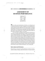
as the probability cutoff point while Table 3.9 shows the result taking 0.38
as the best probability cutoff point. The best cutoff point is determined by
examining the sensitivity and specifi city graph (Figure 3.4).
Table 3.9 shows that by using a probability cutoff of 0.50 and the low-income
poverty line in Data1, about 56 percent percent of the poor households are
correctly predicted (sensitivity), while 86 percent of nonpoor households
are accurately predicted by the model (specifi city). Positive predictive value
measures the percentage of correctly predicted poor households to the total
predicted poor households, while the negative predictive value measures
the ratio of correctly predicted nonpoor to the total predicted nonpoor. The

false positive rate for the true nonpoor indicates that 14 percent of nonpoor
households are inaccurately predicted as poor households, while the false
negative rate for the true poor indicates that 44 percent of poor households
are inaccurately predicted as nonpoor households. The false positive rate for
classifi ed poor shows that 33 percent of the total predicted poor households
are inaccurate, while 21 percent of the total predicted nonpoor households
are not correct as shown by the false negative rate for classifi ed nonpoor. The
Figure 3.4 Sensitivity and Specificity of the Logit Regression
Source: Authors’ calculation.
Data 1 (0.50 cut-off ) Data 2 (0.38 cut-off)
Table 3.9 Accuracy of Predicted Poverty Status by
Using Logit Regression and Low-Income Poverty Line
Probability Cutoff of 0.5
(Percent)
Probability Cutoff of 0.38
(Percent)
Data1 Data2 Data1 Data2
Sensitivity
55.59 55.73 72.09 72.61
Specificity
85.73 85.97 74.10 75.23
Positive predictive value
66.86 67.13 59.05 60.12
Negative predictive value
78.84 79.07 83.67 84.23
False positive rate for true nonpoor
14.27 14.03 25.90 24.77
False negative rate for true poor
44.41 44.27 27.91 27.39
False positive rate for classified poor

33.14 32.87 40.95 39.88
False negative rate for classified nonpoor
21.16 20.93 16.33 15.77
Correctly classified
75.44 75.70 73.41 74.34
Source: Authors’ calculation based on 2002 CRPMS.
Application of Tools to Identify the Poor
104 Identifying Poverty Predictors Using China’s Rural Poverty Monitoring Survey
overall accuracy of prediction is 75 percent. The general result for Data2 is
again close to Data1.
Using the probability cutoff point of 0.38, on the other hand, reveals that
the accuracy of poor household prediction is higher, that is, 72 percent, while
the accuracy of nonpoor household prediction is less, that is, 74 percent.
Meanwhile, the false prediction of the poor is less and the false prediction of
the nonpoor is higher. The overall accuracy of prediction is also a little bit
lower, that is 73 percent.
The stepwise procedure for the logit model is also implemented using the
offi cial absolute poverty line for Data1.
3
Table 3.10 reveals that, using the
offi cial absolute poverty line for defi ning the poverty status, only 17 percent
of the poor households are correctly predicted if the 0.50 probability cutoff
point was used. A simulation was also done using a different probability cutoff
(Table 3.10). The simulation showed that prediction accuracy can increase by
using a much lower probability cutoff point (0.16 in the simulation), but the
false rate for predicting poor also increases (to a high of almost 70 percent in
the simulation). The best cutoff point is determined by again examining the
sensitivity and specifi city graph in Figure 3.5. (See Appendix 3.6 for details.)
Summary and Conclusion
In the fi nal selection of the poverty predictors, all independent variables that

are signifi cant in both OLS and logistic models were chosen. (See Appendix
3.7.)
Both the multiple linear regression models and the logistic regression
model can accurately predict, by over 50 percent, which households are
3
The process was not conducted only for Data1 since the results of using Data 2 were
negligibly different, as shown in previous results (See details in Appendix 3.8.).
Table 3.10 Accuracy of Predicted Poverty Status by Using Logit
Regression and Official Absolute Poverty Line and Data 1
Probability Cutoff of 0.5 Probability Cutoff of 0.16
Sensitivity
17.41 73.17
Specificity
98.19 74.24
Positive predictive value
61.20 31.78
Negative predictive value
87.87 94.40
False positive rate for true non-poor
1.81 25.76
False negative rate for true poor
82.59 26.83
False positive rate for classified poor
38.80 68.22
False negative rate for classified non-poor
12.13 5.60
Correctly classified
86.80 74.09
Source: Authors’ calculation based on 2002 CRPMS.
Poverty Impact Analysis: Tools and Applications

Chapter 3 105
poor. The logistic regression model performs a little bit better than the OLS
regression model in terms of predicting the poverty status of the households.
Moreover, the logistic model is more fl exible for choosing a probability
cutoff point for higher prediction accuracy of the poor. The cost of doing
so, however, is an increase of false prediction, which will lead to a spillover
problem in program targeting. The modeling results show that predicting the
extremely poor is very diffi cult.
To determine the accuracy of logit models for predicting which households
are poor, the appropriate cutoff point is 0.38.
Figure 3.5 Sensitivity and Specificity of the Logit Regression
Using the Absolute Poverty Line for Data1
Source: Authors’ calculation.
Poverty Impact Analysis: Tools and Applications
Chapter 3 107
Appendix 3.1 Candidate Variables Selected
Variable Name Description
Welfare Indicators
consumpc Consumption expenditure per capita (yuan/person)
con_poor Is the household consumption expenditure below the poverty line? 1=yes, 0=no
inc_poor Is the household net income below the poverty line? 1=yes, 0=no
Household Head Characteristics
C4 Sex of the household head, 1=male, 0=female
C5 Age of the household head
spouse Whether the household head got married? 1=yes, 0=no
C7 Can household head speak Chinese? 1=yes, 0=no
C13 Education attainment of the household head
Household Demographics
Age0_14 Number of family members aged 0–14 years

Age15_60 Number of family members aged 15–60 years
Age60 Number of family members over 60 years old
studt Number of school age children in school
drops Number of school age children dropped out of school
C16 Are there any disabled adults at home? 1=yes, 0=no
laborr Ratio of labor to household members
B5 Family structure
Housing and Other Assets
B13 Whether has big animals? 1=yes, 0=no
B14 Whether has pigs? 1=yes, 0=no
B15 Whether has sheep or goats? 1=yes, 0=no
B16 Whether has poultry? 1=yes, 0=no
B17 Whether has a radio? 1=yes, 0=no
B18 Whether has a refrigerator? 1=yes, 0=no
B19 Whether has a TV? 1=yes, 0=no
B20 Whether has a bicycle? 1=yes, 0=no
B21 Whether has a motorcycle? 1=yes, 0=no
B22 Whether has a telephone? 1=yes, 0=no
B25 Whether has a car or truck? 1=yes, 0=no
B26 Whether has a hand tractor? 1=yes, 0=no
B27 Whether has a large-or medium-sized tractor? 1=yes, 0=no
B28 Whether has a cart? 1=yes, 0=no
B29 Whether has other agricultural tools? 1=yes, 0=no
B30 Whether has a draught animal? 1=yes, 0=no
B31 Whether has a production animal? 1=yes, 0=no
B34 Whether has a toilet? 1=yes, 0=no
B72 Is grain enough for consumption? 1=yes, 0=no
n_b73 Grain stored at home at the end of the year (kg/person)
n_b75 Grain stored for consumption at home at the end of the year (kg/person)
NB12 Whether the house is built with bricks or concrete? 1=yes, 0=no

n_b10 Square meters of living house per capita
B23 Square meters of production (business) house
B24 Square meters of barn for livestock
Natural Resources
landpc Cultivated land per capita, mu/per person
B45pc Forest land per capita (mu/person)
B46pc Orchard land per capita (mu/person)
B47pc Grassland areas per capita (mu/person)
B48pc Water areas under cultivation per capita (mu/person)
B49pc Wasteland areas per capita (mu/person)
B39 Whether is it difficult to access drinking water? 1=yes, 0=no
B41 Whether it become more difficult to collect fuels? 1=yes, 0=no
Activities and Access to Services
n_p Number of household members staying at home for 6 months or more
B3 Whether engaged in large-scale agricultural production? 1=yes, 0=no
leadbus Is any family members the village leader or engaged in business? 1=yes, 0=no
C21 Are there any household members who work outside? 1=yes, 0=no
cashr Ratio of sown areas of cash crop to total sown areas
fuel Whether use coal or gas for cooking? 1=yes, 0=no
B4 Whether a “wu bao hu” without any income sources, 1=yes, 0=no
B6 Whether participated in cooperatives? 1=yes, 0=no
B7 Whether participated in cooperative medical service? 1=yes, 0=no
B8 Whether has insurance? 1=yes, 0=no
C6 Does the household belong to ethnic minority groups? 1=yes, 0=no
B35 Whether has electricity? 1=yes, 0=no
bigevent Whether has a big event such as wedding, funeral, etc. 1=yes, 0=no
Community Characteristics
A1 Village physiognomy
A6 Number of natural villages with a road for motor vehicles
A14 Distance to the countryseat, km

A15 Distance to the town where the township government locates, km
A20 Distance to the nearby market, km
A50 Whether had a natural disaster in the village? 1=yes, 0=no
A57 Whether being designated as a poor village? 1=yes, 0=no
Source: Based on Household Survey Questionnaire.
Appendix
Application of Tools to Identify the Poor
108 Identifying Poverty Predictors Using China’s Rural Poverty Monitoring Survey
Appendix 3.2 Results of Stepwise Ordinary Least Square Regression Using Data1
(Dependent Variable: Log Per Capita Expenditure)
Variable Name Description Coefficient Standard Error P>|t|
Household Demographics
age0_14 Number of family members aged 0–14 years old 0.047 0.006 0.000
age15_60 Number of family members aged 15–60 years old 0.104 0.005 0.000
age60 Number of family members over 60 years old 0.095 0.007 0.000
studt Number of school age children in school 0.077 0.004 0.000
_Ib5_2 Households with a couple and one child 0.175 0.016 0.000
_Ib5_3 Households with a couple and two children 0.229 0.017 0.000
_Ib5_4 Households with a couple and three children or more 0.216 0.019 0.000
_Ib5_5 Households with father or mother and the children 0.206 0.025 0.000
_Ib5_6 Households with three generations 0.242 0.019 0.000
_Ib5_7 Other kinds of households 0.210 0.023 0.000
Household Head Characteristics
c4 Sex of the household head -0.066 0.017 0.000
c5 Age of the household head -0.001 0.000 0.001
spouse Whether the household head got married? 0.122 0.015 0.000
c7 Can household head speak Chinese? 0.089 0.019 0.000
_Ic13_2 Household head with primary school education 0.041 0.011 0.000
_Ic13_3 Household head with middle school education 0.084 0.012 0.000
_Ic13_4 Household head with high school education 0.112 0.014 0.000

_Ic13_5 Household head with technical secondary school education 0.181 0.029 0.000
_Ic13_6 Household head with college education and above 0.309 0.088 0.000
Housing and Other Assets
ro_n_b10 Square root of housing acreage 0.037 0.003 0.000
b23 Square meters of production (business) house 0.000 0.000 0.007
b24 Square meters of barn for livestock 0.001 0.000 0.001
b13 Whether has big animals? -0.045 0.011 0.000
b15 Whether has sheep or goats? -0.034 0.009 0.000
b17 Whether has a radio? 0.020 0.007 0.004
b18 Whether has a refrigerator? 0.075 0.015 0.000
b19 Whether has a TV? 0.094 0.008 0.000
b20 Whether has a bicycle? 0.022 0.007 0.004
b21 Whether has a motorcycle? 0.086 0.010 0.000
b22 Whether has a telephone? 0.146 0.009 0.000
b25 Whether has a truck? 0.093 0.032 0.004
b26 Whether has a hand tractor? 0.035 0.009 0.000
b30 Whether has a draught animal? 0.038 0.011 0.001
b31 Whether has a production animal? 0.036 0.008 0.000
b34 Whether has a toilet? 0.062 0.025 0.013
ro_n_b73 Square root of the amount of grain stored at home per capita 0.004 0.000 0.000
Natural Resources
b41 Whether it becomes more difficult to collect fuels? -0.030 0.007 0.000
landpc Cultivated land per capita 0.007 0.001 0.000
b45pc Forest land per capita 0.007 0.001 0.000
b47pc Grassland areas per capita 0.000 0.000 0.000
Activities and Access to Services
ln_p Log of family members staying at home for 6 months or more -0.936 0.017 0.000
b3 Whether engaged in large-scale agricultural production? 0.057 0.018 0.002
leadbus Is any family member the village leader or engaged in business? 0.089 0.011 0.000
c21 Any household members working outside? 0.088 0.008 0.000

cashr Ratio of sown areas of cash crop to total sown areas 0.139 0.017 0.000
fuel Whether use coal or gas for cooking? 0.032 0.007 0.000
b4 Whether a “wu bao hu” without any income sources -0.150 0.061 0.014
b7 Whether participated in cooperative medical service? -0.040 0.019 0.041
b8 Whether has insurance? 0.060 0.010 0.000
bigevent Whether has a big event? 0.195 0.008 0.000
Community Characteristics
_Ia1_2 Hilly areas 0.022 0.008 0.006
a6 Number of natural villages with a road for motor vehicles 0.002 0.001 0.022
a15 Distance to the town where the township government is located 0.001 0.000 0.033
a20 Distance to the nearby market 0.002 0.000 0.000
a50 Whether had a natural disaster in the village? -0.034 0.007 0.000
a57 Whether designated as a poor village? -0.047 0.006 0.000
Provincial Dummy
_Ipro_14 Shanxi -0.086 0.014 0.000
_Ipro_15 Inner Mongolia 0.103 0.017 0.000
_Ipro_22 Jilin -0.060 0.026 0.022
_Ipro_34 Anhui 0.177 0.017 0.000
_Ipro_36 Jiangxi 0.240 0.017 0.000
_Ipro_41 Henan 0.112 0.014 0.000
_Ipro_42 Hubei 0.288 0.016 0.000
_Ipro_43 Hunan 0.299 0.017 0.000
_Ipro_45 Guangxi 0.308 0.016 0.000
(continued on next page)
Poverty Impact Analysis: Tools and Applications
Chapter 3 109
Variable Name Description Coefficient Standard Error P>|t|
_Ipro_46 Hainan 0.284 0.037 0.000
_Ipro_50 Chongqing 0.271 0.019 0.000
_Ipro_52 Guizhou 0.223 0.014 0.000

_Ipro_53 Yunnan 0.155 0.013 0.000
_Ipro_63 Qinghai 0.340 0.025 0.000
_Ipro_64 Ningxia 0.144 0.026 0.000
_Ipro_65 Xinjiang 0.291 0.023 0.000
_cons 6.974 0.053 0.000
Number of obs = 22845
F( 72, 22772) = 273.58
Prob > F = 0.0000
Adj R-squared = 0.4621
P |t| = probability of accepting the null hypothesis (Ho)
Source: Authors’ calculation based on 2002 CRPMS.
Appendix 3.2 continued
Application of Tools to Identify the Poor
110 Identifying Poverty Predictors Using China’s Rural Poverty Monitoring Survey
Appendix 3.3 Results of Stepwise Ordinary Least Square Regression Using Data2
(Dependent Variable: Log Per Capita Expenditure)
Variable Name Description Coefficient Standard Error P>|t|
Household Demographics
age0_14 Number of family members aged 0–14 years old 0.032 0.006 0.000
age15_60 Number of family members aged 15–60 years old 0.096 0.005 0.000
age60 Number of family members over 60 years old 0.068 0.007 0.000
Studt Number of school age children in school 0.076 0.004 0.000
_Ib5_2 Households with a couple and one child 0.154 0.016 0.000
_Ib5_3 Households with a couple and two children 0.197 0.017 0.000
_Ib5_4 Households with a couple and three children or more 0.186 0.019 0.000
_Ib5_5 Households with father or mother and the children 0.143 0.025 0.000
_Ib5_6 Households with three generations 0.221 0.019 0.000
_Ib5_7 Other kinds of households 0.187 0.023 0.000
laborr Ratio of labor to household members -0.064 0.019 0.001
Household Head Characteristics

c4 Sex of the household head -0.045 0.017 0.008
c5 Age of the household head -0.001 0.000 0.011
spouse Whether the household head got married? 0.106 0.015 0.000
c7 Can household head speak Chinese? 0.075 0.021 0.000
_Ic13_2 Household head with primary school education 0.039 0.011 0.000
_Ic13_3 Household head with middle school education 0.086 0.011 0.000
_Ic13_4 Household head with high school education 0.114 0.014 0.000
_Ic13_5 Household head with technical secondary school education 0.216 0.028 0.000
_Ic13_6 Household head with college education and above 0.239 0.071 0.001
Housing and Other Assets
ro_n_b10 Square root of housing acreage 0.030 0.003 0.000
b23 Square meters of production (business) house 0.001 0.000 0.000
b13 Whether has big animals? -0.014 0.007 0.044
b14 Whether have pigs? 0.032 0.008 0.000
b17 Whether has a radio? 0.034 0.007 0.000
b18 Whether has a refrigerator? 0.039 0.014 0.006
b19 Whether has a TV? 0.103 0.008 0.000
b20 Whether has a bicycle? 0.037 0.007 0.000
b21 Whether has a motorcycle? 0.095 0.009 0.000
b22 Whether has a telephone? 0.123 0.008 0.000
b25 Whether has a truck? 0.133 0.032 0.000
b26 Whether has a walking tractor? 0.020 0.009 0.036
b28 Whether has a cart? -0.027 0.010 0.007
b29 Whether have other agricultural tools? 0.049 0.008 0.000
b31 Whether has a production animal? 0.033 0.008 0.000
b34 Whether has a toilet? 0.082 0.022 0.000
ro_n_b73 Square root of amount of grain stored at home per capita 0.004 0.000 0.000
Natural Resources
b39 Whether is it difficult to access drinking water? -0.018 0.008 0.019
landpc Cultivated land per capita 0.009 0.001 0.000

b45pc Forest land per capita 0.001 0.001 0.039
b46pc Orchard land per capita 0.020 0.006 0.001
b47pc Grassland areas per capita 0.001 0.000 0.000
Activities and Access to Services
ln_p Log of family members staying at home for 6 months or more -0.933 0.017 0.000
b3 Whether engaged in large-scale agricultural production? 0.104 0.018 0.000
leadbus Is any family members the village leaders or engaged in business? 0.087 0.010 0.000
c21 Any household members working outside? 0.091 0.007 0.000
cashr Ratio of sown areas of cash crop to total sown areas 0.104 0.017 0.000
b72 Is self-produced grain enough for consumption? 0.035 0.009 0.000
fuel Whether use coal or gas for cooking? 0.041 0.007 0.000
b4 Whether a “wu bao hu” without any income sources -0.175 0.060 0.003
b8 Whether has insurance? 0.061 0.010 0.000
bigevent Whether has a big event? 0.186 0.008 0.000
Community Characteristics
a6 Number of natural villages with road for motor vehicles 0.002 0.001 0.001
a20 Distance to the nearby market 0.002 0.000 0.000
a50 Whether had a natural disaster in the village? -0.035 0.006 0.000
a57 Whether designated as a poor village? -0.018 0.006 0.003
Provincial Dummy
_Ipro_14 Shanxi -0.034 0.015 0.021
_Ipro_15 Inner Mongolia 0.101 0.017 0.000
_Ipro_23 Heilongjiang 0.053 0.021 0.011
_Ipro_34 Anhui 0.223 0.017 0.000
_Ipro_36 Jiangxi 0.303 0.017 0.000
_Ipro_41 Henan 0.147 0.014 0.000
_Ipro_42 Hubei 0.388 0.016 0.000
_Ipro_43 Hunan 0.352 0.017 0.000
_Ipro_45 Guangxi 0.320 0.016 0.000
_Ipro_46 Hainan 0.289 0.037 0.000

(continued on next page)
Poverty Impact Analysis: Tools and Applications
Chapter 3 111
Variable Name Description Coefficient Standard Error P>|t|
_Ipro_50 Chongqing 0.278 0.019 0.000
_Ipro_52 Guizhou 0.237 0.014 0.000
_Ipro_53 Yunnan 0.175 0.013 0.000
_Ipro_63 Qinghai 0.311 0.025 0.000
_Ipro_64 Ningxia 0.088 0.026 0.001
_Ipro_65 Xinjiang 0.338 0.024 0.000
_cons 6.873 0.038 0.000
Number of obs = 23115
F( 72, 23042) = 282.63
Prob > F = 0.0000
Adj R-squared = 0.4673
Source: Authors’ calculation based on 2002 CRPMS.
Appendix 3.3 continued
Application of Tools to Identify the Poor
112 Identifying Poverty Predictors Using China’s Rural Poverty Monitoring Survey
Appendix 3.4 Results of Stepwise Logit Regression Using Data1
(Dependent Variable: Poor = 1, Nonpoor= 0)
Variable Name Description Coefficient Standard Error P>|z|
Household Demographics
age0_14 Number of family members aged 0–14 years old -0.173 0.038 0.000
age15_60 Number of family members aged 15–60 years old -0.377 0.032 0.000
age60 Number of family members over 60 years old -0.346 0.044 0.000
studt Number of school age children in school -0.320 0.023 0.000
_Ib5_2 Households with a couple and one child -0.762 0.096 0.000
_Ib5_3 Households with a couple and two children -1.052 0.101 0.000
_Ib5_4 Households with a couple and three childern or more -1.008 0.114 0.000

_Ib5_5 Households with father or mother and the children -0.859 0.149 0.000
_Ib5_6 Households with three generations -1.178 0.115 0.000
_Ib5_7 Other kinds of households -1.028 0.130 0.000
Household Head Characteristics
c5 Age of the household head 0.007 0.002 0.000
spouse Whether the household head got married? -0.363 0.080 0.000
c7 Can household head speak Chinese? -0.535 0.112 0.000
_Ic13_3 Household head with middle school education -0.179 0.038 0.000
_Ic13_4 Household head with high school education -0.338 0.063 0.000
_Ic13_5 Household head with technical secondary school education -0.332 0.166 0.045
_Ic13_6 Household head with college education and above -1.601 0.763 0.036
Housing and Other Assets
ro_n_b10 Square root of housing acreage -0.154 0.017 0.000
b23 Square meters of production (business) house -0.004 0.001 0.000
b15 Whether has sheep or goats? 0.220 0.050 0.000
b17 Whether has a radio? -0.109 0.038 0.005
b18 Whether has a refrigerator? -0.214 0.090 0.018
b19 Whether has a TV? -0.384 0.043 0.000
b21 Whether has a motorcycle? -0.391 0.058 0.000
b22 Whether has a telephone? -0.555 0.052 0.000
b26 Whether has a hand tractor? -0.107 0.052 0.040
b31 Whether has a production animal? -0.182 0.042 0.000
b35 Whether has electricity? -0.169 0.084 0.043
ro_n_b73 Square root of the amount of grain stored at home per capita -0.028 0.004 0.000
ro_n_b75
Square root of the amount of grain stored at home for
consumption per capita 0.009 0.004 0.047
Natural Resources
b39 Whether is it difficult to access drinking water? 0.122 0.043 0.005
b41 Whether it becomes more difficult to collect fuels? 0.107 0.037 0.004

landpc Cultivated land per capita -0.040 0.007 0.000
b45pc Forest land per capita -0.046 0.012 0.000
b47pc Grassland areas per capita -0.009 0.001 0.000
b49pc Wasteland areas per capita -0.091 0.022 0.000
Activities and Access to Services
ln_p Log of family members staying at home for 6 months or more 3.803 0.142 0.000
leadbus Is any family members the village leaders or engaged in business? -0.398 0.066 0.000
c21 Any household members working outside? -0.509 0.044 0.000
Cashr Ratio of sown areas of cash crop to total sown areas -0.616 0.099 0.000
b72 Is self-produced grain enough for consumption? 0.107 0.049 0.030
Fuel Whether use coal or gas for cooking? -0.226 0.041 0.000
b7 Whether participated in cooperative medical service? 0.239 0.103 0.020
b8 Whether has insurance? -0.239 0.060 0.000
bigevent Whether has a big event? -0.515 0.045 0.000
Community Characteristics
a6 Number of natural villages with a road for motor vehicles -0.011 0.004 0.008
a15 Distance to the town where the township government is located -0.007 0.002 0.002
a50 Whether had a natural disaster in the village? 0.196 0.037 0.000
a57 Whether designated as a poor village? 0.199 0.035 0.000
Provincial Dummy
_Ipro_14 Shanxi 0.348 0.077 0.000
_Ipro_15 Inner Mongolia -0.395 0.098 0.000
_Ipro_23 Heilongjiang -0.303 0.116 0.009
_Ipro_34 Anhui -0.730 0.100 0.000
_Ipro_36 Jiangxi -1.493 0.113 0.000
_Ipro_41 Henan -0.460 0.077 0.000
_Ipro_42 Hubei -1.351 0.102 0.000
_Ipro_43 Hunan -1.362 0.099 0.000
_Ipro_45 Guangxi -1.288 0.090 0.000
_Ipro_46 Hainan -1.344 0.194 0.000

_Ipro_50 Chongqing -1.277 0.116 0.000
_Ipro_52 Guizhou -0.984 0.073 0.000
_Ipro_53 Yunnan -0.558 0.066 0.000
_Ipro_63 Qinghai -1.199 0.142 0.000
_Ipro_64 Ningxia -0.468 0.143 0.001
_Ipro_65 Xinjiang -1.415 0.134 0.000
_cons -0.316 0.209 0.130
number of observations = 22845
number of groups = 10
Hosmer-Lemeshow chi2(8) = 7.61
Prob > chi2 = 0.4728
Source: Authors’ calculation based on 2002 CRPMS.
Poverty Impact Analysis: Tools and Applications
Chapter 3 113
Appendix 3.5 Results of Stepwise Logit Regression Using Data2
(Dependent Variable: Poor = 1; Nonpoor = 0)
Variable Name Description Coefficient Standard Error P>|z|
Household Demographics
age0_14 Number of family members aged 0–14 years old -0.090 0.038 0.018
age15_60 Number of family members aged 15–60 years old -0.309 0.032 0.000
age60 Number of family members over 60 years old -0.171 0.048 0.000
Studt Number of school age children in school -0.338 0.023 0.000
c16 Are there any disabled adults at home? -0.118 0.051 0.020
_Ib5_2 Households with a couple and one child -0.687 0.095 0.000
_Ib5_3 Households with a couple and two children -0.909 0.099 0.000
_Ib5_4 Households with a couple and three children or more -0.850 0.113 0.000
_Ib5_5 Households with father or mother and the children -0.619 0.144 0.000
_Ib5_6 Households with three generations -1.012 0.113 0.000
_Ib5_7 Other kinds of households -0.831 0.131 0.000
Household Head Characteristics

c4 Sex of the household head 0.198 0.099 0.046
c5 Age of the household head 0.004 0.002 0.037
Spouse Whether the household head got married? -0.354 0.083 0.000
_Ic13_2 Household head with primary school education -0.197 0.058 0.001
_Ic13_3 Household head with middle school education -0.422 0.062 0.000
_Ic13_4 Household head with high school education -0.535 0.079 0.000
_Ic13_5 Household head with technical secondary school education -0.829 0.183 0.000
Housing and Other Assets
ro_n_b10 Square root of housing acreage -0.118 0.017 0.000
b23 Square meters of production (business) house -0.004 0.001 0.000
b13 Whether has big animals? 0.078 0.039 0.047
b14 Whether have pigs? -0.203 0.044 0.000
b17 Whether has a radio? -0.152 0.038 0.000
b19 Whether has a TV? -0.471 0.042 0.000
b20 Whether has a bicycle? -0.191 0.043 0.000
b21 Whether has a motorcycle? -0.352 0.057 0.000
b22 Whether has a telephone? -0.553 0.051 0.000
b25 Whether has a truck? -0.461 0.194 0.018
b26 Whether has a hand tractor? -0.122 0.053 0.022
b28 Whether has a cart? 0.129 0.057 0.022
b29 Whether have other agricultural tools? -0.265 0.050 0.000
b31 Whether has a production animal? -0.157 0.043 0.000
b34 Whether has a toilet? -0.427 0.151 0.005
ro_n_b73 Square root of the amount of grain stored at home per capita -0.021 0.003 0.000
Natural Resources
landpc Cultivated land per capita -0.045 0.007 0.000
b45pc Forest land per capita -0.035 0.014 0.014
b46pc Orchard land per capita -0.292 0.075 0.000
b47pc Grassland areas per capita -0.005 0.001 0.000
Activities and Access to Services

ln_p Log of family members staying at home for 6 months or more 3.572 0.141 0.000
b3 Whether engaged in large-scale agricultural production? -0.303 0.105 0.004
leadbus
Is any family member the village leader or engaged in
business? -0.385 0.065 0.000
c21 Any household members working outside? -0.581 0.044 0.000
cashr Ratio of sown areas of cash crop to total sown areas -0.323 0.100 0.001
b72 Is self-produced grain enough for consumption? -0.124 0.049 0.011
fuel Whether use coal or gas for cooking? -0.197 0.041 0.000
b4 Whether a “wu bao hu” without any income sources 0.658 0.323 0.042
b8 Whether has insurance? -0.235 0.058 0.000
bigevent Whether has a big event? -0.540 0.046 0.000
Community Characteristics
_Ia1_3 Mountainous areas -0.098 0.044 0.025
a20 Distance to the nearby market -0.007 0.002 0.000
a50 Whether had a natural disaster in the village? 0.190 0.036 0.000
a57 Whether designated as a poor village? 0.076 0.035 0.028
Provincial Dummy
_Ipro_14 Shanxi 0.296 0.077 0.000
_Ipro_15 Inner Mongolia -0.495 0.099 0.000
_Ipro_23 Heilongjiang -0.425 0.116 0.000
_Ipro_34 Anhui -1.022 0.106 0.000
_Ipro_36 Jiangxi -1.574 0.112 0.000
_Ipro_41 Henan -0.528 0.081 0.000
_Ipro_42 Hubei -1.704 0.107 0.000
_Ipro_43 Hunan -1.747 0.103 0.000
_Ipro_45 Guangxi -1.148 0.090 0.000
_Ipro_46 Hainan -1.358 0.197 0.000
_Ipro_50 Chongqing -1.279 0.116 0.000
_Ipro_52 Guizhou -1.001 0.079 0.000

_Ipro_53 Yunnan -0.696 0.068 0.000
_Ipro_63 Qinghai -0.992 0.140 0.000
_Ipro_65 Xinjiang -1.130 0.093 0.000
_cons 0.131 0.218 0.548
Number of observations = 23115
Hosmer-Lemeshow chi2(8) = 12.58
Prob > chi2 = 0.1272
Source: Authors’ calculation based on 2002 CRPMS.
Application of Tools to Identify the Poor
114 Identifying Poverty Predictors Using China’s Rural Poverty Monitoring Survey
Appendix 3.6 Results of Stepwise Logit Regression Using the Absolute Poverty Line and
Dataset1 (Dependent Variable: Poor = 1, Nonpoor = 0)
Variable Name Description Coefficient Standard Error P>|z|
Household Demographics
age15_60 Number of family members aged 15–60 years old -0.238 0.027 0.000
age60 Number of family members over 60 years old -0.180 0.052 0.001
Studt Number of school age children in school -0.314 0.028 0.000
Drops Number of school age children dropped out of school 0.179 0.075 0.018
c16 Are there any disabled adults at home? 1=yes, 0=no -0.129 0.065 0.046
_Ib5_2 Households with a couple and one child -0.689 0.136 0.000
_Ib5_3 Households with a couple and two children -0.927 0.101 0.000
_Ib5_4 Households with a couple and three children or more -0.898 0.152 0.000
_Ib5_5 Households with father or mother and the children -0.790 0.120 0.000
_Ib5_6 Households with three generations -0.999 0.154 0.000
_Ib5_7 Other kinds of households -0.770 0.172 0.000
Household Head Characteristics
c5 Age of the household head 0.007 0.002 0.002
Spouse Whether the household head got married? -0.255 0.099 0.010
c7 Can household head speak Chinese? -0.347 0.127 0.006
_Ic13_3 Household head with middle school education -0.268 0.050 0.000

_Ic13_4 Household head with high school education -0.290 0.087 0.001
Housing and Other Assets
ro_n_b10 Square root of housing acreage -0.162 0.023 0.000
b24 Square meters of barn for livestock -0.008 0.001 0.00
b14 Whether have pigs? -0.125 0.056 0.026
b15 Whether has sheep or goats? 0.136 0.062 0.029
b19 Whether has a TV? -0.468 0.053 0.000
b21 Whether has a motorcycle? -0.362 0.080 0.000
b22 Whether has a telephone? -0.671 0.076 0.000
b26 Whether has a hand tractor? -0.198 0.070 0.005
b27 Whether has a large or medium sized tractor? 1=yes, 0=no 0.333 0.137 0.015
B28 Whether has a cart? 1=yes, 0=no 0.146 0.068 0.031
b35 Whether has electricity? -0.344 0.095 0.000
ro_n_b73 Square root of the amount of grain stored at home per capita -0.030 0.004 0.000
Natural Resources
b39 Whether is it difficult to access drinking water? 0.161 0.054 0.003
b41 Whether it becomes more difficult to collect fuels? 0.130 0.048 0.007
Landpc Cultivated land per capita -0.072 0.010 0.000
b45pc Forest land per capita -0.066 0.021 0.002
b47pc Grassland areas per capita -0.014 0.003 0.000
b49pc Wasteland areas per capita -0.160 0.043 0.000
Activities and Access to Services
ln_p Log of family members staying at home for 6 months or more 3.128 0.144 0.000
leadbus
Is any family members the village leaders or engaged in
business? -0.283 0.092 0.002
c21 Any household members working outside? -0.606 0.059 0.000
Cashr Ratio of sown areas of cash crop to total sown areas -0.505 0.129 0.000
b4
Whether a “wu bao hu” without any income sources,

1=yes, 0=no 0.942 0.363 0.010
bigevent Whether has a big event? -0.389 0.060 0.000
Community Characteristics
a20 Distance to the nearby market, km -0.009 0.002 0.000
a50 Whether had a natural disaster in the village? 0.245 0.049 0.000
a57 Whether designated as a poor village? 0.232 0.045 0.000
Provincial Dummy
_Ipro_14 Shanxi 0.205 0.092 0.026
_Ipro_15 Inner Mongolia -0.568 0.145 0.000
_Ipro_34 Anhui -1.191 0.161 0.000
_Ipro_36 Jiangxi -1.904 0.198 0.000
_Ipro_41 Henan -0.440 0.105 0.000
_Ipro_42 Hubei -1.586 0.167 0.000
_Ipro_43 Hunan -2.046 0.172 0.000
_Ipro_45 Guangxi -1.763 0.141 0.000
_Ipro_46 Hainan -1.739 0.292 0.000
_Ipro_50 Chongqing -1.785 0.207 0.000
_Ipro_52 Guizhou -1.497 0.111 0.000
_Ipro_53 Yunnan -0.699 0.095 0.001
_Ipro_62 Gansu -0.304 0.094 0.000
_Ipro_63 Qinghai -1.359 0.192 0.000
_Ipro_64 Ningxia -0.879 0.197 0.000
_Ipro_65 Xinjiang -1.629 0.167 0.000
_cons -0.727 0.296 0.014
number of observations = 22819
number of groups = 10
Hosmer-Lemeshow chi2(8) = 8.06
Prob > chi2 = 0.4275
Source: Authors’ calculation based on 2002 CRPMS.
Poverty Impact Analysis: Tools and Applications

Chapter 3 115
Appendix 3.7 Identified Poverty Predictors
Variable Name Description
Household Demographics
age0_14 Number of family members aged 0–14 years old
age15_60 Number of family members aged 15–60 years old
age60 Number of family members over 60 years old
studt Number of school age children in school
c16 Are there any disabled adults at home? 1=yes, 0=no
laborr Ratio of labor to household members
b5 Family structure
Household Head Characteristics
c4 Sex of the household head, 1=male, 0=female
c5 Age of the household head
spouse Whether the household head got married? 1=yes, 0=no
c7 Can household head speak Chinese? 1=yes, 0=no
c13 Education attainment of the household head
Housing and Other Assets
n_b10 Square meters of housing per capita
b23 Square meters of production (business) house
b24 Square meters of barn for livestock
b13 Whether has big animals? 1=yes, 0=no
b14 Whether has pigs? 1=yes, 0=no
b15 Whether has sheep or goat? 1=yes, 0=no
b17 Whether has a radio? 1=yes, 0=no
b18 Whether has a refrigerator? 1=yes, 0=no
b19 Whether has a TV? 1=yes, 0=no
b20 Whether has a bicycle? 1=yes, 0=no
b21 Whether has a motorcycle? 1=yes, 0=no
b22 Whether has a telephone? 1=yes, 0=no

b25 Whether has a car or truck? 1=yes, 0=no
b26 Whether has a hand tractor? 1=yes, 0=no
b28 Whether has a cart? 1=yes, 0=no
b29 Whether has other agricultural tools? 1=yes, 0=no
b30 Whether has a draught animal? 1=yes, 0=no
b31 Whether has a production animal? 1=yes, 0=no
b34 Whether has a toilet? 1=yes, 0=no
b35 Whether has electricity? 1=yes, 0=no
b72 Is grain enough for consumption? 1=yes, 0=no
n_b73 Grain stored at home at the end of the year (kg/person)
n_b75 Grain stored for consumption at home at the end of the year (kg/person)
Natural Resources
landpc Cultivated land per capita, mu/per person
b45pc Forest land per capita (mu/person)
b46pc Orchard land per capita (mu/person)
b47pc Grassland areas per capita (mu/person)
b49pc Wasteland areas per capita (mu/person)
b39 Whether is it difficult to access drinking water? 1=yes, 0=no
b41 Whether it becomes more difficult to collect fuels? 1=yes, 0=no
fuel Whether use coal or gas for cooking? 1=yes, 0=no
Activities and Access to Services
b3 Whether engaged in large scale agricultural production? 1=yes, 0=no
Leadbus Is any family members the village leaders or engaged in business? 1=yes, 0=no
n_p Number of household members staying at home for 6 months or more
c21 Are there any household members who work outside? 1=yes, 0=no
Cashr Ratio of sown areas of cash crop to total sown areas
b4 Whether a “wu bao hu” without any income sources, 1=yes, 0=no
b7 Whether participated in cooperative medical service? 1=yes, 0=no
b8 Whether has insurance? 1=yes, 0=no
bigevent Whether has a big event such as wedding, funeral, etc. 1=yes, 0=no

Community Characteristics
a1 Village physiognomy
a6 Number of natural villages with a road for motor vehicles
a15 Distance to the town where the township government is located, km
a20 Distance to the nearby market, km
a50 Whether had a natural disaster in the village? 1=yes, 0=no
a57 Whether being designated as a poor village? 1=yes, 0=no
pro Provincial code
Source: Authors’ calculation based on 2002 CRPMS.