Báo cáo toán học: "A note on packing chromatic number of the square lattice" ppsx

A note on packing chromatic number
of the square lattice
Roman Soukal
∗
Pˇremysl Holub
†
Submitted: Oct 27, 2009; Accepted: Mar 2, 2010; Published: Mar 15, 2010
Mathematics Subject Classification: 05C12, 05C15
Abstract
The concept of a packing colouring is related to a frequency assignment problem.
The packing chromatic number χ
p
(G) of a graph G is the smallest integer k such
that the vertex set V (G) can be partitioned into disjoint classes X
1
, . . . , X
k
, where
vertices in X
i
have pairwise distance greater than i. In this note we improve the
upper b ound on the packing chromatic number of the square lattice.
Keywords: Packing chromatic number, Packing colouring, Square lattice
1 Introduction
In this paper we consider only simple undirected graphs. We use [1] for terminology and
notation not defined here. Let dist
G
(x, y) denote the distance between vertices x and
y in G. The Cartesian product GH of graphs G and H is the graph with vertex set
V (G) × V (H), where vertices (x, y) and (x
′

, y
′
) are adjacent whenever xx
′
∈ E(G) and
y = y
′
, or x = x
′
and yy
′
∈ E(H). For two infinite paths P
1
, P
2
, the Cartesian product
P
1
P
2
is usually called the (infinite) square lattice.
The concept of the packing colouring comes from the area of frequency planning in
wireless networks, and was introduced by Goddard et al. in [3] under the name broadcast
colouring. The packing chromatic number of a graph G, denoted by χ
p
(G), is the smallest
integer k such t hat V (G) can be partitioned into k disjoint sets X
1
, . . . , X
k

, where f or
each pair of vertices x, y ∈ X
i
dist
G
(x, y) > i, for every i = 1, . . . , k. In other words,
vertices with the same colour i are pairwise at distance greater than i.
∗
Department of computer science and engineering, Univerzitni 22, 306 14 Pilsen, Czech Republic,
e-mail: Research supported by the Grant Agency of the Cz e ch Republic - the project
GA 201/09/0097.
†
Department of Mathematics, Univers ity of West Bohemia, and Institute for Theoretical Com-
puter Science (ITI), Charles University, Univerzitni 22, 306 14 Pilsen, Czech Republic, e-mail: hol-
Research Supported by Grant No. 1M0545 of the Czech Ministry of Education.
the electronic journal of combinatorics 17 (2010), #N17 1
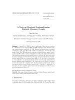
1 2 1 3 1 2 1 10 1 4 1 9 1 2 1 3 1 2 1 5 1 4 1 14
7 1 5 1 6 1 3 1 2 1 3 1 8 1 5 1 4 1 3 1 2 1 3 1
1 3 1 2 1 4 1 7 1 5 1 2 1 3 1 2 1 11 1 6 1 10 1 2
4 1 9 1 3 1 2 1 3 1 6 1 4 1 7 1 3 1 2 1 3 1 5 1
1 2 1 15 1 5 1 11 1 2 1 3 1 2 1 17 1 5 1 4 1 2 1 3
6 1 3 1 2 1 3 1 4 1 14 1 5 1 3 1 2 1 3 1 7 1 8 1
1 5 1 4 1 16 1 2 1 3 1 2 1 10 1 4 1 13 1 2 1 3 1 2
3 1 2 1 3 1 6 1 5 1 7 1 3 1 2 1 3 1 9 1 5 1 4 1
1 7 1 10 1 2 1 3 1 2 1 4 1 6 1 5 1 2 1 3 1 2 1 11
2 1 3 1 5 1 4 1 8 1 3 1 2 1 3 1 7 1 4 1 6 1 3 1
1 4 1 2 1 3 1 2 1 9 1 5 1 11 1 2 1 3 1 2 1 12 1 5
3 1 6 1 13 1 7 1 3 1 2 1 3 1 4 1 8 1 5 1 3 1 2 1
1 2 1 3 1 2 1 5 1 4 1 15 1 2 1 3 1 2 1 10 1 4 1 9
8 1 5 1 4 1 3 1 2 1 3 1 7 1 5 1 6 1 3 1 2 1 3 1

1 3 1 2 1 11 1 6 1 10 1 2 1 3 1 2 1 4 1 7 1 5 1 2
4 1 7 1 3 1 2 1 3 1 5 1 4 1 9 1 3 1 2 1 3 1 6 1
1 2 1 17 1 5 1 4 1 2 1 3 1 2 1 14 1 5 1 11 1 2 1 3
5 1 3 1 2 1 3 1 7 1 8 1 6 1 3 1 2 1 3 1 4 1 15 1
1 10 1 4 1 9 1 2 1 3 1 2 1 5 1 4 1 16 1 2 1 3 1 2
3 1 2 1 3 1 12 1 5 1 4 1 3 1 2 1 3 1 6 1 5 1 7 1
1 6 1 5 1 2 1 3 1 2 1 11 1 7 1 10 1 2 1 3 1 2 1 4
2 1 3 1 7 1 4 1 6 1 3 1 2 1 3 1 5 1 4 1 8 1 3 1
1 11 1 2 1 3 1 2 1 13 1 5 1 4 1 2 1 3 1 2 1 9 1 5
3 1 4 1 8 1 5 1 3 1 2 1 3 1 6 1 12 1 7 1 3 1 2 1
Figure 1: A pattern on 24 × 24 vertices.
Goddard et al. showed in [3] that the packing chromatic number of the infinite square
lattice is finite, more precisely between 9 and 23. Fiala a nd Lidick´y in [2] improved the
lower bound to 10, and Schwenk in [8] ha s shown t hat the packing chromatic number of
the infinite square lat tice is at most 22.
Using a computer we found the f ollowing result improving the upper bound of χ
p
(G)
for the infinite square lattice.
Theorem 1. Let G be the infinite square lattice. Then χ
p
(G)  17.
The square pattern on 24 × 24 vertices (see Figure 1) can be copied for the whole
infinite square lattice.
2 Method and algorithm
In [3] it was shown that to decide if, for a general graph G, χ
p
(G)  4 is NP-complete.
For this problem we used heuristics based on simulated annealing (SA).
SA is one method to determine a suboptimal solution of combinatorial problems,

the electronic journal of combinatorics 17 (2010), #N17 2
mostly NP-complete. This means that there is a large space of acceptable solutions
and it is not possible to find a globally optimal solution in polynomial time. As its name
implies, SA exploits an analogy between the way in which a metal cools and freezes into
a minimum energy crystalline structure (the a nnealing process) and the search for a min-
imum in a more general system. The algorithm is based upon that of Metropolis et al.
[6], which was originally proposed as a means of finding the equilibrium configuration of
a collection of atoms at a given temperature. The connection between this algorithm and
mathematical minimization was first noted by Pincus [7], but it was Kirkpatrick et al.
[4] who proposed that it for m the basis of an optimization technique for combinatorial
(and other) problems. SA’s maj or advantage over other methods is an ability to avoid
becoming trapped at local minima. The algorithm employs a random search which not
only accepts changes that decrease objective function f, but also some changes that in-
crease it. For more information about SA we refer to [5]. The main idea of SA algorithm
is that we iteratively search for a x
min
∈ D(f ) (where D(f ) is a definition scope of an
objective function f) such that f(x
min
) is as close as possible to the minimum of f(x).
The searching process is based on a degression of a temperature t. For a fixed t there
are several iterations and in each of these iterations we choose an arbitrary x
p
from a
neighbourhood of current x
min
(the radius of the neighbourhood depends on a current
iteration, higher iteration means smaller neighbourhood). A new x
p
is accepted with a

probability p = e
(f(x
min
)−f(x
p
))/t
which means, that a better solution (x
p
with smaller value
of f(x)) is accepted automatically (p  1) and a worse solution is accepted with a specific
probability, which decreases with lower temperature t.
3 Algorithms
In this section we present a pseudocode of used algor ithms. This varia tion of SA algorithm
gives us a colouring of a square pattern that we can repeat for the whole infinite square
lattice, and the obtained colouring is a packing colouring. Hence we can fill an infinite
square grid (each square on 24 × 2 4 vertices), where each square is represented by our
square pattern. The main idea is to colour as many vertices of a (partially filled) square
pattern with a current colour c as possible. We have a list of the best found patterns and
we memorize each pattern (up to symmetric patterns) with maximum number of vertices
coloured with c in this list. Thus we start with putting a colour one into an empty square
pattern, then we continue with putting a colour 2 into a pattern (patterns) filled with
colour one, etc., until at least one pattern from t he list of the best found patterns is whole
coloured.
In the pseudocode of Algorithm 1 we use two lists of patterns. The list Γ is a list of
the best found patterns (with the most number of coloured vertices) after colouring with
colour (c − 1). The list ∆ is a list of currently best found patterns after colouring with c.
We also define the following functions:
the electronic journal of combinatorics 17 (2010), #N17 3
(i) NonColoured (pattern K) - gives the number of non-coloured vertices in a pattern
K.

(ii) FreeForColour (colour c, pattern K) - gives the number of vertices of K which can
be coloured with a colour c. Note that if none of the vertices of K is coloured with c,
then FreeForColour (colour c, pattern K) = NonColoured (pattern K), and, on the
other hand, if there is a vertex in K coloured with c, then non-coloured vertices at
distance not greater than c cannot be coloured with c, hence FreeForColo ur ( colour
c, pattern K) < NonCo l oured (pattern K).
(iii) PlantColour (pattern K, colour c, temperature t) - puts current colour c in K under
a temperature t and returns a modified pattern L. Note that there is no vertex in
L which can be coloured with c.
For a current colour c and for each K ∈ Γ we use the function PlantCol our (pattern K,
colour c, temperature t) repeatedly, each time with a different temperature t (the value of
t is decreasing), and we memorize a new list of patterns ∆. The list ∆ contains patterns
in which we placed the current colour c the most times. If we find a new pattern in which
we used the colour c the same number of times as in patterns in ∆, we add this pattern
into ∆. If we find a new pattern in which we used the colour c more times than in patterns
in ∆, we clear the list ∆ and add this new pattern in it. This means that each patterns K
from the list ∆ has the same (and the smallest found) value of the function NonColoured
(pattern K).
The procedure for colouring of a pattern K with a current colour c is based on t he
following method, where we set a patt ern L as a copy of K. In k iterations, we are looking
for a vertex v which we colour with c. In each iteration we choose an arbitrary vertex
w of L, we get f(w) = FreeForColour (colour c, pattern L after colouring of w with c),
and we accept this vertex w (and set v = w) with a probability p = e
f (v)−f (w)
t
(see SA
algorithm), where f(v) = FreeForColour(c, L after colouring of v with c). Note that in
the first iteration we accept w automatically. After k iterations we colour the vertex v
with c and we repeat this method until FreeForColo ur (colour c, pattern L) = 0. When
FreeForColour (colour c, pattern L) = 0, we return L to Algo r ithm 1.

Remark
Let us note that we used this algorithm also for other shapes of pattern, e.g., rectangular
patterns on 16×24, 24×32 vertices and also a square pattern on 32×32 vertices. However,
the square pattern on 24 × 24 vertices gave the best solutions.
the electronic journal of combinatorics 17 (2010), #N17 4
Input: size of a pattern n
simulated annealing algorithm constants t
max
> t
min
> 0, q ∈ (0, 1)
Output: Γ - list of the best found patterns
// initialization step
Γ := empty list of the best found patterns;
pattern K := new pattern; // a null squared matrix of order n
add K to Γ;
colour c := 1; // c is a current colour
// end of the initialization step
// value of function nonColoured(K) is the same for all patterns K in Γ
// L is the first pattern in Γ
while nonColou red(L) > 0 do
∆ := empty list of patterns;
int p := nonColoured(L);
int m := 0; // m is a maximum number o f coloured vertices with current colour c
foreach K in Γ do
t := t
max
;
while t > t
min

do
T := pl antCo lour(K, c, t); // colour vertices o f K with c - see Algorithm 2
int a := p - nonColoured(T ); // a is number of vertices coloured with c in T
if a >= m then
// better possibility for colour c than patterns in ∆
if a > m then
∆ := empty list of patterns; // ∆ is cleared
m := a; // a is a new maximum number of vertices coloured with c
end
if T ∈ ∆ then
add T to ∆;
end
end
t := t ∗ q; // decrease temperature t
end
end
Γ := ∆; // put all the best found pa tt erns from ∆ to Γ
c := c + 1; // set a new colour c
end
return Γ; // return a list of the best found patterns
Algorithm 1: Main algo r ithm for determining a pattern of packing colouring of the
square latt ice
the electronic journal of combinatorics 17 (2010), #N17 5
Input: the original pattern K
the current colour c
the simulated annealing parameter t (temperature)
Auxiliary: the simulated annealing algorithm constant k (number of
iterations)
Output: pattern L - the original pattern K coloured with c
L := K; // L is a copy of K

// while there is at least one vertex in L which can be coloured with c
while f reeF o rColour(c, L) > 0 do
v := null; // v is a vertex colourable with c, at the beginning we have no such a
vertex
// f (v) is a number of vertices we lose for colouring with c while we colour v with c
// at the beginning f(v) is set as a maximum int value, because it will be minimized
int f(v) := max int value;
for i = 1 to k do
w := randomly chosen vertex from L which can be coloured with c;
// f (w) is a number of vertices we lose f or colouring with c while we colour w
with c
int f(w) := freeF orColour(c, L) − f reeF orColour(c, L with colou red w);
// SA accepts possibility with probability p = e
f (v)−f (w)
t
// if f (v) > f (w) then p > 1 and better possibility is accepted automatically
if random(0, 1) < e
f (v)−f (w)
t
then
f(v) := f(w);
v := w;
end
end
colour vertex v with c;
end
return L;
Algorithm 2: Function plantColou r(K, c, t)
the electronic journal of combinatorics 17 (2010), #N17 6
References

[1] J.A. Bondy, U.S.R. Murty, Graph Theory with Applications.
Macmillan, London and Elsevier (1976).
[2] J. Fiala, B. Lidick´y, Packing chromatic number for lattices.
Abstract in: Workshop Cycles and Colourings 2007 (I. Fabrici, M. Horˇn´ak, S. Jen-
drol’, eds.), IM Preprint, series A, No. 8/200 7.
[3] W. Goddard, S.M.Hedetniemi, S.T.Hedetniemi, J.M.Harris, D.F.Ra ll, Broadcast
chromatic numbers of Gra phs.
Ars Combin. 43 (1996), 149-157.
[4] S. Kirkpatrick, C.D. Gerlatt Jr., M.P. Vecchi, Optimization by Simulated Annealing.
Science 220 (1983), 671-680.
[5] P.J.M. van Laarhoven, E.H.L. Aarts, Simulated Annealing: Theory and Applications.
Reidel, Dordrecht, Holland (1987).
[6] N. Metropolis, A.W. Rosenbluth, M.N. R osenbluth, A.H. Teller, E. Teller, Equations
of State Calculations by Fast Computing Machines.
J. Chem. Phys. 21 ( 1953), 1087- 1092.
[7] M. Pincus, A Monte Carlo Method for the Approximate Solution of Certain Types
of Constrained Optimization Problems.
Oper. Res. 18 (1970), 1225-1228.
[8] A. Schwenk, personal communication, 2002.
the electronic journal of combinatorics 17 (2010), #N17 7