Báo cáo toán học: "Flexible Color Lists in Alon and Tarsi’s Theorem, and Time Scheduling with Unreliable Participants" pot
Bạn đang xem bản rút gọn của tài liệu. Xem và tải ngay bản đầy đủ của tài liệu tại đây (209.65 KB, 18 trang )
Flexible Color Lists in Alon and Tarsi’s Theorem,
and Time Scheduling with Unreliable Participants
Uwe Schauz
Department of Mathematics and Statistics
King Fahd University of Petroleum and Minerals
Dhahran 31261, Saudi Arabia
Submitted: Jul 21, 2008; Accepted: Dec 11, 2009; Published: Jan 5, 2010
Mathematics Subject Classifications: 91A43, 05C15, 05C20, 05C45
Abstract
We present a purely combinatorial proof of Alon and Tarsi’s Theorem about
list colorings and orientations of graphs. More precisely, we describe a winning
strategy for Mrs. Correct in the corresponding coloring game of Mr. Paint and Mrs.
Correct. This strategy produces correct vertex colorings, even if the colors are taken
from lists that ar e not completely fixed before the coloration process starts. The
resulting strengthening of Alon and Tarsi’s Theorem leads also to strengthening of
its numerous repercussions. For example we study upper bounds for list chr omatic
numbers of bipartite graphs and list chromatic in dices of complete graphs. As
real life application, we examine a ch ess tournament time scheduling problem with
unreliable participants.
Introduction
Alon and Tarsi’s Theorem [AlTa] f r om 1992, about list colorings and orientations of
graphs, has many applications in the theory of graph colorings. We will resume and
extend most of them in this article. However, Alon a nd Tarsi’s Theorem not only has
many applications, it also opened a door to a new very successful algebraic method. This,
so called Polynomial Method, was explicitly worked out in Alo n’s paper [Al2], where Alon
suggested the name Combinatorial Nullstellensatz fo r the main algebraic tool behind it.
We strengthened this Nullstellensatz in [Scha2] with a quantitative formula, and presented
some easy-to-apply corollaries and new applications. Our formula led in particular to a
quantitative version o f Alon and Tarsi’s Theorem [Scha2, Corollary 5.5].
the electronic journal of combinatorics 17 (2010), #R13 1
Apart from this very successful study of the algebraic method behind Alon and Tarsi’s
Theorem, combinatorialists always search for purely combinatorial proofs, since this usu-
ally helps to understand the situation in more detail. Indeed, Alon and Ta r si asked in their
original paper [AlTa] for such a proof. The first main purpose of this article is to present
one. Our proof actually gives some insight into the connection between orientations and
colorings, but also leads to a new strengthening. Even more, the work on this proof led
us to a new coloring game which provides an adequate game-theoretic approach to list
coloring problems and time scheduling problems with flexible lists of available time slots.
See [Al], [Tu] and [KTV] in order to get an overview of list colorings. We have already
presented this game of Mr. Paint and Mrs. Correct in [Scha3]. In this article we have
demonstrated that, even though the resulting notion of ℓ-paintability (Definition 1.2) is
stronger than ℓ-lis t colorability (ℓ-choosability), many deep theorems about list colorabil-
ity remain t r ue in the cont ext of paintability. In the present article we continue by giving
a combinatorial proof of a pa intability strengthening of Alon and Tarsi’s Theorem. After-
wards, we show that most applications of Alon and Tar si’s Theorem can be strengthened
as well.
In Section 1, we present a reformulated version of the game of Mr. Paint and Mrs.
Correct, and define ℓ-paintability as a strengthening of ℓ-list colorability.
In Section 2, we use this to give a purely combinatorial proof of a strengthening of
Alon and Tarsi’s Theorem (Theorem 2.1).
Section 3 is concerned with classical applications of Alon and Tarsi’s Theorem. We
use our strengthening to provide paintability versions of Alon and Tarsi’s bound of the
list chromatic numb er of bipartite and planar bipartite gr aphs (Theorem 3.3 and the
Corollaries 3.4 and 3.6). We even could refine their techniques, and improved their upper
bounds, in part icular with respect to the maximal degrees of t he vertices inside t he two
parties (as we call the partition parts) of the graph. Theorem 3.8 is anot her improvement
in this direction.
Furthermore, we present strengthened versions of Fleischner and Stiebitz’ Theo-
rem 3.9 about certain 4-regular Hamiltonian graphs, H
¨
aggkvist and Janssen’s bound
(Theorem 3.10) for the list chromatic index of the complete graph K
n
, and Elling-
ham a nd Goddyn’s confirmation of the list coloring conjecture for planar r-regular edge
r-colorable multigraphs (Theorem 3.12). Example 3.11 describes a time scheduling prob-
lem that demonstrates the advantage of the new painting concept against the list colo ring
approach with fixed list of available time slots.
We also mention, that in [HKS] we worked out a strengthening of Brooks’ Theorem,
based on our improved Alon-Tarsi-Theorem. Our result is even stronger than the version
by Borodin, Erd˝os, Rubin and Taylor. Its proof uses the existence of an induced even
cycle with at most one chord, and almost acyclic orientation.
the electronic journal of combinatorics 17 (2010), #R13 2
1 Mr. Paint and Mrs. Correct
In this short section we lay the g ame-theoretic foundation for the proof of Alon and Tarsi’s
Theorem. We introduced the game of Mr. Paint and Mrs. Correct in [Scha3]. It is a game
with complete information, played on a fixed given graph G = (V, E) . Here we use the G = (V, E)
following equivalent reformulation of the original game (which was first defined in [Scha3,
Game 1.6 & Definition 1.8]) :
Game 1.1 (Paint-Correct-Game). In this reformulation Mr. Paint has just one marke r.
Mrs. Correct has a fi nite stack S
v
of erasers for each vertex v in G
1
:= G . T hey are
lying on the corresponding vertices, ready for use.
The reformulated game of Mr. Paint and Mrs. Correct works as follows:
1P : Mr. Paint starts, choosing a nonempty set of ve rtices V
1P
⊆ V (G
1
) and marking
them with hi s mark e r.
1C: Mrs. Correct chooses an independent subset V
1C
⊆ V
1P
of marked vertices in G
1
,
i.e., uv /∈ E(G
1
) for all u, v ∈ V
1C
. She cuts off the vertices in V
1C
, so that the
graph G
2
:= G
1
\ V
1C
remains. The still ma rked vertices v ∈ V
1P
\ V
1C
of G
2
have
to be cleared. For ea c h such v ∈ V
1P
\ V
1C
Mrs. Correct has to use (and use up)
one eraser from the corresponding stack S
v
. She loses if she runs o ut of erasers
and cann ot do that, i.e., if already S
v
= ∅ for a still marked vertex v ∈ V
1P
\ V
1C
.
2P : Mr. Paint again chooses a no nempty set of vertices V
2P
⊆ V (G
2
) and marks them
with his marker.
2C: Mrs. Correct again cuts off an independen t set V
2C
⊆ V
2P
, so tha t a g raph G
3
:=
G
2
\ V
2C
remains. She also uses (and uses up) some erasers to clear the remaining
marked vertices v ∈ V
2P
\ V
2C
.
.
.
.
.
.
.
End: The game ends when one player canno t move anymore, and hence loses.
Mrs. Correct cannot move if she does not have enough erasers left to clear the
vertices she wa s not ab l e to cut off.
Mr. Paint loses if there are no more vertices left.
We may imagine that after each r ound the newly cut off vertices are colored with a
so far unused color. In this way a win for Mrs. Correct results in a proper coloring of the
underlying graph G . Whether this is possible or not possible depends on the sizes of the
stacks of erasers S
v
at the vertices v of G . We define:
the electronic journal of combinatorics 17 (2010), #R13 3
Definition 1.2 (Paintability). Let ℓ = (ℓ
v
)
v∈V
be defined by ℓ
v
:= |S
v
| + 1 . If there is ℓ, ℓ
v
a winning strategy for Mrs. Correct, then we say that G is ℓ-paintabl e .
We write n-“something” instead of (n1)-“something”, where 1 = (1)
v∈V
and n ∈ N . 1
It is not hard to see that ℓ-paintability is stronger (and in fact strictly stronger)
then ℓ-list colorability. The ℓ-paintability may be viewed as a dynamic version of list
colorability, where the color lists L
v
of sice ℓ
v
at the vertices v are not completely fixed
before the coloration process starts (see [Scha3] for details). We note down:
G is ℓ-paintable. =⇒ G is ℓ-list colorable. (1)
Many people ask if it really makes sense for Mr. Paint to choose in his i
th
move a
proper subset V
iP
⊂ V (G
i
) instead of taking the whole set V (G
i
) . Well, the point
is that Mrs. Correct may have a big or somehow advantageous independent set V
iC
in
V (G
i
) , and that Mr. Paint has to prevent her from cutting off this set by not marking
some vertices in it. The not marked and not cut off vertices may become the decisive
battlefield of the future. Sometimes patience succeeds. A partial attack V
iP
⊂ V (G
i
)
may cost less erasers, but can save vantage ground, ground that should be att acked only
if the surrounding vertices vertices already have lost more erasers. One example where
Paint’s winning strategy is like this is K
3,3
with one eraser at each vertex.
2 Alon and Tarsi’s Theorem
In this section we discus a surprising connection between colorings and orientations of
graphs. Let
G = (V, E, ) be an oriented graph, i.e., a graph G = (V, E) together with
G, e
an orientation : E ∋ e −→ e
∈ e . Suppose that we have a cartesian product →
L
L :=
v∈V
L
v
(2)
of lists L
v
of sizes ℓ
ℓ
v
:= |L
v
| > d
+
(v) , (3)
where d
+
(v) is the outdegree of v in
G . We view the elements λ ∈ L as vertex labellings, d
+
(v)
λ: v → λ
v
∈ L
v
, and ask: Is there a proper coloring λ ∈ L of G ?
One could co njecture that there is one, since each list L
v
(to each fixed vertex v ∈ V )
contains so many colors that – if all “successors” u of v ( vu in
G ) a r e already v→u
colored – ther e is at least one color in L
v
that differs from the colors of the successors
of v . If we now use this “evasion color” to color the vertex v , and do the same for all
other vertices of V , then we obtain a proper coloring of G , since in each edge uv one
end “takes care” of the other end (either vu or uv ).
However, this train of thought runs on nonexisting rails. We cannot just assume
that for each vertex v “all successors u of v are already colored”. An example which
the electronic journal of combinatorics 17 (2010), #R13 4
shows the validity of the desired conclusion is the directed cycle of length 3, which is not
colorable with 2 colors. Nevertheless, our consideration contains some plausibility, and
one could ask for an additional condition that makes it work. Alon and Tarsi found such
a condition in [AlTa]. They proved that ℓ-list colorings exist, if the sets of even and odd
Eulerian (spanning) subgraphs EE and EO of
G do not have the same size, i.e., EE, EO
|EE| = |EO| ; (4)
where a directed graph is even/odd Eulerian if it has even/odd many edges, and if the
indegree of each single ver tex v ∈ V equals its outdegree. In their paper they work
with the set D
α
= D
α
(G) = D
α
(
G) of all orientations ϕ with outdegree sequence D
α
, d
+
ϕ
d
+
ϕ
= (d
+
ϕ
(v))
v∈V
equal t o α ∈ Z
V
. They split this set into the sets DE
α
= DE
α
(
G)
D E
α
, DO
α
and D O
α
= DO
α
(
G) , of even resp. odd orientations ϕ ∈ D
α
, i.e., those which differ
from the fixed given reference orientation ( e
ϕ
= e
) on even resp. odd many edges
e ∈ E . At the end they used the fact that, with d
+
:= d
+
= (d
+
(v))
v∈V
, d
+
|DE
d
+
| = | EE| and |DO
d
+
| = | EO| . (5)
This is not hard to see (see also [Scha1, Lemma 2.6]). In this paper we state our theorems
using DE
α
and DO
α
instead of EO and EE . Of course,
DE
α
= DO
α
= ∅ (6)
if there are no ϕ ∈ D(G) with d
+
ϕ
= α , i.e., no real i zations of α . This is for example
the case if α
v
< 0 for o ne v ∈ V , or if
v∈V
α
v
= |E| , (7)
since
v∈V
d
+
ϕ
= |E| for all orientations ϕ ∈ D(G) . (8)
Alon and Tarsi’s work preceded the Combinatorial Nullstellensatz [Al2], which has
many applications. In [Scha2] we proved a quantitative strengthening of this Nullstel-
lensatz, which also led to a (weighted) qualitative version of the Alon-Tarsi Theorem.
The difference |DE
α
| − | DO
α
| (which can also be written as permanent of an incidence
matrix, as in [Scha2, Corrolary 5.5]) equals a weighted sum over certain colorings. Here,
we present a paintability strengthening of the result of Alon and Tarsi. Our proof can
be generalized to polynomials, as described in [Scha4], and leads to a pa intability version
of the Combinatorial Nullstellensatz. This version of the Nullstellensatz is more general
than the following strengthening of Alon and Tarsi’s Theorem. However, Alon and Tarsi
have a lready asked in the original paper [AlTa] for a combinatorial proof of their result.
Therefore, we work here in the purely combinatorial frame of orientations of graphs, in
order to shed some light on the surprising connection between colorings and orientations
of graphs. We have:
the electronic journal of combinatorics 17 (2010), #R13 5
Theorem 2.1. Let
G be a directed g raph and α ∈ N
V
, then
|DE
α
(
G)| = |DO
α
(
G)| =⇒
G is (α + 1)-paintable.
The proof of this theorem contains an explicit winning strategy. It is a proof by
induction, and uses the notations in Ga me 1.1. We will examine the orientatio n sets D E
α+N
U
D
S
:=
α
′
∈S
D
α
′
, DE
S
:=
α
′
∈S
DE
α
′
and DO
S
:=
α
′
∈S
DO
α
′
(9)
where ⊎ stands for disjoint union. Always S will be a set of the form ⊎
α + N
U
α + N
U
:= { α
′
α α
′
v
= α
v
for all v /∈ U } (10)
with α ∈ Z
V
and U ⊆ V ( α
′
α means α
′
v
α
v
for all v ∈ V ). Note that α does
not necessarily has to be a degree sequences, it plays a more general role here.
One single induction st ep in the aspirated proof will be partitioned into four parts. In
the first part we have to modify the induct io n hypothesis a little bit. The second part
describes the winning strategy of Mrs. Correct; it is mainly contained in the following
lemma. In the third part we have to understand why this strategy singles out an inde-
pendent set. This is also contained in the following lemma (in its very last sentence).
The final step is contained in the second lemma below, and will show that the induction
hypothesis remains true when we cut off the independent set. Figure 1 illustrates our
first lemma, in which we use the standard basis vectors 1
u
= (δ
u,v
)
v∈V
∈ {0, 1}
V
to the 1
u
indices u ∈ V with just o ne nonzero entry at v = u :
Lemma 2.2. Let
G = (V, E, ) be a directed graph, α ∈ N
V
, V
P
⊆ V nonempty and
u ∈ V
P
, then:
(i) (α − 1
u
) + N
V
P
= α + N
V
P
⊎ (α − 1
u
) + N
V
P
\u
.
(ii) DE
(α−1
u
)+N
V
P
= DE
α+N
V
P
⊎ DE
(α−1
u
)+N
V
P
\u and
DO
(α−1
u
)+N
V
P
= DO
α+N
V
P
⊎ DO
(α−1
u
)+N
V
P
\u
.
(iii) |DE
α+N
V
P
| = |DO
α+N
V
P
| implies that
|DE
(α−1
u
)+N
V
P
| = |DO
(α−1
u
)+N
V
P
| or
|DE
(α−1
u
)+N
V
P
\u
| = |DO
(α−1
u
)+N
V
P
\u
| .
(iv) |DE
α+N
V
P
| = |DO
α+N
V
P
| implies that there is a V
C
⊆ V
P
and an 0 α
′
α s.t.
|DE
α
′
+N
V
C
| = |DO
α
′
+N
V
C
| , α
′
|
V
C
≡ 0 and α
′
v
< α
v
for all v ∈ V
P
\ V
C
.
Each such set V
C
is independent in
G .
the electronic journal of combinatorics 17 (2010), #R13 6
Figure 1: v −→ α
v
and α + N
V
P
in Lemma 2.2.
or
α
N
6
5
4
3
2
1
0
V
V
P
v
6
v
5
v
4
v
3
v
2
v
1
.
.
.
.
.
.
.
.
.
.
.
.
or
α−1
v
3
N
6
5
4
3
2
1
0
V
V
P
\v
3
v
6
v
5
v
4
v
3
v
2
v
1
.
.
.
↓
.
.
.
.
.
.
or
α−1
v
3
N
6
5
4
3
2
1
0
V
V
P
v
6
v
5
v
4
v
3
v
2
v
1
.
.
.
.
.
.
.
.
.
.
.
.
· · ·
α
′
N
6
5
4
3
2
1
0
V
V
C
v
6
v
5
v
4
v
3
v
2
v
1
.
.
.
.
.
.
Proof. The elements σ of the set (α − 1
u
) + N
V
P
on the left side of Equation (i) fulfill
σ
u
α
u
− 1 . On the right side we simply distinguish between those with σ
u
> α
u
− 1
and those with σ
u
= α
u
− 1 .
In order to obtain part (ii), we just have to take the preimages of the sets in (i) under
the mapping ϕ −→ d
+
ϕ
, which we viewed either as a mapping defined on the set DE of D E
all even orientations, or as a mapping defined on the set DO o f all odd orientat io ns. D O
Now, we consider the cardinalities of the sets in part (ii) and o bta in
|DE
(α−1
u
)+N
V
P
| = |DE
α+N
V
P
| + |DE
(α−1
u
)+N
V
P
\u | and (11)
|DO
(α−1
u
)+N
V
P
| = |DO
α+N
V
P
| + |DO
(α−1
u
)+N
V
P
\u | . (12)
If we extend this system of linear equations with
|DE
(α−1
u
)+N
V
P
| = |DO
(α−1
u
)+N
V
P
| and (13)
|DE
(α−1
u
)+N
V
P
\u
| = |DO
(α−1
u
)+N
V
P
\u
| , (14)
it follows that
|DE
α+N
V
P
| = |DO
α+N
V
P
| . (15)
Part (iii) is t he contraposition to this conclusion.
In order to prove part (iv), we may use part (iii), as illustrated in Figure 1, to produce
sequences
α =: α
0
α
1
· · · α
t
0 and V
P
=: V
0
C
⊇ V
1
C
⊇ · · · ⊇ V
t
C
(16)
the electronic journal of combinatorics 17 (2010), #R13 7
with the property
|DE
α
i
+N
V
i
C
| = |D O
α
i
+N
V
i
C
| for i = 0, 1, . . . , t . (17)
Note that
α
t
|
V
t
C
≡ 0 (18)
if and only if the sequence of componentwise nonnegative α
i
in (16) can no longer be
extended through application of part (iii); hence, in this case par t (iv) holds, if we set
α
′
:= α
t
and V
C
:= V
t
C
. (19)
It remains to show that the existence of an edge uv with both ends in V
C
would lead to
a contradiction: Suppose there is one. Then turning this edge uv around gives rise to a
fixp oint free involution
Θ
uv
: D
N
V
(G)
∼
=
−−−−→ D
N
V
(G) . (20)
This involution can be restricted to an involution
D
α
′
+N
V
C
∼
=
−−−−→ D
α
′
+N
V
C
, (21)
since – if we apply Θ
uv
to an orientation ϕ ∈ D
α
′
+N
V
C
– the two changing outdegrees
d
+
ϕ
(u) and d
+
ϕ
(v) are irrelevant for its membership to D
α
′
+N
V
C
. That is because
α
′
u
= 0 and α
′
v
= 0 , (22)
by Equation (18), and because if σ := d
+
ϕ
belongs to α
′
+ N
V
C
then each σ
′
0 , which
differs from σ only on vertices w ∈ V
C
with α
′
w
= 0 , belongs to α
′
+ N
V
C
as well.
Altogether, as Θ
uv
maps even orientations to odd orientations and vice versa, we see
that
|DE
α
′
+N
V
C
| = |DO
α
′
+N
V
C
| , (23)
a contradiction.
Now we come to our second lemma which allows us t o cut off independent sets V
C
⊆ V .
For our main theorem we will need only the case V
P
= V
C
:
Lemma 2.3. Let
G = (V, E, ) be a directed graph, α ∈ N
V
, V
P
⊆ V , uv ∈ E , uv ,
E
′
⊆ E and le t V
C
⊆ V be an independent set in
G , then:
(i) |DE
α+N
V
P
(
G)| = |DE
(α−1
u
)+N
V
P
(
G\uv)| + |DO
(α−1
v
)+N
V
P
(
G\uv)| and
|DO
α+N
V
P
(
G)| = |DO
(α−1
u
)+N
V
P
(
G\uv)| + |DE
(α−1
v
)+N
V
P
(
G\uv)| .
(ii) |DE
α+N
V
P
(
G)| = |DO
α+N
V
P
(
G)| implies that
|DE
(α−1
u
)+N
V
P
(
G\uv)| = |DO
(α−1
u
)+N
V
P
(
G\uv)| or
|DE
(α−1
v
)+N
V
P
(
G\uv)| = |DO
(α−1
v
)+N
V
P
(
G\uv)| .
the electronic journal of combinatorics 17 (2010), #R13 8
(iii) |DE
α+N
V
P
(
G)| = |DO
α+N
V
P
(
G)| implies that there is an 0 α
′
α such that
|DE
α
′
+N
V
P
(
G \ E
′
)| = |DO
α
′
+N
V
P
(
G \ E
′
)| .
(iv) |DE
α+N
V
P
(
G)| = |DO
α+N
V
P
(
G)| implies that there is an 0 α
′′
α|
V \V
C
s.t.
|DE
α
′′
+N
V
P
\V
C
(
G \ V
C
)| = |DO
α
′′
+N
V
P
\V
C
(
G \ V
C
)| .
Proof. When we restrict an orientation ϕ of G to E\uv , we obtain an orientation of
the smaller graph G\uv . This restricted orienta tion ϕ|
E\uv
has the same parity (either
even or odd) as ϕ if u
ϕ
v , and the opposite parity in the other case. Conversely, each
orientation ϕ
′
of the smaller graph G\uv extends to one orientation of G with the same
parity as ϕ
′
, and to one orientat io n with the opposite orientation as ϕ
′
. The restriction
of the or ientations leads to bijections
DE
α+N
V
P
(
G)
∼
=
−−−−→ DE
(α−1
u
)+N
V
P
(
G\uv) ⊎ DO
(α−1
v
)+N
V
P
(
G\uv) and (24)
DO
α+N
V
P
(
G)
∼
=
−−−−→ DO
(α−1
u
)+N
V
P
(
G\uv) ⊎ DE
(α−1
v
)+N
V
P
(
G\uv) , (25)
and part (i) follows.
As in the proof of Lemma 2.2(iii), we deduce part (ii) from part (i). Likewise, iteration
of part (ii) yields part (iii), we just have to use that in inequalities of the form
|DE
α+N
V
P
(
G)| = |DO
α+N
V
P
(
G)| (26)
negative values of α may be replaced by zeros, as
DE
α
(
G) = ∅ = DO
α
(
G) for α 0 . (27)
In order to prove part (iv), at first, we remove the set E(U, W )
E
′
:= E(V
C
, V \V
C
) (28)
of all edges between V
C
and V \V
C
. Let 0 α
′
α be as in part (iii). As V
C
is independent, the vertices of V
C
are isolated in
G \ E
′
, so that, for all orientatio ns
ϕ: E \ E
′
→ V and all v ∈ V
C
,
d
+
ϕ
(v) = 0 (29)
and
d
+
ϕ
(v) ∈ α
′
v
+ N ⇐⇒ 0 = α
′
v
⇐⇒ d
+
ϕ
(v) = α
′
v
. (30)
It follows that
D
α
′
+N
V
P
(
G \ E
′
) = D
α
′
+N
V
P
\V
C
(
G \ E
′
) , (31)
and if we set
α
′′
:= α
′
|
V \V
C
, (32)
the electronic journal of combinatorics 17 (2010), #R13 9
this extends to
D
α
′
+N
V
P
(
G \ E
′
) = D
α
′
+N
V
P
\V
C
(
G \ E
′
) = D
α
′′
+N
V
P
\V
C
(
G \ V
C
) , (33)
where we have used that
E(
G \ E
′
) = E(
G \ V
C
) . (34)
Moreover, these equalities also hold when we replace D with DE or DO, so that the
inequality in part (iv) follows from those in part (iii).
With this we are prepar ed to describe the winning strategy required in the main proof:
Proof of Theorem 2.1. We present a winning strategy for Mrs. Correct, described in
the terms of Game 1.1. We suppose that, when the game has reached the i
th
round, Mrs.
Correct has (at least) α
i
v
erasers left at each vertex v of
G
i
, and that she has managed
to ensure
|DE
α
i
(
G
i
)| = |DO
α
i
(
G
i
)| , (35)
where α
i
= (α
i
v
)
v∈V (
G
i
)
∈ N
V (
G
i
)
. (For i = 1 ,
G
1
:=
G and α
1
:= α this holds.)
Now Mr. Paint makes his i
th
move:
iP: Mr. Paint chooses a nonempty subset V
iP
⊆ V (
G
i
) , and marks the vertices in V
iP
with his marker. If already V (
G
i
) = ∅ , then the game ends here, Mr. Paint is
defeated and Mrs. Correct wins.
Now, after Mr. Paint’s preselection, Mrs. Correct makes her i
th
move in the following
way, which is always possible, so that the game does not stop when it is her turn and she
indeed does not lose:
iC: Mrs. Correct knows from the induction hypothesis (35) that
D
α
i
(
G
i
) = ∅ , (36)
and, using double counting, she concludes that
v∈V (
G
i
)
α
i
v
= |E(
G
i
)| (37)
With the same reasoning she then sees, that
D
α
i
(
G
i
) = D
α
i
+N
V
iP
(
G
i
) (38)
so that the induction hypothesis (35) can be rewritten as
|DE
α
i
+N
V
iP
(
G
i
)| = |DO
α
i
+N
V
iP
(
G
i
)| . (39)
Now, she applies the algor ithm used in the proof of Lemma 2.2 (iv) to
G
i
, α
i
and
V
iP
in place of
G , α and V
P
, and obtains an independent set V
iC
:= V
C
and a
tuple α
′i
:= α
′
.
the electronic journal of combinatorics 17 (2010), #R13 10
Mrs. Correct knows from Lemma 2.2 (iv) that V
iC
is independent, and she cuts it
off. She further knows that for all still marked vertices v ∈ V
iP
\ V
iC
:
α
i
v
> α
′i
v
0 , (40)
so that there ar e enough erasers to clear the remaining markings. Moreover, at least
α
′i
v
erasers remain at each vertex v of
G
i
, and this will be enough to establish the
induction hypothesis for
G
i+1
:=
G
i
\ V
C
: (41)
As Mrs. Correct knows from Lemma 2.2 (iv),
|DE
α
′i
+N
V
iC
(
G
i
)| = |DO
α
′i
+N
V
iC
(
G
i
)| . (42)
Therefore, she can apply the algorithm behind Lemma 2.3 (iv) using the input
(
G, V
P
, V
C
, α) := (
G
i
, V
iC
, V
iC
, α
′i
) . She obtains a tuple α
i+1
:= α
′′
∈ N
V (
G
i+1
)
such that
|DE
α
i+1
(
G
i+1
)| = |DO
α
i+1
(
G
i+1
)| . (43)
This is exactly the induction hypothesis required for the next round, and since
α
i+1
v
α
′i
v
for all v ∈ V (
G
i+1
) , (44)
the values α
i+1
v
in this hypothesis are actually covered by t he numbers of erasers
in the remaining stacks S
v
.
The graph
G
i+1
and the reduced stacks S
v
of size ( at least) α
i+1
v
will be passed to the
next ro und. After some finite time t ∈ N , the g raph
G
t
will be empty, Mr. Paint cannot
move any more, and Mrs. Correct’s strategy succeeds.
3 Applications of Alon and Tarsi’s Theorem
There are several “classical” applications of Alon and Tar si’s Theorem. The proofs in
these applications lead to paintability statements, if we use our Theorem 2.1 instead of
the original version from Alon and Tarsi. In the first examples below, we also could
refine the originally used techniques, and obtain slightly better upper bounds and new
corollaries. These examples are based on the following definition, where, a s in this whole
section, we always assume that our graph G has edges, E(G) = ∅ :
L(G),
ˇ
L(G)
Definition 3.1.
L(G) := max
HG
|E(H)|
|V (H)|
and
ˇ
L(G) := max
HG
|E(H)|−1
|V (H)|
(1−
1
|E(G)|
)L(G) .
the electronic journal of combinatorics 17 (2010), #R13 11
This definition means that, if G is oriented, so that
|E(H)| =
v∈V (H)
d
+
H
(v) , (45)
then L(G) is simply the maximum value of the average outdegrees of the subgraphs
H = ∅ of G . Since average outdegrees are bounded by maximal outdegrees, this means
that we never will find an orientation ϕ: E −→ V of G with maximal outdegree ∆
+
(ϕ) ∆
+
(ϕ)
strictly smaller than L(G) , i.e.,
∆
+
(ϕ) L(G) (46)
for all orientations ϕ: E −→ V of G . However, the rounded up number ⌈L(G)⌉ L(G) ⌈ ⌉
is exa ctly the lowest possible maximal outdegree, as, e.g., shown in [AlTa, Lemma 3.1].
We extend this a little bit using the notation ⌊x⌋ x for rounded down numbers x ∈ R : ⌊ ⌋
Lemma 3.2. Any graph G = (V, E) has an orientation ϕ: E −→ V with
∆
+
(ϕ) = ⌈L(G)⌉ =
ˇ
L(G) + 1
.
Proof. Subdividing each edge e ∈ E with a new vertex ¯e yields a bipartite graph B
with vertex set
V (B) = V ⊎
¯
E . (47)
Replacing the original vertices v ∈ V ⊆ V (B) with
m :=
ˇ
L(G) + 1
>
ˇ
L(G) (48)
copies (v, 1) , (v, 2) , . . . , (v, m) of v we obtain a bipartite g r aph B
m
, where the inserted
vertices ¯e ∈
¯
E have degree 2m . Now, it is sufficient to find a matching of
¯
E in B
m
.
Such a matching ¯e −→ (v
¯e
, i
¯e
) would induce an orientation ¯ϕ: E −→ V of G via
e −→ ¯e −→ (v
¯e
, i
¯e
) −→ v
¯e
=: ¯ϕ(e) . (49)
Then the indegrees of ¯ϕ wold not exceed m , so that the opposite orientation ϕ would
fulfill
⌈L(G)⌉
(46)
∆
+
(ϕ) m =
ˇ
L(G) + 1
⌈L(G)⌉ , (50)
and the lemma would follow.
However, the existence of such a matching follows from Hall’s Theorem. We only have
to show that each nonempty vertex set
¯
F ⊆
¯
E has more than |
¯
F | − 1 neighbors in B
m
.
To this end, let F ⊆ E b e the set of edges in G corresp onding to
¯
F ⊆
¯
E . Let G[F ] G
be its induced subgraph, and let
F = V (G[F ]) ⊆ V be the set of all end-vertices of
edges in F . Then, indeed, the number of neighbors of
¯
F in B
m
is
m |
F | >
ˇ
L(G) |
F |
|E(G[F ])| − 1
|V (G[F ])|
|
F | = |
¯
F | − 1 . (51)
the electronic journal of combinatorics 17 (2010), #R13 12
Note that it can be advantag eous to use the second expression
ˇ
L(G) + 1
, instead
of ⌈L(G)⌉ , when one wants to utilize an upper bound for L(G) . We will see this below.
At first, we combine our results in the following theorem, similar to [AlTa, Theorem 3.4]:
Theorem 3.3. Bipartite graphs G are k-paintable for
k := ⌈L(G) + 1⌉ =
ˇ
L(G) + 2
.
Proof. Bipartite directed graphs
G do not contain odd Eulerian subgraphs, so that
|DO
d
+
(
G)|
(5)
= |EO(
G)| = 0 < |{∅}| |EE(
G)|
(5)
= |DE
d
+
(
G)| , (52)
and Theorem 2.1 applies. We just have to choose the orientation of
G in accordance
with Lemma 3.2.
As in [AlTa, Corollary 3.4] we obtain as corollary:
Corollary 3.4. Bipartite planar graphs are 3- paintabl e.
Proof. Every planar graph G is contained in a triang ulatio n with 3|V | − 6 edges, and
we have to remove at least one third of the edges (a t least one edge from each triangular
face) to obtain the original bipartite graph G . Hence, G contains at most 2|V | − 4
edges, and it follows that L(G) < 2 (since each subgraph H G is bipartite and planar
as well).
As it can be difficult to calculate L(G) or
ˇ
L(G) (1−
1
|E(G)|
)L(G) in Theorem 3.3,
we provide the following upper bounds:
Lemma 3.5. Let G = (V
1
⊎ V
2
, E) be a bi partite graph with parties V
1
and V
2
, and let
∆
i
(G) := max
v∈V
i
d(v) be the max i mal degree in side V
i
( i = 1, 2 ), then ∆
i
(G)
L(G)
1
1/∆
1
(G) + 1/∆
2
(G)
1
2
∆(G) .
Proof. Since E = ∅ , we may alow in the definition of L(G) , and in the minima below,
only subgraphs H with E(H) = ∅ , and can conclude:
1
L(G)
= min
HG
|V (H)|
|E(H)|
min
HG
|V (H) ∩ V
1
|
|E(H)|
+ min
HG
|V (H) ∩ V
2
|
|E(H)|
=
1
∆
1
(G)
+
1
∆
2
(G)
2
∆(G)
.
(53)
the electronic journal of combinatorics 17 (2010), #R13 13
With the “part ite” maximal degrees ∆
1
(G) , ∆
2
(G) from Lemma 3.5, we obtain the
following corollary to Theorem 3.3. Note that the upper bound in this corollary about
bipartite graphs is significantly better than those in Brooks’ Theorem (namely ∆(G) ) ,
even if we replace ∆
1
(G) and ∆
2
(G) with ∆(G) :
Corollary 3.6. Bipartite graphs G are
1 − 1/|E|
1/∆
1
(G) + 1/∆
2
(G)
+ 2
-paintable.
If we apply this cor ollary to K
2,3
\e (K
2,3
minus one edge), it tells us that this graph
is 2-paintable, which would not follow if we would have based our corollary only on the
expression ⌈L(G) + 1⌉ in Theorem 3.3. The small improvement
ˇ
L(G) (1−
1
|E(G)|
)L(G)
makes a difference, even though ⌈L(G) + 1⌉ =
ˇ
L(G) + 2
.
We want to go a little bit more into detail, and examine the possible orientations
in the bipartite case again. With the “partite” maximal degrees ∆
1
(G) , ∆
2
(G) from
Lemma 3.5 we obtain, in analogy to Lemma 3.2:
Lemma 3.7. Let G = (V
1
⊎ V
2
, E) be a bipartite graph with the two parties V
1
and V
2
.
For numbers L
1
, L
2
∈ N with
L
1
∆
1
(G)
+
L
2
∆
2
(G)
> 1−
1
|E|
holds:
There exists an orien tation ϕ: E −→ V
1
⊎ V
2
with d
+
ϕ
(v)
L
1
for all v ∈ V
1
,
L
2
for all v ∈ V
2
.
Proof. The proo f works exactly as those of Lemma 3.2. We just have to const r uct a
graph B
L
1
,L
2
with L
i
copies of the vertices in V
i
( i = 1, 2 ), instead of the graph B
m
.
Hall’s theorem is applicable in the modified proof, as each subset F ⊆ E of edges in G
“meets” at least |F |/∆
i
(G) vertices in V
i
, and this means that each subset
¯
F ⊆
¯
E of
new vertices has at least
L
1
|
¯
F |
∆
1
(G)
+
L
2
|
¯
F |
∆
2
(G)
> (1−
1
|E|
)|
¯
F | |
¯
F | − 1 (54)
neighbors in B
L
1
,L
2
.
It follows, exactly as in the more special case Theorem 3.3:
Theorem 3.8. Let G = (V
1
⊎ V
2
, E) be a bipartite graph with the parties V
1
and V
2
.
For numbers L
1
, L
2
∈ N with
L
1
∆
1
(G)
+
L
2
∆
2
(G)
> 1−
1
|E|
holds:
G is ℓ-paintable for ℓ = (ℓ
v
)
v∈V
1
⊎V
2
defined by ℓ
v
:=
L
1
+ 1 if v ∈ V
1
,
L
2
+ 1 if v ∈ V
2
.
If we apply this theorem to L
1
= L
2
:=
1−1/|E|
1/∆
1
(G) + 1/∆
2
(G)
+ 1
>
1−1/|E|
1/∆
1
(G) + 1/∆
2
(G)
, it
leads to the same upper bound as in Corollary 3.6.
the electronic journal of combinatorics 17 (2010), #R13 14
Fleischner and Stiebitz examined in [FlSt] 4-regular Hamiltonian graphs, and solved
a coloring problem of Erd˝o s (see also [Tu]). They made the following observation about
Eulerian subgraphs, which implies 3-paintability by Theorem 2.1 and (5):
Theorem 3.9. If a directed graph
G is the edge-disjoint union of a directed Hamiltonian
cycle and some mutually vertex-disj oint, cyclically oriented triangles, then
|EE(
G)| − |EO(
G)| ≡ 2 (mod 4) ,
and, consequently,
G is 3-paintable.
H
¨
aggkvist and Janssen found in [H
¨
aJa, Theorem 3.1] a bound for the list chromatic
index of the complete graph K
n
. This bound is best possible for odd n . Using The-
orem 2.1 instead of Alon and Tarsi’s classical version (which they use at the end of the
proof of [H
¨
aJa, Preposition 2.4]) we get:
Theorem 3.10. The complete graph K
n
is edge n-paintable.
Sketch of the proof. The line graph LK
n
of K
n
consists of n cliques Q
v
= K
n−1
, one
for each vertex v ∈ V (K
n
) . H
¨
aggkvist and Janssen extend each Q
v
to a K
n
by adding
a new vertex ¯v to it. Afterwards, they define a tuple α n − 1 such that the extended
line graph LK
n
has exactly one orientation ϕ with outdegree sequence d
+
ϕ
= α and with
no directed cycle inside one of the cliques Q
v
. Therefore, |D
α
(G)| is odd, the Alon-Tarsi
Condition in Theorem 2.1 applies, and the (α + 1)-paintability of LK
n
follows. Hence,
LK
n
is n-paintable and K
n
is edge n-paintable. H
¨
aggkvist and Janssen just use a
different notation and say α
¯v
is blocked out in Q
v
. In this way they come back to the
examination of orientations of the o r ig inal line gr aph LK
n
.
Based on this theorem we give an example that demonstrates the advantage of the
new painting concept against the list coloring approach:
Example 3.11 (Chess Tournaments). Five chess players are organizing a round robin
chess tournament. Each player shall play against each other exactly one time. In each
round at most ⌊
5
2
⌋ = 2 games can be played, as no player should play more then one
game at a time. Therefore, the
5
2
= 10 chess parties have to be played in at least 5
rounds, say on the five working days of a week. Indeed, K
¨
onig’s Theo r em tells us that
the chromatic index of K
5
is 5 so that 5 rounds are enough. Our five friends only have
to figure out how to do it in detail.
Now, H
¨
aggkvist and Janssen’s Theorem tells us that the list chromatic inde x of K
5
is 5 as well. What does this mean fo r our chess tournament? For example, it means that
the tournament can be scheduled in seven rounds/days, in such a way, that each player is
allowed to be unavailable on one day. Each player has to announce the day of his absence
in advance. If player A is not available on Sunday and player B does not have time
the electronic journal of combinatorics 17 (2010), #R13 15
on Wednesday, then still five days are left for their game to take place. In other words,
we have a list of at least five available time slots at each edge of K
5
, and H
¨
aggkvist and
Janssen’s Theorem guarantees that appropriate appointments can be made.
Now, our strengthening of H
¨
aggkvist and Janssen’s Theorem tells us that even the
paintability index of K
5
is 5 . In other words, Mrs. Correct has a winning strat egy in the
corresponding edge coloring game if there are 5 −1 = 4 erasers at each edge of K
5
(only
3 erasers per edge would not be enough). What do se this mean? Again, it means that
our tournament can be organized on seven days, in such a way, that each player is allowed
to miss one day. The new thing is that the players do not have to announce their absence
in advance. On each particular day of the tournament, it is the job of Mr. Paint to look
around and see who shows up. He then suggests that each present player should play
against all those other present players against whom he has not played so far. Since each
player should play only one party a t a time, his suggestion might be quite inapplicable,
and our smart Mr. Correct has to correct this proposal by selecting a matching inside
the suggested subgraph. Our Theorem 3.10 guarantees that she can do this in such a way
that after seven days all 10 games are played. This is because Mr. Paint will suggest
each edge of K
5
at least five times, if it is rejected again and again, and Mrs. Correct
can reject it at most four times.
This example can be generalized to tournaments of arbitrarily many players. However,
it could be that some days/rounds can be saved. For even n K
¨
onig’s Theorem states
that the chromatic index of K
n
is n − 1 , so that, e.g., another sixth player can join the
five-day tournament above, the
6
2
= 15 possible parties can be played on 5 days as
well. In other words, in the even case with always available players one day ca n be saved.
According to the List Coloring Conjecture, the list chromatic index of any graph equals
its chromatic index. Therefore, n − 1 should also be the list chromatic index of K
n
if n
is even, so that we should be able to save one day in the corresponding tournament with
disclosed days of absences. This would be best possible since the so-called total chromatic
number of K
2m
is ∆(K
2m
) + 2 = 2m + 1 , see [AlWi]. However, there seems to be no
published proof of the List Coloring Conjecture in the case of even complete gra phs.
Beyond this open problems, one could conjecture that the list colo ring index of a graph
equals it paintability index, which would extend the List Coloring Conjecture and would
apply to the third case in our example above. In this case n+1 rounds would be enough,
provided that n is even. If n 2 is odd, our bound o f n + 2 rounds is best possible.
That is because the n players may jointly attend the first n − 1 rounds. Afterwards,
there are two players, say A and B , who have not played against each other. Now, if
A does not show up in the n
th
round, and B does not show up in the (n+1)
th
round,
their game has to be staged in the remaining (n+2)
th
round.
A further generalization concerns the allowed number of absences. It seams that 2k
additional rounds are needed if k absences are allowed. Note also tha t our proof of
Theorem 3.10 and its repercussions is based on H
¨
aggkvist and Ja nssen’s proof and the
the electronic journal of combinatorics 17 (2010), #R13 16
proof of Theorem 2.1. This leads to a quite tricky strategy for Mrs. Correct, a n algorithm
with exponential running time. Brute force calculations might be as good.
We conclude this section with another special case of the List Coloring Conjecture.
Ellingham and Goddyn’s confirmed the List Coloring Conjecture for planar r-regular edge
r-colorable multigraphs G (see [ElGo] or the end of Section 5 in [Scha2]), and this can
be generalized to paintability. In their orig inal proof, they show that the difference
|DE
r−1
(
−−
LG)| − |DO
r−1
(
−−
LG)| , (55)
where
−−
LG is the arbitra rily oriented line graph of G , equals the number of edge
r-colorings of G (up to a constant factor). Thus, the existence of an edge r -coloring
implies the assumptions of Theorem 2.1, and hence the r-paintability of
−−
LG :
Theorem 3.12. Planar r-regular edge r-colorable multigraphs are edge r-paintable.
For arbitra r y graphs, the trick behind this theorem does not work. This is because the
corresponding difference of even and odd orientations usually equals just a weighted sum
over certain colorings [Scha2, Corollary 5.5(i)], so that the contributions of the different
colorings may cancel each other.
Acknowledgement:
We are grateful to Melanie Win Myint, Stefan Felsner, Anton Dochtermann, Caroline
Faria, Stephen Binns and Ayub Khan for helpful comments. Furthermore, the author
gratefully acknowledges the support provided by the King Fahd University of Petroleum
and Minerals, the Technical University of Berlin and the Eberhard Karls University of
T
¨
ubingen during this research.
References
[Al] N. Alon: Restricted Colorings of Graphs.
In “Surveys in combinatorics, 1993”, London Math. Soc. Lecture Notes Ser. 187,
Cambridge Univ. Press, Cambridge 1993, 1-33.
[Al2] N. Alon: Combinatorial Nullstellensatz.
Combin. Probab. Comput. 8, No. 1-2 (1999 ) , 7-29.
[AlTa] N. Alon, M. Tarsi: Colorings and Orientat io ns of Graphs.
Combinatorica 12 (1992), 125-134.
[AlWi] S. Alongkorn, C. Wichai: Behzad-Vizing Conjecture and Complete Graphs
CompleteGraphs.pdf
the electronic journal of combinatorics 17 (2010), #R13 17
[BKW] O. V. Borodin, A. V. Kostochka, D. R. Woodall:
List Edge and List Total Colourings of Multigraphs.
J. Comb i n. Theory Ser. B 71(2) (1997), 184-2 04.
[Di] R. Diestel: Graph Theory. (3rd edition) Springer, Berlin 2005.
[ElGo] M. N. Ellingham, L. Goddyn: List Edge Colourings of Some 1-Factorable Multi-
graphs. Combin atorica 16 (1996), 343-35 2.
[FlSt] H. Fleischner, M. Stiebitz: A Solution to a Colouring Problem of P. Erd˝os.
Discrete Mathematics 101 (1992), 39 -48.
[H
¨
aJa] R. H
¨
aggkvist, J. Janssen: New Bounds on the List-Chromatic Index of the Com-
plete Graph and Other Simple Graphs.
Combinatorics, Probability and Co mputing 6(3) (1997), 273–295.
[HKS] J. Hladk´y, D. Kr´al’, U. Schauz: Algebraic Proof of Brooks’ Theorem.
Submitted to Discrete Mathematics.
[JeTo] T. R. Jensen, B. Tof t: Graph Coloring Problems. Wiley, New York 1995.
[Minc] H. Minc: Permanents. Addison-Wesley, London 1978.
[KTV] J. Kratochv´ıl, Zs. Tuza, M. Voigt:
New Trends in the Theory of Graph Colorings: Choosability and List Coloring.
In: R.L. Graham et al . , Editors, Contemporary Tren ds in Discrete Mathematics.
DIMACS Ser. Di scr. Math. Theo. C omp. Sci. 49, Amer. Math. Soc. (1999) , 183–197.
[Scha1] U. Schauz: Colorings and Orientatio ns of Matrices and Graphs.
The Electronic Journal of Comb i natorics 13 (2006), #R61.
[Scha2] U. Schauz: Algebraically Solvable Problems:
Describing Polynomials as Equivalent to Explicit Solutions
The Electronic Journal of Comb i natorics 15 (2008), #R10.
[Scha3] U. Schauz: Mr. Paint and Mrs. Correct.
The Electronic Journal of Comb i natorics 16/1 (2009), #R77.
[Scha4] U. Schauz: A Paintability Version of the Combinatorial Nullstellensatz,
and List Colorings of k-partite k-uniform Hypergraphs.
In preparation.
[Tu] Zs. Tuza: Graph Colorings With Local Constraints – A Survey.
Discuss. Math. Graph Theory, 17, (1997), 161–228.
the electronic journal of combinatorics 17 (2010), #R13 18